A hydrodynamic slender-body theory for local rotation at zero Reynolds number
Abstract
Slender objects are commonplace in microscale flow problems, from soft deformable sensors to biological filaments such as flagella and cilia. Whilst much research has focussed on the local translational motion of these slender bodies, relatively little attention has been given to local rotation, even though it can be the dominant component of motion. In this study, we explore a classically motivated ansatz for the Stokes flow around a rotating slender body via superposed rotlet singularities, which leads us to pose an alternative ansatz that accounts for both translation and rotation. Through an asymptotic analysis that is supported by numerical examples, we determine the suitability of these flow ansatzes for capturing the fluid velocity at the surface of a slender body, assuming local axisymmetry of the object but allowing the cross-sectional radius to vary with arclength. In addition to formally justifying the presented slender-body ansatzes, this analysis reveals a markedly simple relation between the local angular velocity and the torque exerted on the body, which we term resistive torque theory. Though reminiscent of classical resistive force theories, this local relation is found to be algebraically accurate in the slender-body aspect ratio, even when translation is present, and is valid and required whenever local rotation contributes to the surface velocity at leading asymptotic order.
I Introduction
Capturing the fluid flow around a slender object at low Reynolds number has been a goal of countless research efforts, motivating the development of a range of theoretical approaches over the last seventy years. Perhaps best known amongst these is the resistive force theory introduced by Hancock [1], Gray and Hancock [2] in the 1950s, which established a simple, local approximation to the relationship between the velocity of a slender body and the force that it exerts on the surrounding fluid. Since these seminal works, resistive force theory has been iterated upon and refined into the broad class of slender-body theories, which exploit the asymptotic slenderness of an object to approximate and simplify the coupling between geometry and flow. This class of theories includes refinements to resistive force theory in complex environments [3, 4], as well as the integral equations of Wu and Yates [5], Johnson [6, 7], Keller and Rubinow [8], Higdon [9]. More recently, the emergence of regularised Green’s functions of Stokes flow [10] has prompted the development of regularised slender-body theories [11, 12, 13, 14], which are typically simpler to implement in practice than singular theories and can even afford additional flexibility [11, 12], though at the expense of a small regularisation error. Together, these slender-body theories have been utilised in the study of a wide range of biological and biophysical settings, such as in popular application to microscale motility and to the dynamics of synthetic sensors [15, 16, 12, 17, 18].
Broadly speaking, these slender-body theories seek to answer the following question: given a slender object that is translating in a fluid, what are the forces that are being exerted on the object as it moves relative to the fluid? This problem can be easily motivated by the aforementioned examples, with microscale swimming often involving significant side-to-side undulations of slender bodies, such as flagella or cilia, in order to achieve locomotion. Indeed, for slender objects that are not rapidly rotating, a statement that we will make precise in section II, the dominant contribution to the fluid flow at the surface of the body is from local translation, with the slenderness of the object reducing the magnitude of any rotational effects. However, if a slender object rotates sufficiently quickly, then local rotation can have a greater effect on the fluid than translation, which is readily seen to be the case for slender bodies that are not translating at all. Though the examples mentioned above are not often associated with rapid rotation, circumstances where rotation is significant arise in similar contexts. For instance, the twisting of slender bodies has been explored in detail in the context of filament instabilities, termed twirling and whirling in the study Wolgemuth et al. [19], motivated in part by the small-scale instabilities of DNA [20], though it is unclear if the scales associated with DNA are always compatible with the continuum fluid assumption. Further applications include ciliary beating [21] and exploring the shapes adopted by polymorphic bacterial flagella [22]. More recently, with the advent of efficient elastohydrodynamic simulation methods [23, 24], a need has arisen for accurate quantification of the hydrodynamic torques that act on slender bodies in flow. For instance, in a study of twisting and buckling, one can imagine imposing an arbitrarily large axial twist on an elastic filament in silico. The subsequent relaxation dynamics towards an untwisted equilibrium will then typically lead to rapid rotation of the slender body, with accurate study thereby warranting careful quantification of the fluid-imparted resistance to local rotation. Hence, the contribution of rotational motion cannot be neglected in general, motivating the development of a practical slender-body theory that is capable of accurately resolving rotational effects.
However, to the best of our knowledge and in spite of the significant attention given to translational theories, studies analysing, justifying and validating a rotational slender-body theory have been absent until a very recent study by Maxian and Donev [25]. However, the framework resulting from this initial study suffers from an undetermined parameter and, additionally, the restriction that the weighting of the Stokeslet in the single layer boundary integral formulation is equal to the surface traction, which necessarily assumes that the rotating body is constituted by a Newtonian fluid of the same viscosity as the surrounding medium. Such a restriction is inappropriate for cellular bioswimmers, for example due to the poroelasticity of eukaryotic cytoplasm [26].
Thus, as the primary aim of this study, we will seek to pose and present a detailed analysis of a slender-body theory that expressly accounts for rotational motion whilst imposing relatively weak restrictions, focussing in particular on regimes where angular velocity is sufficiently fast to contribute to the motion of the object at leading asymptotic order. In doing so, we will expand upon the rotation-capturing studies of Keller and Rubinow [8] and Koens and Lauga [27] by exploring a practical theory that we will demonstrate, both analytically and numerically, to be asymptotically accurate and broadly applicable.
Our initial slender-body ansatz, which we will introduce in LABEL:sec:rotating, will be strongly linked to the classical study of Chwang and Wu [28], which identified exact solutions for the flow around a range of axisymmetric bodies that were not necessarily slender. Here, we will look to relax this assumption of global axisymmetry, instead assuming slenderness and a notion of local axisymmetry, which we introduce formally later. Our analysis of this ansatz will motivate us to combine it with an existing, translational slender-body theory, which we will demonstrate is capable of capturing both the forces and torques acting on the body with asymptotic accuracy. Distinct in complexity from the general theory of Koens and Lauga [27], this combined ansatz will resemble those employed in an ad hoc manner in recent computational works [29, 30, 31, 32, 33], though here we will seek to formally justify its suitability and its accuracy, an assessment that we believe to be absent from previous studies. Thus, a further aim of this study will be to ascertain, to some degree, the suitability of a combined ansatz for the study of the general motion of locally axisymmetric slender bodies, incorporating both translation and rotation.
Hence, in this study, we will begin by precisely formulating the slender-body problem for locally axisymmetric objects in flow. Initially restricting ourselves to consideration of bodies that are undergoing local rotation only, without accompanying translation, we will asymptotically determine the suitability of this ansatz for accurately quantifying the torque exerted on the object by the fluid. Following further analysis of a simple numerical scheme suggested by this ansatz, we will move to consider motion that also includes translation, carefully justifying the coupling of our rotation-capturing ansatz with a traditional, translational slender-body theory. We will explore this theory asymptotically, culminating in a simple, local theory that is reminiscent of classical resistive force theories but with surprising asymptotic accuracy, and validate our theoretical results through numerical exploration.
II The rotating slender-body problem
II.1 Geometry and governing equations
Throughout, we will adopt the notation and set-up of Walker et al. [11], which we briefly summarise in dimensionless form and illustrate in LABEL:fig:setup. In this work, we will consider a three-dimensional, inextensible, unshearable slender body in a Newtonian fluid, with the fluid domain being taken to be the exterior of the slender body. In an inertial reference frame, the velocity of this fluid at a point is governed by the familiar dimensionless Stokes equations
| (1) |
where is the pressure. We will assume that the slender body is locally axisymmetric, such that its cross-section at any point is circular and lies in a plane transverse to the centreline [34]. With this assumption, the geometry of the body is entirely defined by its centreline and cross-sectional radius , where is a material arclength parameter. Here, is assumed to be non-negative, vanishing only at , in terms of which we can capture the slenderness of the body via
| (2) |
with slenderness defined as the regime , assumed throughout. This prompts the definition , so that is sharply bounded above by unity. In what follows, we will refer to this normalised function as the radius function.
The centreline and cross-sections of the body may be further described with the aid of the orthonormal triad , comprised of arclength-dependent unit tangent, normal, and binormal vectors to . More explicitly, these vectors satisfy the standard Frenet-Serret relations
| (3) |
with being the centreline curvature. This local basis allows us to define the radial unit vector , which lies in the transverse cross-section of the body, in terms of the cross-sectional angle as
| (4) |
with illustrated in figure 1b. With this notation, points on the surface of the slender body may be succinctly parameterised as
| (5) |
II.2 Boundary conditions
As is standard in slender-body applications, we will seek to apply the hydrodynamic no-slip condition on the surface of the slender body. For fluid velocity at a surface point parameterised by arclength and angle , we accordingly impose
| (6) |
where denotes dimensionless time. The velocity of the surface, which we will assume conserves the volume of the slender body, may be decomposed as
| (7) |
Here, is the linear or translational velocity and is the rate of local rotation about the centre of the cross section. Of note, this form includes, but is not limited to, rigid-body motion of the slender object. For completeness, the general no-slip condition may be stated as
| (8) |
III Rotating slender bodies
In this first exploration, we will adopt a simple, classically motivated ansatz and explore the efficacy of using it to satisfy the velocity boundary condition on slender bodies that are undergoing only rotation, i.e. .
III.1 A rotlet ansatz
Consider the following ansatz for the flow around a rotating slender body at a point :
| (9) |
where defines a notional eccentricity and the rotlet is given by
| (10) |
With these definitions, we have that is the torque density imparted on the fluid by the body, noting that we have non-dimensionalised the viscosity to unity, in line with Equation 9 of Chwang and Wu [35]. This rotlet is a fundamental singularity solution of Stokes equations, corresponding to the flow induced by point torque [36]. Hence, this ansatz represents the flow due to a line distribution of point torques, motivated by the classical study of Chwang and Wu [28], which employed a similar ansatz to study the rotation of axisymmetric bodies. Here, we have taken the limits of integration to be for later convenience, though note that they can readily be substituted for , representing only a minimal difference as as .
We will look to determine the suitability of this torque-only ansatz for satisfying a purely rotational boundary condition, so that we will impose
| (11) |
having set in equation 8. Of note, this boundary condition and ansatz, up to the limits of integration, are exactly of the form studied by Chwang and Wu [28] if we restrict our consideration to (1) straight slender bodies and (2) purely axial angular velocities, i.e. . Here, we will seek to retain generality in both the shape of the slender body and the considered angular velocity, with our assumptions of body slenderness and circular cross-sections in the transverse plane replacing Chwang and Wu’s assumption of axisymmetry.
III.2 Resistive torque theory
In order to evaluate the suitability of the ansatz of equation 9, we will pursue an asymptotic analysis in the slenderness parameter . Requiring that the ansatz of equation 9 satisfies the rotational boundary condition on the surface of the slender body yields the relation
| (12) |
which must hold for all and . If we denote the integrand by , we can make progress in evaluating the integral by noting that when 111That is, is both and not ., and when . Hence, the contributions of these regions to the integral are and , respectively. The difference in the size of the integrand between these two regions leads us to adopt the terminology of matched asymptotics, with defining the so-called inner region. In this case, asymptotic approximation of the rotlet integral is particularly straightforward, with only the inner region contributing to the integral at leading order in . In this region, we may expand in terms of an inner variable as
| (13) |
denoting this leading-order inner expansion by and making use of the local approximation . This expansion of is asymptotic if both and are , which each appear in terms that are . In terms of the integration variable , the leading-order inner expansion of equation 13 is
| (14) |
which decays like as moves away from the inner region. In particular, this inner expansion is only outside of the inner region, so that we can in fact write
| (15) |
with error scaling with , as the integral of outside the inner region is subleading. Thus, in order to evaluate the leading-order contribution of our ansatz, we need only evaluate the integral of . This integral decomposes into
| (16) |
where
| (17a) | ||||
| (17b) | ||||
For completeness, the required no-slip boundary condition reads
| (18) |
to leading order. Immediately, equation 18 presents cause for concern: the term containing is independent of , so represents a translational velocity generated by our ansatz, which is not compatible with the angular velocity boundary condition. However, for now, it is instructive to delay the consideration of this issue and proceed to try to relate to more simply.
In particular, we recall that the boundary condition must hold for all and , so that it must simultaneously hold for any given and at a fixed . Therefore, noting that from equation 4, we have the simultaneous equations
| (19a) | ||||
| (19b) | ||||
Notably, as the induced translational velocity is independent of , it is unaltered by this change in cross-sectional angle. Hence, this contribution cancels upon taking the difference between the two equations, yielding the relation
| (20) |
valid to leading order unless , which can only occur at the ends of the slender body. As is arbitrary in equation 20 and and are linearly independent, this equality between vector products allows us to conclude that
| (21) |
so that is proportional to with scale factor . This is a leading-order local relation between the rotation of a general slender body and the hydrodynamic torque that acts on it, which we term resistive torque theory (RTT).
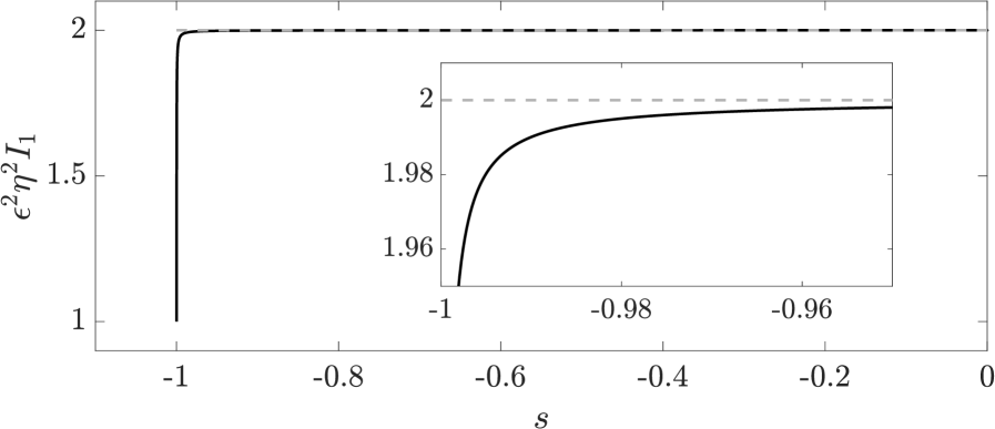
Further, we can explicitly evaluate as
| (22) |
This corresponds exactly to the result of Chwang and Wu [28, sec. 4] for straight, constant-torque bodies, highlighting that our leading-order asymptotic result is analogous to treating the slender body as locally straight with a constant torque density.
In our slender limit, we can further simplify the expression for . In particular, we note that we can write
| (23) |
For that are not too close to the ends of the body or, more precisely, those such that and , we can asymptotically expand and , yielding , so that
| (24) |
For approaching , we write for some such that
| (25) |
noting that by assumption. Here, we have , completely analogous to the case when was away from the ends of the body. However, expanding now yields
| (26) |
Hence, with , we have
| (27) |
as approaches , with an analogous result holding as approaches . The leading-order approximation to of equation 24 is illustrated in figure 2, highlighting excellent agreement with the exact expression of equation 22 away from the ends of the body. Hence, for the vast majority of the slender object, where equation 24 holds, we have the simple leading-order resistive torque theory relation
| (28) |
This resistive torque theory appears to hold for all components of and with the same coefficient of proportionality, in stark contrast to the anisotropic resistive force theory coefficients associated with the translation of slender objects in a viscous fluid. Further, if we were to restrict the rotation and the associated torque to be only in the axial direction, this is precisely in line with the relation found by Keller and Rubinow [8]. It is also useful to note that this result gives ready access to an analogue of a rotational drag coefficient for axial rotations of a straight slender body, with the relationship between an imposed, arclength-independent, axial rotation and the total torque on the body being readily accessible through integration of equation 28 in space. Explicitly, in terms of a total applied torque , we have the leading-order relation
| (29) |
recalling that we are in a dimensionless regime with dimensionless viscosity of unity.
III.3 Preventing unwanted translation
However, whilst the resistive torque theory of equation 28 is somewhat beguiling, we should no longer ignore the undesirable translational velocity associated with our rotlet ansatz, which we recall is generated by the product in equation 18. In order for our ansatz (and our derived resistive torque theory) to be suitable for satisfying the rotational boundary condition on our slender body, we need this term to vanish for each , so that we must have either or . However, we can directly evaluate as
| (30) |
which vanishes only at and generally scales as . Thus, to remove the unwanted translational velocities in general, it must be the case that whenever , so that the torque is almost-everywhere parallel to the local tangent . Recalling that our resistive torque theory of equation 28 states that is parallel to , this condition is equivalent (at leading order) to requiring that the rotation of the slender body is purely axial, so that is parallel to . Hence, the pure-rotlet ansatz examined in this section, and the resistive torque theory that it generates, is justified for use only for slender bodies that are locally rotating about their centreline.
III.4 Invertibility of the discretised rotlet ansatz
Given an angular velocity , an approach for determining the unknown torque density would be to discretise the centreline of the slender body into segments of length , approximating as being constant on each segment. Despite the simplicity of this approach, it is then unclear how best to apply the angular velocity boundary condition, as directly imposing the surface velocity at one randomly point on each of the segments can yield singular linear systems, which we reason arises due to the presence of the vector product in the integral kernel of LABEL:eq:_pure_rotletansatz. However, by following the reasoning that enabled us to invert equation 20, we can apply the boundary condition in a way that will provide sufficient information to solve for uniquely, subject to a condition on and .
In more detail, fixing an arclength on the th segment, we consider the three projections
| (31a) | ||||
| (31b) | ||||
| (31c) | ||||
of the full velocity boundary condition, which is being applied at the two points parameterised by and 222Our choice of here is for notational convenience only, with the argument readily modified to consider general .. The motivation behind our choice of these three projections becomes clear when considering the leading-order approximations to the rotlet integrals, which, following our expansion of equation 16, yields the leading-order form of LABEL:eq:_rotlet_bcprojection as
| (32a) | ||||
| (32b) | ||||
| (32c) | ||||
appealing to the cyclic property of the scalar triple product and the definition of from equation 4. In particular, it is clear that these local relations uniquely specify to leading order, so that the corresponding matrix representation is invertible. Hence, the block-diagonal linear system formed by imposing these leading-order relations for all would itself be invertible, constructed from invertible blocks. Strictly, this requires that be smaller than , so that the leading-order contributions of the rotlet integrals are associated with a single discrete .
This result does not immediately imply the invertibility of LABEL:eq:_rotletbc_projection, as the linear system formed from discretising the integrals of equation 31 would have non-zero off-diagonal blocks. However, fixing and assuming that , each of the off-diagonal blocks is strictly a factor of smaller than the diagonal block (in any suitable matrix norm), which follows from LABEL:eq:leading_order_expansion and the subsequent analysis. Hence, as there are such blocks, the total magnitude of the off-diagonal blocks scales with relative to the diagonal block, which we recall is invertible. Therefore, as this reasoning applies for each , the resulting linear system is block diagonally dominant, following the definition of Feingold and Varga [39], if . Thus, the block-matrix generalisation of the Gerschgorin circle theorem of Feingold and Varga [39] guarantees that the eigenvalues of the system are bounded away from zero, so that the system is invertible. Therefore, up to constants, we in fact have that the discretised rotlet ansazt, when implemented as described above, yields invertible linear systems if , establishing an approximate upper bound for for guaranteed invertibility.
IV Capturing translation
In the previous section, we saw that a flow ansatz comprised of only a distribution of rotlets was able to satisfy an angular-velocity boundary condition on the surface of a slender body, though the emergence of a torque-induced translational velocity limited the applicability of the ansatz to bodies that only rotate about their local tangent. In this section, we will seek to remove this restriction by augmenting the rotlet ansatz with a traditional slender-body theory ansatz that is capable of capturing translational motion.
However, the majority of slender-body theories are tailored to capturing translational surface velocities that preserve the volume of the slender body, invariably being a superposition of divergence-free singularities of Stokes flow. Indeed, these theories are only capable of representing volume-conserving flows [27]. Although the individual rotlet is volume-conserving, and hence so is the rotlet induced translational flow from the rotlet distribution of equation 9, this is not true for the general arclength-dependent imposed velocity field, in equation 8. Thus, we consider the constraints required for volume conservation, at least to , the level of asymptotic accuracy to which we will be working.
IV.1 Volume conservation
To proceed, we consider an arclength dependent velocity field and its associated net volume flux, defined by
| (33) |
where is as defined in equation 5, we have selected the outward-pointing surface normal, and we are integrating the volume flux over the entire surface of the slender body. In appendix A, we show that
| (34) |
with
Hence, if a translational velocity is imposed in equation 8, the constraints and ensure volume conservation to , with a correction at . In turn, these constraints require that the curvature is not too large, that the radius function does not vary too rapidly, and that the tangential velocity component is not too large. Finally, note that with once more and taking
| (35) |
so that and with , as confirmed a posteriori below via equation 50 and equation 51, we have and
| (36) |
This also provides an explicit self-consistency check that the asymptotic approximation to the translational flow velocity induced by the rotlet ansatz with the above curvature constraint also satisfies volume conservation to .
IV.2 A combined ansatz
As the induced translational velocity from the rotlet ansatz satisfies the condition of volume conservation to leading order in , we are able to account for it in our boundary condition via the addition of a translational slender-body theory. There are a wide range of candidate theories, including many of those touched upon in section I, though we will opt to use the recent theory of Walker et al. [11] as it both shares the notation used so far in this manuscript and generates volume-conserving translational surface velocities with algebraic asymptotic errors. Their translational ansatz is
| (37) |
whose limits of integration motivate our earlier choice of limits in LABEL:eq:pure_rotlet_ansatz. Here, is the force density applied to the fluid by the body, analogous to the torque density of the rotlet ansatz. The tensors and correspond to regularised Stokeslets and potential dipoles of Stokes flow [10], respectively, with a shared regularisation parameter . For completeness, these are of the form
| (38a) | ||||
| (38b) | ||||
where is the identity tensor. We refer the interested reader to the original publication of Walker et al. [11] for full details of their regularised slender-body theory. Here, we only note a key result of Walker et al.’s study: subject to and not varying too rapidly333The restriction on imposed by Walker et al. [11] was later refined by Walker and Gaffney [45], who noted that being Lipschitz continuous with an constant was sufficient., the leading-order flow that results from their ansatz at the surface of the slender body is independent of , so that it is purely translational. In symbols, this can be summarised as
| (39) |
for leading-order velocity , where the correction term depends on both and in general.
These properties, along with our analysis of the pure rotlet ansatz, motivate the following combined ansatz, suitable for a slender body with the general rigid-body velocity of equation 8:
| (40) |
Evaluated at the surface of the slender body and imposing the no-slip condition of equation 8, the boundary condition associated with this ansatz reads
| (41) |
with a typical slender-body problem then being to find the unknown force and torque densities given the translational and angular velocities. Owing to the established accuracy of the constituent translational and rotational ansatzes, the asymptotic accuracy of the combined ansatz is , so that the combined error relative to the surface velocity is .
IV.3 Enforcing no-slip in practice
If one were to seek to solve the integral equation of LABEL:eq:_combinedansatz_full_bc numerically, a quadrature rule might be employed to compute the integrals of the Stokeslet, potential dipole, and rotlet kernels. However, the combined ansatz and the associated integral equation can be significantly simplified using the results and principles of our analysis of the pure rotlet ansatz in section III, reducing the associated numerical cost. Specifically, we can bypass numerical evaluation of the rotlet integral entirely by applying the asymptotic result of section III, removing the need for quadrature for these integrals, though the integral involving the Stokeslet and potential dipole in equation 41 is always treated numerically in this study. In particular, retaining the leading-order rotlet terms, with relative errors of , yields
| (42) |
recalling that and are known in closed form from LABEL:eq:I1_exact and 30. With this approximate form, evaluating the contribution of the torque terms is akin to evaluating a resistive torque theory in terms of numerical cost.
A further theoretical simplification can be made by appropriately selecting the surface points at which to impose the no-slip condition. Inspired by our resistive torque theory result of section III, we are motivated to apply the boundary condition at the pairs of points and , with any -independent terms only needing to be computed once per pair. Imposing the condition of LABEL:eq:_partially_reducedconstraint at these points is equivalent to imposing LABEL:eq:_partiallyreduced_constraint at along with the modified constraint
| (43) |
at . This equivalence arises from noting that the latter condition is the result of taking the difference between equation 42 evaluated at both and . Equation 43 exploits the -independence of the imposed translational velocity and the rotlet-induced translation to eliminate these terms from the boundary condition, mimicking the reasoning employed in section III to generate our resistive torque theory.
IV.4 Generalised resistive torque theory
Equation 43 closely resembles an intermediate step in deriving the resistive torque theory of section III.2, akin to equation 20. The additional term in equation 43, , represents the effects of the sub-leading couple generated by the forces distributed along the body centreline, contributing to the angular velocity along with the local torque through equation 43. Hence, this equation captures the interactions between angular velocity, directly applied torques, and the sub-leading force-induced couple.
In pursuit of further simplification of this relation, we can estimate the magnitudes of the force- and torque-induced terms in equation 43. Recalling the expansion of equation 39 established by Walker et al. [11] for the translational slender-body theory ansatz, the force-induced terms scale as
| (44) |
though this is a crude upper bound as gross cancellation may occur between and . Furthermore, is bounded by both the prescribed velocity and the rotlet-induced translation, the latter being from equations 42 and 30, so that
| (45) |
The size of the rotlet-generated angular velocity in equation 43 is more simply estimated as
| (46) |
recalling that from equation 24. With these estimates, we can see that the direct angular velocity contribution of the rotlets in equation 43 algebraically dominates the angular velocity induced by the force density if
| (47) |
Should this condition hold, then we can neglect the term in equation 43 and incur relative errors. Indeed, if is smaller than the rotlet-induced translation, then this condition is satisfied without any additional constraints. Alternatively, if contributes to the dominant translational velocity, then our constraint becomes
| (48) |
Further, we can estimate the magnitude of by appealing to the calculations of Chwang and Wu [28], or equivalently to those of section III, to give the order-of-magnitude estimate , which agrees with simple scaling arguments. Hence, equation 48 becomes, after cancellation,
| (49) |
Thus, if the imposed translational velocity is at least a factor of smaller than the imposed angular velocity, we can neglect the force-induced angular velocity terms in equation 43 with relative errors.
In particular, we note that these conditions are satisfied precisely when the magnitude of is greater than or equal to that of . Hence, with reference to the no-slip condition of equation 8, the neglect of the force-induced angular velocity from LABEL:eq:_differenceboundary_condition is justified whenever the local rotation of the slender body is making a leading-order contribution to the overall no-slip condition, which is the focus and motivation of this study. In these circumstances, the angular velocity boundary condition of LABEL:eq:_difference_boundarycondition reduces to
| (50) |
with relative errors. Remarkably, this is precisely the relation of equation 20, valid whenever . Hence, following the reasoning of section III, we once again arrive at the resistive torque theory relation
| (51) |
Thus, the results of section III hold in more generality than we were originally able to conclude, valid for all and satisfying the above constraints. In particular, this resistive torque theory holds for all components of and , no longer limited to only axial angular velocities and torques. This validity extends to the asymptotic expansions of both near-to and far-from the endpoints of the slender body, so that, away from the ends of the body, we have the leading-order result
| (52) |
Noting that the torque density is given by , this slender-body result is fully consistent with the calculation of Koens and Lauga [27] for the torque density away from the end points of an axially rotating cylinder, which here we restrict to be slender. Again with a slenderness restriction, we also note that the above result is consistent with the calculation of the torque density for an axially rotating torus [41, 42].
V Numerical examples
In this section, we will present a number of numerical examples to support our asymptotic analysis. The numerical schemes used to explore these examples are standard, making use of non-specialised quadrature routines and direct linear solvers in MATLAB, with a comprehensive implementation available at https://gitlab.com/bjwalker/rotational-sbt. Throughout, as introduced in section III.4, we discretise the centreline of the slender body between and into equal intervals with midpoints , approximating unknown force and torque densities as constant on each segment. We will typically take in the computations that follow.
Having previously discussed the numerical implementation of the rotlet ansatz in section III.4, it remains to consider the discretised combined ansatz of section IV. In this case, with the discrete ansatz having vector unknowns, a natural choice would be to directly impose the velocity boundary condition at points on the surface, yielding a square linear system. However, when implementing this in practice, we invariably encountered linear systems with pathologically high condition numbers, typically on the order of , which posed a significant barrier to accurate numerical solution. Though we are not aware of the precise origin of this occurrence, we find that it may be successfully and simply circumvented by imposing manipulated boundary conditions, reducing the condition number to approximately . We achieve this by once again making use of the partial antisymmetry of the boundary condition on taking , with the details being presented in appendix B and following a similar principle to those detailed in section III.4 for the rotlet ansatz.
V.1 Axially rotating slender bodies
In order to evidence the ability of the pure rotlet ansatz of LABEL:sec:rotating to capture the axial rotation of slender bodies with various centrelines, we solve for the torque density in the rotlet ansatz as described in section III.4 for a range of slender bodies. The centrelines of the considered slender bodies are illustrated in LABEL:fig:_axially_rotatingbodies, with explicit parameterisations given in LABEL:app:_centrelineparams. We uniformly take , though the results that follow are not sensitive to this choice. In order to quantify the accuracy with which the rotlet ansatz satisfies the no-slip condition on the surface of the slender body, we define the absolute error measure
| (53) |
defining and to be the prescribed and numerically computed surface velocities at the point , respectively. This measure captures the greatest component-wise discrepancy between the numerical solution and the prescribed velocity on the surface, where the components are with respect to a fixed orthonormal laboratory basis.
For , a discrete approximation to this error is reported for both the full rotlet ansatz of LABEL:eq:_rotational_boundarycondition_ansatz, denoted by , and the resistive torque theory result of equation 28, denoted by . In both cases, the computed were inserted into equation 9, which was then evaluated at 612 distinct points on the surface of the body, at 51 discrete arclengths and 12 equispaced points around the circumference of each discrete cross section. In each of the cases reported, the rotlet ansatz can be seen to accurately capture the surface velocity of the slender body, with errors approximately on the order of , as predicted by the analysis of section III. The scaling of the error with is confirmed by comparing the errors for the two considered values of , denoted via subscripts as and , noting that in all cases except for the prolate spheroid in figure 3a. The error corresponding to the prolate spheroid is significantly lower than the other reported slender bodies, instead being limited by the accuracy of the employed quadrature and the discretisation of the slender body. We will return to consider the prolate spheroid, and the increased accuracy of the ansatz in this case, in section V.4. Remarkably, in all cases, the errors associated with the resistive torque theory result of LABEL:eq:rotating_rtt are of the same order as those associated with the full ansatz, including those slender bodies with curved centrelines, evidencing the validity of utilising the resistive torque theory in calculations involving axially rotating slender bodies.
| \begin{overpic}[width=73.7146pt]{axiallyRotatingBodies/A.eps}\put(0.0,90.0){(a)}\end{overpic} | \begin{overpic}[width=73.7146pt]{axiallyRotatingBodies/B.eps}\put(0.0,90.0){(b)}\end{overpic} | \begin{overpic}[width=73.7146pt]{axiallyRotatingBodies/C.eps}\put(0.0,90.0){(c)}\end{overpic} | \begin{overpic}[width=73.7146pt]{axiallyRotatingBodies/D.eps}\put(0.0,90.0){(d)}\end{overpic} | \begin{overpic}[width=73.7146pt]{axiallyRotatingBodies/F.eps}\put(0.0,90.0){(e)}\end{overpic} | |
V.2 Combining translation and rotation
Having established that the pure rotlet ansatz is capable of accurately satisfying velocity boundary conditions for axially rotating slender bodies, we now numerically explore its efficacy for capturing off-axis rotation of a prolate ellipsoid with , comparing its performance against the combined ansatz of section IV. Imposing the off-axis angular velocity and taking , we numerically solve for the forces and/or torques in the two ansatzes and evaluate the velocity at the surface evaluation points described in section V.1. The components of this velocity, including the prescribed boundary condition for comparison, are shown in figure 4, denoted , , and , respectively. As predicted by the analysis of section III, the rotlet ansatz is unable to capture the rotation without introducing additional, erroneous components of velocity on the order of in this case, whilst the combined ansatz successfully compensates for the rotlet-induced velocity and satisfies the boundary condition with .
V.3 Neglecting the force-induced couple
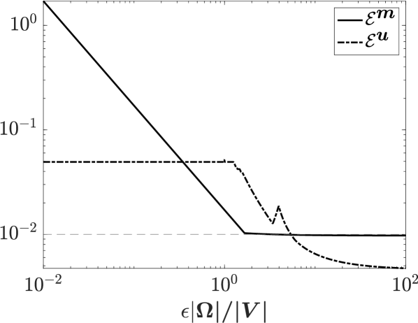
In section IV.4, we identified a regime in which the generalised resistive torque theory was accurate to leading order, which corresponded to cases where the angular velocity contributes to the velocity boundary condition at leading order. To numerically verify this conclusion, we consider a parabolic slender body, with centreline corresponding to figure 3b, taking and . For this slender body, we solve for the forces and torques on the body with , where are an orthonormal basis of the laboratory frame, and , varying the magnitude of . Here, we discretise the slender body into segments.
In figure 5, we show the maximum relative difference between the torques computed by the combined ansatz of LABEL:eq:_combinedansatz_full_bc and the resistive torque theory of section IV, treating the combined ansatz as the gold standard in the absence of an analytical solution. In symbols, this relative error measure is defined as
| (54) |
where and are the torques computed from the combined ansatz and from the resistive-torque-theory approximation to the combined ansatz, respectively. Note that, in the resistive torque theory solution, we directly compute the torques from the imposed angular velocity, then impose the full boundary condition of equation 41 at points on the surface of the body to yield the force density. Alongside this error, we show the analogous relative error in the velocity, defined as
| (55) |
where and are the velocities corresponding to the two ansatzes, respectively, generated by evaluating equation 40 with the computed forces and torques. These errors are shown as functions of the ratio between the magnitude of the angular velocity and the magnitude of the translational velocity, scaled by , with reference to the condition of LABEL:eq:_bound_on_V_andOmega. In particular, having taken in this example, the relative error in both the torque and velocity is on the order of for , as predicted by the asymptotic analysis of section IV.4.
V.4 Verification against an exact solution
Finally, as a limited yet informative analytical verification, we compare the computed forces and torques corresponding to the combined ansatz of section IV with the exact solution for the simultaneous rigid body translation and axial rotation of a prolate spheroid, as presented by Chwang and Wu [28, 35]. Specifically, we let and prescribe and . Chwang and Wu’s results yield the exact relations
| (56a) | ||||
| (56b) | ||||
which in fact hold for any constant translation and constant axial rotation . On writing this, we are setting , which gives rise to the parabolic torque profile of LABEL:eq:_CW_exact_soltorque. We compute the analogous numerical solutions for and from the full ansatz of equation 41, as described in appendix B, discretising the slender body using segments and taking . We observe componentwise errors on the order of in the forces and torques, limited by the numerical precision of the quadrature employed and the level of discretisation of the slender body. When employing the resistive torque theory of LABEL:eq:_generalrtt, these errors remain small but increase to approximately and for the force and torque, respectively, which further highlights the validity of the leading-order resistive-torque-theory approximation.
VI Discussion
In this study, we have posed and explored a simple rotlet ansatz for the flow around a locally rotating slender body, motivated by the classical solutions of Chwang and Wu [28] for axisymmetric bodies. In doing so, we have seen how such a rotlet ansatz is capable of capturing surface flows that result from locally axial rotations, whilst it can induce unwanted translational velocities if slender-body rotation is not purely axial. These induced flows were found to satisfy volume conservation to leading asymptotic order and, hence, we were able to make use of an established slender-body theory for translational motion to compensate for the linear velocities [11]. This resulted in a combined theory that is uniformly accurate to leading algebraic order in the aspect ratio of the slender body. Our combined ansatz is broadly applicable, being suited to bodies with circular cross sections and otherwise general shapes, including curved centrelines and spatially varying cross-sectional radii, subject to reasonable constraints on the centreline curvature and the arclength derivative of the radius function. Hence, we envisage its use in the future theoretical study of a range of slender bodies, in particular biological filaments such as cilia and flagella. Previous exploration into these application areas has made use of ansatzes similar to that developed here [31, 33, 32], though a detailed analysis of the suitability of the various ansatzes has been absent from previous works, to the best of our knowledge. Here, we have justified the validity of our posed ansatzes through a formal asymptotic analysis, ascertaining the capabilities and limitations of a pure rotlet ansatz and the flexibility afforded by a combined theory.
A notable consequence of our asymptotic analysis of the rotlet ansatz was the emergence of a local, leading-order relation between the angular velocity and torque, reminiscent of the formula provided by Chwang and Wu [28] for the torque on a rotating circular cylinder and the uniaxial result of Keller and Rubinow [8]. This so-called resistive torque theory, initially shown to be valid for axial rotations then extended to apply to general slender bodies (appropriately qualified in LABEL:sec:_generalisedresistive_torque_theory), arose with relative simplicity compared to the canonical resistive force theories developed since the mid 20th century [2, 1, 43]. The ready formulation of this theory was a consequence of the sharp near-singular nature of the rotlet kernel, which results in small region of the domain of integration being the algebraically dominant contribution to the rotlet ansatz. In contrast, the analogous Stokeslet integral kernel is less sharp, giving rise to the logarithmic errors typically associated with resistive force theories [7].
Owing to the algebraic errors and marked simplicity of the presented resistive torque theory, together with the absence of severe constraints, we anticipate that it will be of broad utility to slender body hydrodynamics. In particular, the combined theory of this study contains no restrictions preventing its application to chiral filaments, for instance, nor to the mobility problem, where velocities and angular velocities are determined given known force and torque densities. Furthermore, the presented framework provides an intuitive, leading-order link between angular velocity and torque that aligns with the classical results of Chwang and Wu [28], with simple ansatzae that are readily recognised as generalisations of this classical study. Finally, the present analysis also serves to justify the recent use of Chwang and Wu’s relation in the elastohydrodynamic method of Walker et al. [23], though Walker et al.’s work does not include non-local translational hydrodynamics.
When evaluating our slender-body ansatzes numerically in section V, we found that isolating the translational and angular velocities in turn significantly improved the condition number of the associated linear systems, which we achieved by taking various linear combinations of the boundary conditions. However, this result is purely empirical, with detailed analysis of this phenomenon warranting future consideration. In the case of the rotlet ansatz, we leveraged the same idea of taking particular linear combinations when forming our system of equations, which then enabled us to guarantee the invertibility of the system subject to the approximate bound . Though this condition is merely sufficient, not necessary, for invertibility, it suggests that the discretised ansatz may be unsuitable for numerical solution in this way if is larger than . This observation aligns qualitatively with anecdotal reports of instabilities identified in other slender-body theories, with often resulting in poor conditioning, or even numerical singularity, in practice. To the best of our knowledge, this issue remains both unreported and uninvestigated in the literature, with exploring the practical invertibility of the linear systems associated with discretised slender-body theories thereby representing a pertinent topic for future work, particularly given the popularity of slender-body theories. Another topic for future investigation is the accommodation of rotation in slender-body theories when the rotation is not sufficiently large for it to be within the leading-order kinematics, noting that recent advances in determining the higher order of slender-body theory by Koens [44], albeit possibly with a greater degree of non-locality.
In summary, we have explored the hydrodynamics of slender bodies in the Stokes regime, explicitly seeking to capture their local rotation via a slender-body ansatz for the fluid flow. Through the analysis of a classically inspired line distribution of rotlets, we have posed and validated a combined ansatz for capturing both translation and local rotation with errors that are uniformly algebraic in the slender body’s aspect ratio. Our asymptotic analysis also revealed a surprisingly simple local relation between the angular velocity and the torque on the body, leading to an algebraically accurate resistive torque theory that complements classical resistive force theories.
Acknowledgements
B.J.W. is supported by the UK Engineering and Physical Sciences Research Council (EPSRC), grant EP/N509711/1, and the Royal Commission for the Exhibition of 1851. K.I. acknowledges JSPS-KAKENHI for Young Researchers (Grant No. 18K13456), JSPS-KAKENHI for Transformative Research Areas (Grant No. 21H05309) and JST, PRESTO, Japan (Grant No. JPMJPR1921).
Appendix A Estimating the volume flux rate integral
For an arclength-dependent vector field we estimate the magnitude of the net volume flux rate integral
| (57) |
where is as defined in equation 5, the surface normal is outward and the integration is over the entire surface of the slender body. In order to evaluate the integral in equation 57, we compute the partial derivatives of with respect to and , yielding
| (58a) | ||||
| (58b) | ||||
where denotes and we define the azimuthal unit vector
| (59) |
which can equivalently be defined as . To arrive at equation 58a, we have made use of the additional Frenet-Serret relations
| (60) |
in which is the centreline curvature and is the accompanying torsion, the latter of which quantifies the non-planarity or intrinsic twist of the centreline. Equations 58a and 58b then lead to
| (61) |
noting that and . In particular, equation 61 captures the intuitive notion that the local surface normal is aligned approximately with , with corrections proportional to the rate of change of the cross-sectional radius with arclength.
Appendix B Numerical implementation of the combined ansatz
Having discretised the slender body into segments as described in section V, naively enforcing the velocity boundary condition of equation 41 at points on the surface of the slender body yields linear systems that, whilst empirically found to be invertible, typically have very high condition numbers, on the order of for and . However, we have found that enforcing alternative, mathematically equivalent conditions circumvents this problem, though we lack rigorous justification of this resolution. In detail, drawing inspiration from the invertible linear system constructed in LABEL:sec:invertibility and the approach of section IV.3, we impose six scalar boundary conditions at a fixed on the th segment. To do so succinctly, we note that the boundary condition of equation 41 can be written as
| (63) |
We further simplify this notation in this context by fixing , so that , , and depend only on , and retain only the explicit dependence of these terms, writing the boundary condition as
| (64) |
for brevity. With this compact notation, the first three scalar conditions that we impose involve taking the difference between the original boundary conditions evaluated at angles and , as we did in section IV.3, then projecting onto the local basis, as in section III.4. They read
| (65a) | ||||
| (65b) | ||||
| (65c) | ||||
analogous to those of equation 31 and implicitly evaluating and at . These conditions seek to capture only angular velocity contributions, with all -independent terms cancelling upon subtraction, as described in section IV.3. Notably, considering the leading-order terms in these boundary conditions leads to equations similar to that of equation 43, with the choice of components here guaranteeing invertibility of the rotlet contribution as in section III.4. We impose the three remaining scalar conditions by following a similar principle, but instead consider sums of the surface velocities, eliminating angular terms to isolate the effects of translation. These conditions can be summarised by the single vector condition
| (66) |
This overall approach can be viewed as attempting to decouple the translational and rotational flow problems. Empirically, we have found that this leads to linear systems of unproblematic condition number, typically on the order of for and , though establishing this analytically remains a topic for future study.
Appendix C Centreline parameterisations
References
- Hancock [1953] G. J. Hancock, The self-propulsion of microscopic organisms through liquids, Proceedings of the Royal Society of London. Series A. Mathematical and Physical Sciences 217, 96 (1953).
- Gray and Hancock [1955] J. Gray and G. J. Hancock, The Propulsion of Sea-Urchin Spermatozoa, Journal of Experimental Biology 32, 802 (1955).
- Brenner [1962] H. Brenner, Effect of finite boundaries on the Stokes resistance of an arbitrary particle, Journal of Fluid Mechanics 12, 35 (1962).
- Katz et al. [1975] D. F. Katz, J. R. Blake, and S. L. Paveri-Fontana, On the movement of slender bodies near plane boundaries at low Reynolds number, Journal of Fluid Mechanics 72, 529 (1975).
- Wu and Yates [1976] T. Y. Wu and G. Yates, Finite-amplitude unsteady slender-body flow theory, in 11th Symposium on Naval Hydrodynamics (1976).
- Johnson [1977] R. E. Johnson, Slender-body theory for Stokes flow and flagellar hydrodynamics, Ph.D. thesis, California Institute of Technology (1977).
- Johnson [1980] R. E. Johnson, An improved slender-body theory for Stokes flow, Journal of Fluid Mechanics 99, 411 (1980).
- Keller and Rubinow [1976] J. B. Keller and S. I. Rubinow, Slender-body theory for slow viscous flow, Journal of Fluid Mechanics 75, 705 (1976).
- Higdon [1979] J. J. L. Higdon, The hydrodynamics of flagellar propulsion: Helical waves, Journal of Fluid Mechanics 94, 331 (1979).
- Cortez [2001] R. Cortez, The method of regularized Stokeslets, SIAM Journal on Scientific Computing 23, 1204 (2001).
- Walker et al. [2020a] B. J. Walker, M. P. Curtis, K. Ishimoto, and E. A. Gaffney, A regularised slender-body theory of non-uniform filaments, Journal of Fluid Mechanics 899, A3 (2020a).
- Gillies et al. [2009] E. A. Gillies, R. M. Cannon, R. B. Green, and A. A. Pacey, Hydrodynamic propulsion of human sperm, Journal of Fluid Mechanics 625, 445 (2009).
- Cortez and Nicholas [2012] R. Cortez and M. Nicholas, Slender body theory for Stokes flows with regularized forces, Communications in Applied Mathematics and Computational Science 7, 33 (2012).
- Olson et al. [2013] S. D. Olson, S. Lim, and R. Cortez, Modeling the dynamics of an elastic rod with intrinsic curvature and twist using a regularized Stokes formulation, Journal of Computational Physics 238, 169 (2013).
- Guglielmini et al. [2012] L. Guglielmini, A. Kushwaha, E. S. G. Shaqfeh, and H. A. Stone, Buckling transitions of an elastic filament in a viscous stagnation point flow, Physics of Fluids 24, 123601 (2012).
- Smith et al. [2009] D. J. Smith, E. A. Gaffney, J. R. Blake, and J. C. Kirkman-Brown, Human sperm accumulation near surfaces: a simulation study, Journal of Fluid Mechanics 621, 289 (2009).
- Roper et al. [2006] M. Roper, R. Dreyfus, J. Baudry, M. Fermigier, J. Bibette, and H. A. Stone, On the dynamics of magnetically driven elastic filaments, Journal of Fluid Mechanics 554, 167 (2006).
- Olson and Fauci [2015] S. D. Olson and L. J. Fauci, Hydrodynamic interactions of sheets vs filaments: Synchronization, attraction, and alignment, Physics of Fluids 27, 121901 (2015).
- Wolgemuth et al. [2000] C. W. Wolgemuth, T. R. Powers, and R. E. Goldstein, Twirling and Whirling: Viscous Dynamics of Rotating Elastic Filaments, Physical Review Letters 84, 1623 (2000).
- Liu and Wang [1987] L. F. Liu and J. C. Wang, Supercoiling of the DNA template during transcription., Proceedings of the National Academy of Sciences 84, 7024 (1987).
- Holwill et al. [1979] M. E. Holwill, H. J. Cohen, and P. Satir, A Sliding Microtubule Model Incorporating Axonemal Twist and Compatible with Three-dimensional Ciliary Bending, Journal of Experimental Biology 78, 265 (1979).
- Macnab and Ornston [1977] R. M. Macnab and M. K. Ornston, Normal-to-curly flagellar transitions and their role in bacterial tumbling. Stabilization of an alternative quaternary structure by mechanical force, Journal of Molecular Biology 112, 1 (1977).
- Walker et al. [2020b] B. J. Walker, K. Ishimoto, and E. A. Gaffney, Efficient simulation of filament elastohydrodynamics in three dimensions, Physical Review Fluids 5, 123103 (2020b).
- Schoeller et al. [2020] S. F. Schoeller, A. K. Townsend, T. A. Westwood, and E. E. Keaveny, Methods for suspensions of passive and active filaments, Journal of Computational Physics , 109846 (2020).
- Maxian and Donev [2022] O. Maxian and A. Donev, Slender body theories for rotating filaments, Journal of Fluid Mechanics 952, A5 (2022).
- Moeendarbary et al. [2013] E. Moeendarbary, L. Valon, M. Fritzsche, A. R. Harris, D. A. Moulding, A. J. Thrasher, E. Stride, L. Mahadevan, and G. T. Charras, The cytoplasm of living cells behaves as a poroelastic material, Nature Materials 12, 253 (2013).
- Koens and Lauga [2018] L. Koens and E. Lauga, The boundary integral formulation of Stokes flows includes slender-body theory, Journal of Fluid Mechanics 850, R1 (2018).
- Chwang and Wu [1974] A. Chwang and T. Y.-T. Wu, Hydromechanics of low-Reynolds-number flow. Part 1. Rotation of axisymmetric prolate bodies, Journal of Fluid Mechanics 63, 607 (1974).
- Flores et al. [2005] H. Flores, E. Lobaton, S. Mendezdiez, S. Tlupova, and R. Cortez, A study of bacterial flagellar bundling, Bulletin of Mathematical Biology 67, 137 (2005).
- Nazockdast et al. [2017] E. Nazockdast, A. Rahimian, D. Zorin, and M. Shelley, A fast platform for simulating semi-flexible fiber suspensions applied to cell mechanics, Journal of Computational Physics 329, 173 (2017).
- Ishimoto and Gaffney [2018] K. Ishimoto and E. A. Gaffney, An elastohydrodynamical simulation study of filament and spermatozoan swimming driven by internal couples, IMA Journal of Applied Mathematics 83, 655 (2018).
- Huang et al. [2019] J. Huang, L. Carichino, and S. D. Olson, Hydrodynamic interactions of actuated elastic filaments near a planar wall with applications to sperm motility, Journal of Coupled Systems and Multiscale Dynamics 6, 163 (2019).
- Carichino and Olson [2019] L. Carichino and S. D. Olson, Emergent three-dimensional sperm motility: coupling calcium dynamics and preferred curvature in a Kirchhoff rod model, Mathematical medicine and biology : a journal of the IMA 36, 439 (2019).
- Antman [2005] S. S. Antman, Nonlinear Problems of Elasticity, Applied Mathematical Sciences, Vol. 107 (Springer-Verlag, New York, 2005).
- Chwang and Wu [1975] A. T. Chwang and T. Y.-T. Wu, Hydromechanics of low-Reynolds-number flow. Part 2. Singularity method for Stokes flows, Journal of Fluid Mechanics 67, 787 (1975).
- Kim and Karrila [1991] S. Kim and S. J. Karrila, Microhydrodynamics, Butterworth - Heinemann series in chemical engineering (Elsevier, 1991).
- Note [1] That is, is both and not .
- Note [2] Our choice of here is for notational convenience only, with the argument readily modified to consider general .
- Feingold and Varga [1962] D. G. Feingold and R. S. Varga, Block diagonally dominant matrices and generalizations of the gerschgorin circle theorem, Pacific Journal of Mathematics 12, 1241 (1962).
- Note [3] The restriction on imposed by Walker et al. [11] was later refined by Walker and Gaffney [45], who noted that being Lipschitz continuous with an constant was sufficient.
- Chwang and Hwang [1990] A. T. Chwang and W. Hwang, Rotation of a torus, Physics of Fluids A: Fluid Dynamics 2, 1309 (1990).
- Thaokar et al. [2007] R. Thaokar, H. Schiessel, and I. Kulic, Hydrodynamics of a rotating torus, Eur. Phys. J. B 60, 325 (2007).
- Lighthill [1976] J. Lighthill, Flagellar hydrodynamics, SIAM review 18, 161 (1976).
- Koens [2022] L. Koens, Tubular-body theory for viscous flows, Physical Review Fluids 7, 034101 (2022).
- Walker and Gaffney [2021] B. Walker and E. Gaffney, Regularised non-uniform segments and efficient no-slip elastohydrodynamics, Journal of Fluid Mechanics 915, A51 (2021).