A hyperboloidal method for numerical simulations of multidimensional nonlinear wave equations
Abstract
We consider the scalar wave equation with power nonlinearity in dimensions. Unlike previous numerical studies, we go beyond the radial case and do not assume any symmetries for , and we only impose an SO symmetry in higher dimensions. Our method is based on a hyperboloidal foliation of Minkowski spacetime and conformal compactification. We focus on the late-time power-law decay (tails) of the solutions and compute decay exponents for different spherical harmonic modes, for subcritical, critical and supercritical, focusing and defocusing nonlinear wave equations.
1 Introduction
This paper is concerned with the nonlinear wave equation (NLW)
| (1) |
where and , with referred to as the focusing NLW and as the defocusing NLW.
This equation serves as a model for various nonlinear wavelike equations arising e.g. in fluid dynamics, optics, acoustics, plasma physics, general relativity and quantum field theory. Related equations include the nonlinear Schrödinger equation, the Korteweg-de Vries equation, the Klein-Gordon equation, Yang-Mills equations and wave map equations.
The NLW (1) is invariant under the rescaling
| (2) |
The equation possesses a conserved energy
| (3) |
The energy is invariant under the rescaling (2) iff
| (4) |
in which case the NLW is called energy-critical. For the NLW is subcritical, for supercritical.
Solutions to the NLW can show rich behaviour due to the interplay of the dispersive wave operator and the nonlinear term. While small initial data will generally scatter, i.e. approach a solution to the linear wave equation, in the focusing case large initial data will cause blow-up of the solution. Futhermore, in the critical case stable finite-energy solitons exist that may prevent solutions from scattering.
In this paper we will mainly explore the late-time behaviour of solutions that scatter. In [1] it was proved using perturbative methods that in spatial dimensions, spherically symmetric solutions to (1) decay as for . This is often referred to as a power-law tail. Here we will study such tails numerically beyond the spherically symmetric case.
In the standard approach to solving wavelike equations numerically, applied e.g. in [2, 3, 4, 5], the spatial domain is taken to be a large ball. Boundary conditions must be imposed at the surface of this ball in order to obtain a well-posed initial-boundary value problem. Typically a homogeneous Dirichlet boundary condition is used. This causes spurious reflections once the outgoing waves reach the boundary so that the numerical solution can only be trusted up to a certain time. Mapping the radial coordinate from to a finite interval and discretising the compactified coordinate is not a reliable approach either because the wavelength w.r.t. the compactified coordinate decreases towards zero as the waves travel outwards, and they ultimately fail to be resolved numerically.
A different approach is to introduce a new time coordinate such that the slices become asymptotically characteristic, e.g.
| (5) |
with a constant . Such hyperboloidal slices approach future null infinity as , the asymptotic region where outgoing null geodesics end. By means of a suitable compactification, can be brought to a finite radius on the numerical grid. No boundary conditions are needed there because all characteristics point towards the exterior of the domain, and the infinite “blueshift” of outgoing waves is eliminated.
The hyperboloidal method originated in general relativity, see [6] for a comprehensive review article. It has been applied to nonlinear wave equations in spherical symmetry [7], spherically symmetric linear scalar wave and Yang-Mills equations in fixed Schwarzschild spacetime [8] and coupled to the Einstein equations [9], and linear scalar wave equations without symmetries in Kerr spacetime [10].
As far as we are aware, the present paper is the first numerical study of the NLW (1) beyond spherical symmetry. We do not assume any symmetries in spatial dimensions. In higher dimensions, we impose an SO symmetry so that there is one effective angular coordinate.
Our numerical method is similar to that in [10, 11] in that it combines a finite-difference method in the radial direction with a spectral method in the angular directions. However, due to the nonlinear terms in our wave equation, we employ a pseudo-spectral collocation method.
This paper is organised as follows. In section 2 we derive the form of the wave equation in the framework of the hyperboloidal method. In section 3 we describe the numerical methods we use to solve this equation. We present our numerical results in section 4: a convergence test against exact linear solutions, a test of the energy balance on hyperboloidal slices, and power-law tails. The results are summarised and discussed in section 5. Exact solutions to the linear wave equation are derived in A.
2 Formulation
In this section we derive the form of the wave equation we will be solving numerically. In section 2.1 we foliate Minkowski spacetime into hyperboloidal slices of constant mean curvature and apply a conformal transformation to the metric. We work out the wave equation in terms of the conformally rescaled quantities in section 2.2 and write it in first-order in time, second-order in space form.
2.1 Hyperboloidal foliation of Minkowski spacetime
We start with the -dimensional Minkowski metric in spherical polar coordinates,
| (6) |
Here is the standard round metric on , the -dimensional unit sphere. Explicitly, we have
| (7) | |||
| (8) |
where and . More generally for ,
| (9) |
with and .
We introduce a new time coordinate
| (10) |
with a constant . The hypersurfaces are hyperboloids and is their constant mean curvature (up to a sign as discussed further below). In the new coordinates the Minkowski metric reads
| (11) |
Let us also introduce a new radial coordinate depending on only. We can arrange for the spatial metric to be conformally flat if we demand
| (12) |
This ordinary differential equation can be solved explicitly. If we impose the boundary condition as , we obtain
| (13) |
From (10) we observe that on a slice , as the conformal boundary is approached, we have
| (14) |
so the slice becomes asymptotically characteristic and corresponds to .
The metric now takes the form
| (15) | |||||
Here we have introduced the conformal factor
| (16) |
the conformal shift vector , which only has a radial component
| (17) |
and the conformal lapse function
| (18) |
so that .
From now on we will work entirely with the conformal metric . Its induced metric on the slices is flat,
| (19) |
The conformal extrinsic curvature of the slices is111 We use the sign convention . For the slices to intersect we need the constant so that the shift (17) is negative at . Spacetime indices are raised and lowered using the conformal metric , and repeated indices are summed over.
| (20) |
with the conformal mean curvature given by
| (21) |
Its Lie derivative along the conformal future-directed timelike unit normal to the slices is
| (22) |
Combining the contracted Gauss and Ricci equations, we can relate the Ricci scalar of to the Ricci scalar of :
| (23) |
Here
| (24) |
is the standard flat Laplacian of the flat conformal metric and is the Laplace-Beltrami operator on the sphere . Explicitly, we have
| (25) | |||
| (26) |
In our numerical implementation for higher dimensions , we shall impose an SO symmetry so that all but one of the angular coordinates are suppressed. The angular Laplacian then reduces to
| (27) |
2.2 Wave equation
The scalar field is supposed to obey the NLW
| (29) |
where is the d’Alembertian of the Minkowski metric .
Defining a conformally rescaled scalar field
| (30) |
and using the conformal transformation properties of the d’Alembertian and the Ricci scalar, we have
| (31) |
where on the right-hand side we have used (29) and the fact that is flat, . This equation is regular at , where , iff and
| (32) |
For any we have , where was defined in (4), cf. table 1. Thus the conformal approach is capable of treating both energy-subcritical and supercritical NLWs.
Performing an -decomposition of the conformal d’Alembertian, (31) becomes
| (33) |
where spatial indices are raised and lowered using the flat conformal metric . We can write this equation in first-order in time form by introducing an auxiliary field ,
| (34) | |||||
| (35) |
Writing out the Lie derivative , we arrive at
| (36) | |||
| (37) |
We have double-checked using computer algebra that (36)–(37) are equivalent to (29) if the coordinate transformation given by (10) and (13) is applied directly.
3 Numerical methods
In this section we describe the numerical methods we use in order to solve the NLW (36)–(37). We begin with the spatial discretisation in section 3.1. Next we explain how the equation is integrated forward in time in section 3.2, and we address how to eliminate high-frequency instabilities. Finally we provide details on how spatial integrals needed for various diagnostics are computed in section 3.3. The code has been written in Python using libraries such as NumPy [12] and SciPy [13].
3.1 Spatial discretisation
We use a hybrid method for the spatial discretisation, which combines a finite-difference method in the radial direction with a pseudo-spectral method in the angular directions. The latter has the advantage that it is easier to build in parity conditions by an appropriate choice of expansion functions, as will be explained below. Furthermore, if we introduce a logically rectangular grid with equidistant grid points in the standard spherical coordinates and on the two-sphere, the distance between neighbouring -grid points becomes very small near the poles. This leads to a severe restriction on the time step due to the Courant-Friedrichs-Lewy (CFL) condition if a finite-difference method is used. With a pseudo-spectral method, it is straightforward to remove an increasing number of higher (more oscillatory) -modes as the axis is approached (section 3.2), thus allowing for larger time steps.
We take the spatial dimension to be without symmetries first. Higher dimensions with symmetry will be treated as a special case.
We introduce equidistant grid points in each dimension,
| (38) | |||
| (39) | |||
| (40) |
The radial grid is staggered at the origin, whereas the outermost grid point coincides with (. The grid in the elevation is staggered about the axis. The reason for this choice is that there are terms in the wave equation that are formally singular at the origin () and on the axis (), which would be difficult to evaluate if there were grid points at the origin and on the axis.
Fourth-order finite differences are used in order to approximate the radial derivatives. In the interior a centred stencil is used. Setting for a smooth function and leaving out its angular dependence for simplicity,
| (41) | |||
| (42) |
for , where stands for equality up to a truncation error of the order . Evaluating the above stencils at and requires values of at the ghost points and , which we copy from interior points according to
| (43) |
satisfied by any smooth function . We require to be even, which ensures that if there is a grid point at , there is also a grid point at .
Near the outer boundary at , one-sided differences are used,
| (44) | |||
| (45) | |||
| (46) | |||
| (47) |
the truncation error again being .
Our pseudo-spectral method is based on Fourier expansions in both and . This allows us to employ fast Fourier transform (FFT) techniques [14], which would not be available if we expanded the fields in spherical harmonics.
Leaving out its radial dependence for simplicity, a smooth function is expanded as
| (48) |
Any smooth function on the two-sphere must obey
| (49) |
and the way we expand the even and odd -modes separately in (48) enforces this. For to be real, the coefficients in (48) must be complex, and we may use
| (50) |
In order to compute the expansion coefficients from the point values , we first perform a real FFT w.r.t. using scipy.fft.rfft. Next, we perform a discrete cosine transform w.r.t. for the even- modes (scipy.fft.dct) and a discrete sine transform for the odd- modes (scipy.fft.dst). The (default) Type II versions of the discrete cosine and sine transforms implemented in scipy are appropriate for our staggered grid.
Derivatives of the expansion can now be computed analytically by simply differentiating the basis functions , and . Finally in order to obtain the values of the derivatives at the grid points , we apply the inverse discrete cosine and sine transforms w.r.t. , followed by an inverse real FFT w.r.t. .
In the code the main object is the array of values of the unknowns and at the grid points . Terms in the evolution equations, especially nonlinear terms, are evaluated and added pointwise.
We remark that a purely spectral (rather than pseudo-spectral collocation) method such as the one used in [10] cannot be employed in our case because of the nonlinear term in the wave equation we consider.
dimensions with symmetry.
In this case there is no -dependence and the expansion (48) is replaced with
| (51) |
with real coefficients . This satisfies the symmetry conditions
| (52) |
3.2 Time stepping and filtering
We employ the method of lines, whereby the evolution equations (36)–(37) are first discretised in space as described in the previous subsection, leading to a system of ordinary differential equations (ODEs), one for each grid point. These ODEs are then integrated forward in time using the standard fourth-order Runge-Kutta method.
In order to obtain a stable finite-difference method, fifth-order Kreiss-Oliger dissipation [15] is applied in the radial direction, whereby the term
| (53) |
for is added to the right-hand side of the discretised evolution equations for both and . Ghost points near the origin are filled according to (43). No dissipation is added at the outermost three radial grid points. We typically take the parameter . It should be noted that the artificial dissipation term (53) is of higher order in than the truncation error of the finite-difference method.
In a pseudo-spectral method, nonlinear terms such as the one in our wave equation can cause high frequencies to be represented incorrectly due to aliasing [16]. We address this by applying spectral filtering according to the 2/3 rule, whereby the top third of all -modes are removed at each substep of the Runge-Kutta algorithm.
In order to combat the clustering of grid points near the poles of the two-sphere, we filter out an increasing number of the highest Fourier modes w.r.t. as approaches or . Specifically, we remove the proportion of all -Fourier modes (beginning at the highest frequencies) [17].
The time step is restricted by the smallest distance between neighbouring grid points, and this occurs between neighbouring -grid points at the smallest radius: , where . The time step is then taken to be , where according to the CFL condition. We typically choose .
3.3 Spatial integration
For expressions such as the energy and flux (section 4.2) we will need to compute integrals on a slice and on its spherical boundary. The radial integration is performed using Simpson’s rule (taking to be even),
| (54) |
where the error is of the same order as the truncation error of the finite-difference scheme, . The modified coefficients of and are due to the fact that the grid is staggered at the origin, with a first grid point at , and is assumed to be an even function of here.
The spectral expansion on the right-hand side of (48) can easily be integrated exactly:
| (55) |
dimensions with symmetry.
In this case (51) integrates to
| (56) |
where
| (57) |
is the area of , and the integrals
| (58) |
are computed numerically to high precision using scipy.integrate.quad in the initialisation phase of the code.
4 Results
In this section we present our numerical results. We first perform a convergence test against exact solutions to the linear wave equation in section 4.1. Next we derive the energy balance that the scalar field must obey on hyperboloidal slices, and we check it is satisfied in our numerical evolutions (section 4.2). Finally in section 4.3 we investigate the late-time power-law decay (tails) of the solutions.
4.1 Convergence test against an exact linear solution
Given the complexity of the algebraic operations involved in deriving the evolution equations, it is very useful to have an exact solution at hand in order to check that the implementation is correct, and that the numerical method converges as expected.
In A we construct exact solutions to the linear wave equation. They are based on an expansion in spherical harmonics and are given in terms of a mode function, which we take to be
| (59) |
We choose and .
For the convergence test in the case of without symmetries, we consider a superposition of two modes with spherical harmonic indices and . In the case of with SO symmetry, we take two modes with and .
The initial data are set according to and similarly for , where we choose so that the solution is initially ingoing and centred roughly in the middle of the conformal radial interval .
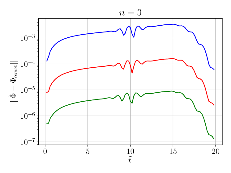
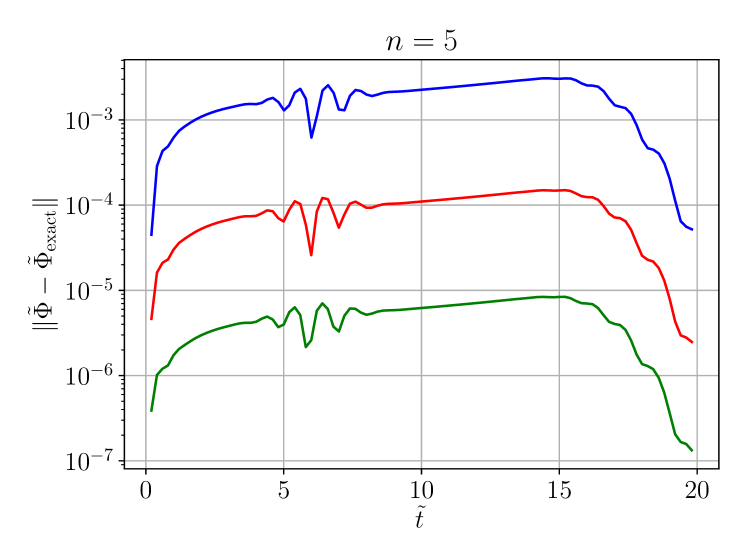
We now evolve these initial data and compare with the exact solution. In figure 1 we plot the norm of the error
| (60) |
as a function of time for three different radial resolutions at fixed angular resolution. We observe that doubling the resolution decreases the error nearly by a factor of , as expected for a fourth-order accurate finite-difference method.
We remark that at the chosen angular resolution, the spherical harmonics are represented exactly by our pseudo-spectral method, so there is no discretisation error in the angular dimensions for these linear evolutions.
4.2 Energy balance
In this section we derive and verify numerically the energy balance that the scalar field obeys on our hyperboloidal foliation. On standard slices of Minkowski spacetime approaching spacelike infinity, the energy (3) is conserved. In contrast, the energy computed on hyperboloidal slices decreases during the evolution. This is due to the fact that hyperboloidal slices intersect , so that outgoing waves pass through this conformal boundary, carrying away energy. We will compute this energy flux explicitly. A similar energy balance was derived in [10] in the context of linear scalar fields in Kerr spacetime, where an additional inner boundary arises at the black hole horizon.
The scalar field is associated with an energy-momentum tensor
| (61) |
where is the covariant derivative of the Minkowski metric . The vanishing of its divergence, , is equivalent with the NLW (29). The Killing vector gives rise to the conserved current
| (62) |
satisfying
| (63) |
Let denote the slice of constant hyperboloidal time with future-directed unit normal (normalised w.r.t. ) and induced Riemannian metric . Furthermore let denote the outward-directed normal to the timelike surface (again normalised w.r.t. ) and the induced pseudo-Riemannian metric on such a surface. Applying Gauss’ theorem to (63), the energy balance reads
| (64) | |||
| (65) |
where stands collectively for the angular coordinates on .
Expressing in terms of the conformally rescaled scalar field defined in 30, we obtain for the energy
| (66) |
Here refers to the gradient on and to its area element, e.g. for
| (67) |
In the first line of (4.2), we recognize the usual energy expression for the linear scalar field. The second line of (4.2) contains the contribution from the nonlinear potential, and the terms in the third line arise from the conformal rescaling.
The flux integral takes the form
| (68) |
It is is manifestly negative, reflecting the fact that the waves carry away energy as they pass through .
We now verify the energy balance numerically for two cases: (critical) and (supercritical). In both cases we impose an SO symmetry. The initial data are taken to be momentarily static with
| (69) |
and at implies
| (70) |
We superpose two modes with and and choose the parameters and . The amplitude for both modes is taken to be for and for , which is smaller than but close to the critical amplitude beyond which blow-up occurs in the focusing case (). The numerical resolution is taken to be .
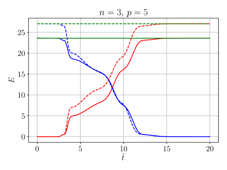
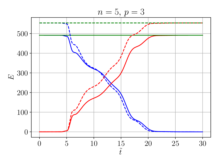
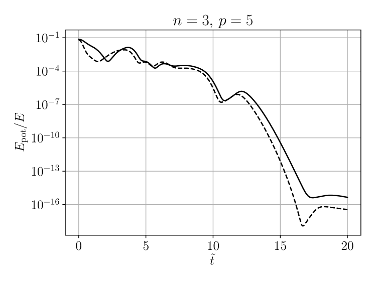
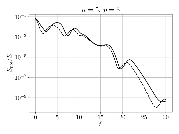
Figure 2 demonstrates that the energy balance
| (71) |
is well satisfied numerically, i.e., the sum of the numerically computed terms on the left-hand side is indeed nearly constant. For an evolution with a defocusing nonlinearity (), the initial energy is higher than for a focusing nonlinearity () due to the different sign of the potential energy term in (4.2).
We also compute this potential energy contribution alone,
| (72) |
and its ratio to the total energy, . The result is shown in figure 3 and indicates that the potential energy contribution becomes negligible at late times.
4.3 Tails
In this section we focus on the late-time behaviour of the scalar field, the so-called power-law tails. We extract the scalar field at various radii and decompose it into spherical harmonics. Each mode shows a characteristic power-law decay at late times. We investigate how the decay exponent depends on the power of the nonlinearity, the spherical harmonic mode indices and the extraction radius.
At a fixed extraction radius , we expand the scalar field in spherical harmonics, here in dimensions:
| (73) |
For each of the modes we form the local power index
| (74) |
If this approaches a constant as then the mode decays asymptotically as .
Our first observation is that the asymptotic decay rate appears to be independent of the azimuthal spherical harmonic index in three spatial dimensions. In order to illustrate this, figure 4 shows an evolution of static initial data (69)-(70) containing two modes with and . Via the nonlinearity (, focusing), modes with and are also excited during the evolution. The modes all decay at the same rate, irrespective of .
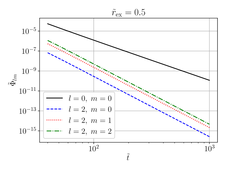
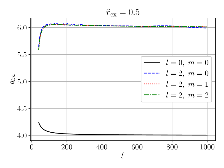
In the following we therefore focus on the case only, i.e. we impose axisymmetry for , and more generally an SO symmetry in dimensions.
In figure 5 we demonstrate convergence of the numerically computed local power index as the radial resolution is increased. In the following we will always choose the highest resolution shown here, and . We have checked that increasing the angular resolution has a negligible effect on the results.
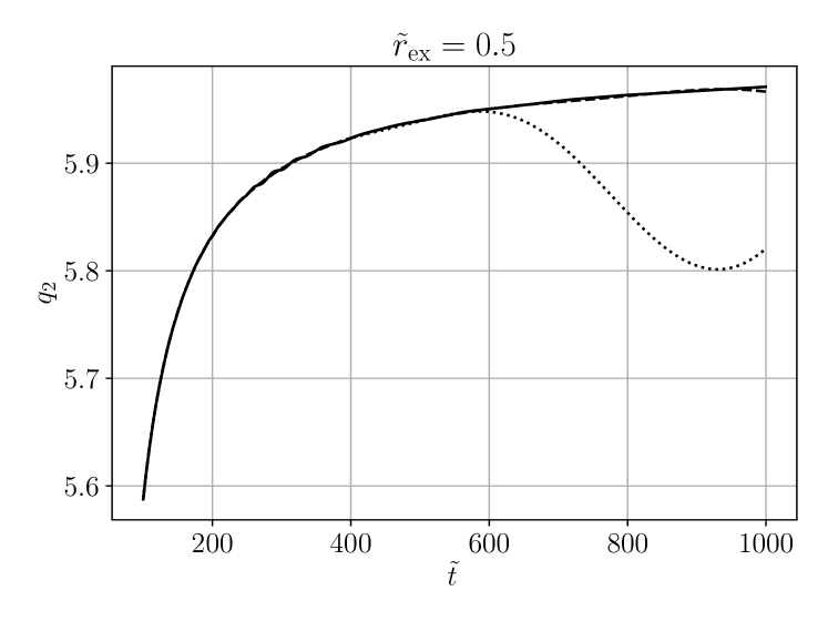
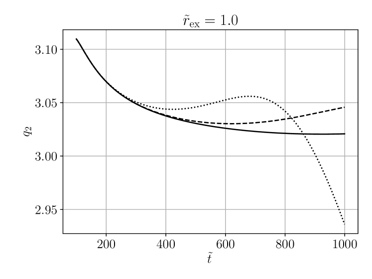
Next we compare the time evolution of the local power index at different extraction radii in figure 6. We observe that the local power index of a given mode approaches the same constant at all finite extraction radii, but in in general a different constant at ().
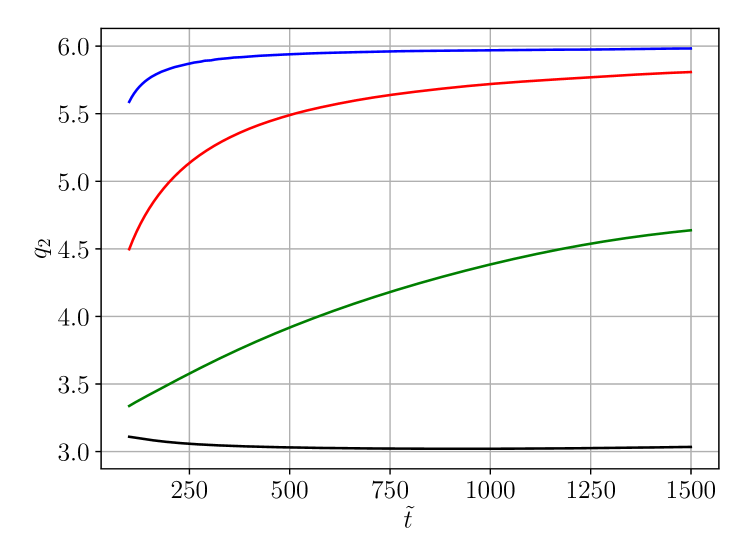
Finally we investigate the dependence of the decay rates on the spherical harmonic index . We show results for two selected cases, , focusing (figure 7) and , defocusing (figure 8). In the case the higher- modes are very small. We had to use higher precision (longdouble) for this run. Due to the smallness of the modes, computation of the local power index via (74) becomes numerically unstable. Instead, we have performed a power-law fit to the modes shown in figure 8 in order to obtain the decay rates.
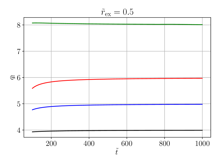
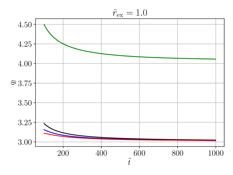
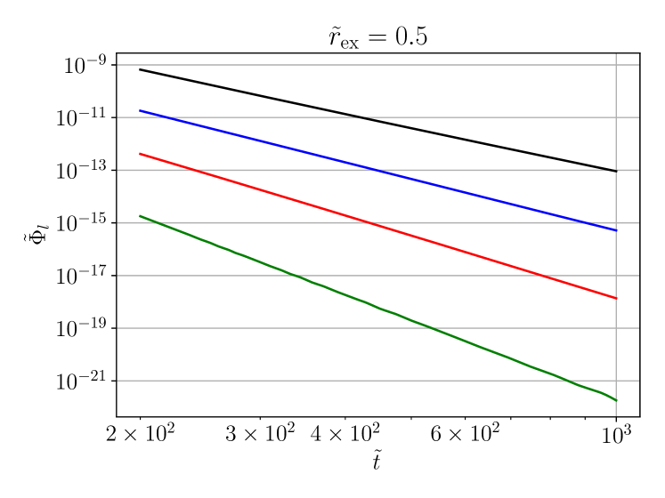
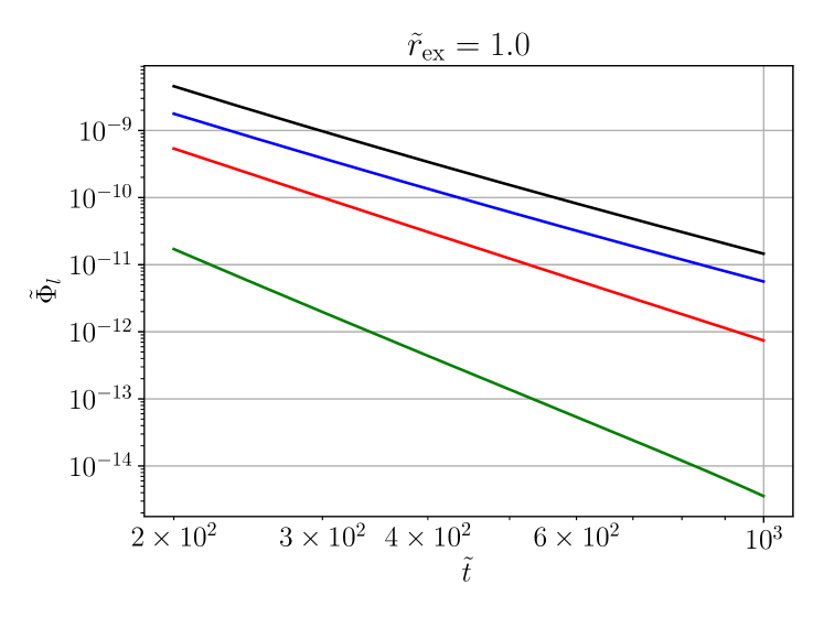
Table 2 summarises the asymptotic decay rates found in our numerical evolutions for and and various values of (subcritical and supercritical). We have compared focusing and defocusing evolutions and find the same asymptotic decay rates in both cases. In addition to the static initial data (69)–(70) used in the evolutions shown here, we have also tried different initial data taken from the exact linear solutions derived in A. The observed decay rates are identical. The static data have the advantage that they have an initially outgoing component so the tail forms earlier and with a higher amplitude than for the data from the linear solutions, which are initially ingoing.
5 Conclusion and discussion
This paper is concerned with the nonlinear wave equation
| (75) |
with , in spatial dimensions. Unlike previous studies, we do not assume radial symmetry. In we do not assume any symmetries, and in higher dimensions we impose an SO symmetry so that there is one effective angular coordinate.
We introduce a foliation of Minkowski spacetime into hyperboloidal slices of constant mean curvature, combined with a conformal compactification. This avoids the need for artificial timelike boundaries and allows us to numerically construct the solution in the entire future of the initial hyperboloidal slice, all the way up to future null infinity , where future-directed null gedodesics end.
Our numerical approach combines a fourth-order finite difference method in the radial coordinate with a Fourier pseudo-spectral method in the angular coordinate(s). We construct exact solutions to the linear wave equation and demonstrate fourth-order convergence of our code as the radial resolution is increased.
Unlike on standard slices approaching spatial infinity, the energy of the scalar field on hyperboloidal slices is not conserved. It decreases due to the energy flux at . We derive this energy balance and show that it is well satisfied in our numerical evolutions.
The main result of this paper concerns the late-time power-law decay of the solutions. We expand the evolved field into spherical harmonics and determine decay exponents of the individual modes for various values of the exponent of the nonlinearity (subcritical, critical and supercritical). The decay exponents appear to be the same for focusing and defocusing nonlinearities (). They are independent of the extraction radius as long as this radius is finite, but at different (smaller) decay rates are found. In three dimensions the decay exponents are found to be independent of the azimuthal spherical harmonic index , which justifies our assumption of axisymmetry or more generally SO symmetry. Our results in dimensions and are summarised in table 2.
At a finite radius, we would expect the scalar field to show the same decay in standard coordinates as in hyperboloidal coordinates . This leads us to the following
Conjecture 1
Consider the nonlinear wave equation (75) in spatial dimensions with , . Expanding the field in spherical harmonics
| (76) |
the modes decay asymptotically (as ) as
| (77) |
at any fixed finite radius . On slices approaching future null infinity , where , and the conformal factor , the conformally rescaled scalar field decays at asymptotically as
| (78) |
Indeed, this is consistent with [1], where the authors proved using perturbative methods that in spatial dimensions under spherical symmetry () and the solution decays asymptotically as at a finite radius. It would be very interesting to try and prove the above conjecture for .
In dimension , a similar form of the decay exponents consistent with table 2 would be
| (79) |
for the decay at a finite radius and at , respectively. More data would be needed to corroborate such a conjecture for though. This proves difficult numerically because the field decays very rapidly for higher exponents of the nonlinearity. Higher than longdouble precision would be needed.
Apart from tails, there are various other aspects of nonlinear wave equations that could be investigated using our hyperboloidal evolution code, in particular the nature of singularity formation (blow-up) and the threshold between blow-up and scattering. For example, this threshold was investigated numerically for the focusing cubic () wave equation in the subcritical dimension in radial symmetry in [7] (see also a similar study for the nonlinear Klein-Gordon equation [4]). In [18] the focusing cubic wave equation was considered in the supercritical dimensions and and again threshold solutions were identified. It will be interesting to analyse these situations beyond radial symmetry.
Appendix A Exact solutions, initial data
Here we work out exact solutions to the linear wave equation, which are used to test the convergence of the code in section 4.1. We first assume dimension without symmetries in A.1; higher dimensions will be treated in A.2. The solutions are constructed in standard spherical polar coordinates first; finally in A.3 they are transformed to hyperboloidal coordinates.
A.1 without symmetries
The solution to the linear wave equation
| (80) |
in standard spherical polar coordinates can be decomposed into spherical harmonics,
| (81) |
The spherical harmonics are eigenfunctions of the Laplace-Beltrami operator on ,
| (82) |
They have the form
| (83) |
where are the associated Legendre functions and are normalisation constants chosen such that
| (84) |
The (complex) spherical harmonics are implemented in scipy.special.sph_harm_y. A suitable real basis of spherical harmonics is obtained by taking
| (85) |
The wave equation implies that the radial functions in (81) obey an equation of Euler-Poisson-Darboux type,
| (86) |
Since this equation does not depend on explicitly, we leave out the index on in the following. Solutions have the form
| (87) |
where is an arbitrary mode function, and refers to an outgoing and to an ingoing solution. The coefficients can be determined by recursion. We provide explicit solutions for :
| (88) | |||||
| (89) | |||||
| (90) |
We observe that as is approached (, finite).
If we take the mode function to be odd and form the linear combination , the result turns out to be regular at the origin .
A.2 with symmetry
In this case we expand
| (91) |
where the real spherical harmonics are eigenfunctions of the Laplace-Beltrami operator on ,
| (92) |
We normalise them such that
| (93) |
where the area of is given in (57). The mode equation now reads
| (94) |
Note that for we recover (86).
In the following we state explicit solutions for . The first three spherical harmonics are
| (95) |
and the corresponding radial solutions are
| (96) | |||||
| (97) | |||||
| (98) |
We observe that now as is approached.
A.3 Transformation to hyperboloidal coordinates
From the conformal coordinates used in the code, we first compute the physical coordinates
| (99) |
so we can compute as constructed above. We then form
| (100) |
where the conformal factor is given by 16.
The multiplication by a negative power of in (100) may seem problematic at (), where . However, from the explicit solutions given in A.1 and A.2, we see that , and , so in (100) is in fact regular at .
For the initial data we also need to compute the field . By its definition, we have
| (101) |
with , and given in (16)–(18). Finally we need to express the derivatives of in terms of derivatives w.r.t. and :
| (102) |
where
| (103) |
The quantities and can be computed directly from the radial solutions (88)–(90) or (96)–(98).
References
References
- [1] Szpak N, Bizoń P, Chmaj T and Rostworowski A 2009 Linear and nonlinear tails II: exact decay rates in spherical symmetry J. Hyperbolic Differ. Equ. 6(1) 107–125
- [2] Strauss W and Vazquez L 1978 Numerical solution of a nonlinear Klein-Gordon equation J. Comput. Phys. 28(2) 271–278
- [3] Colliander J, Simpson G and Sulem C 2010 Numerical simulations of the energy-supercritical nonlinear Schrödinger equation J. Hyperbolic Differ. Equ. 7(2) 279–296
- [4] Donninger R and Schlag W 2011 Numerical study of the blowup/global existence dichotomy for the focusing cubic nonlinear Klein–Gordon equation Nonlinearity 24(9) 2547
- [5] Murphy J and Zhang Y 2020 Numerical simulations for the energy-supercritical nonlinear wave equation Nonlinearity 33 6195–6220
- [6] Frauendiener J 2004 Conformal infinity Living Rev. Relativity 7(1)
- [7] Bizoń P and Zenginoğlu A 2009 Universality of global dynamics for the cubic wave equation Nonlinearity 22(10) 2473–2485
- [8] Zenginoğlu A 2008 A hyperboloidal study of tail decay rates for scalar and Yang–Mills fields Class. Quantum Grav. 25(17) 175013
- [9] Rinne O and Moncrief V 2013 Hyperboloidal Einstein-matter evolution and tails for scalar and Yang-Mills fields Class. Quantum Grav. 30(9) 095009
- [10] Rácz I and Tóth G Z 2011 Numerical investigation of the late-time Kerr tails Class. Quantum Grav. 28(19) 195003
- [11] Csizmadia P, László A and Rácz I 2012 On the use of multipole expansion in time evolution of nonlinear dynamical systems and some surprises related to superradiance Class. Quantum Grav. 30(1) 015010
- [12] Harris C R et al. 2020 Array programming with NumPy Nature 585(7825) 357–362 https://numpy.org
- [13] Virtanen P et al. 2020 SciPy 1.0: Fundamental Algorithms for Scientific Computing in Python Nature Methods 17 261–272 https://scipy.org
- [14] Boyd J P 1978 The Choice of Spectral Functions on a Sphere for Boundary and Eigenvalue Problems: A Comparison of Chebyshev, Fourier and Associated Legendre Expansions Monthly Weather Rev. 106 1184–1191
- [15] Kreiss H O and Oliger J 1973 Methods for the approximate solution of time dependent problems (Global Atmospheric Research Programme Publication Series no 10) (Geneva: International Council of Scientific Unions, World Meteorological Organization)
- [16] Boyd J P 2000 Chebyshev and Fourier Spectral Methods (Dover Publications)
- [17] Fornberg B 1998 A practical guide to pseudospectral methods Cambridge Monographs on Applied and Computational Mathematics (Cambridge University Press)
- [18] Glogić I, Maliborski M and Schörkhuber B 2020 Threshold for blowup for the supercritical cubic wave equation Nonlinearity 33(5) 2143