A long-term study of Mrk 50 : Appearance and disappearance of soft excess
Abstract
We present an extensive temporal and spectral study of the Seyfert 1 AGN Mrk 50 using 15 years (2007-2022) of multiwavelength observations from XMM-Newton, Swift, and NuSTAR for the first time. From the timing analysis, we found that the source exhibited variability of 20% during the 2007 observation, which reduced to below 10% in the subsequent observations and became non-variable in the observations from 2010 onward. From the spectral study, we found that the spectra are nearly featureless. Non-detection of absorption in the low-energy domain during the 15 years of observation infers the absence of obscuration around the central engine, rendering the nucleus a ‘bare’ type. A prominent soft X-ray excess below 2 keV was detected in the source spectrum during the observations between 2007 and 2010, which vanished during the later observations. To describe the nature of the soft excess, we use two physical models, such as warm Comptonization and blurred reflection from the ionized accretion disk. Both the physical models explain the nature and origin of the soft excess in this source. Our analysis found that Mrk 50 accretes at sub-Eddington accretion rate () during all the observations used in this work.
1 Introduction
Active Galactic Nuclei (AGNs) are among the most luminous and energetic sources in the universe. The extremely high luminosity of the AGNs is understood to arise from the accretion of matter onto the supermassive black hole (SMBH) residing at the center of the host galaxies (Rees, 1984). The SMBH typically has a mass ranging from to M⊙ (Kormendy & Richstone, 1995; Peterson et al., 2004; Event Horizon Telescope Collaboration et al., 2019). The AGNs emit radiation across the entire range of the electromagnetic spectrum, from radio waves to high energy rays. According to the standard accretion disk theory (Shakura & Sunyaev, 1973), the thermal emission from the disk is mostly emitted in the ultraviolet (UV) band of the electromagnetic spectrum. Viscous dissipation in the disk generates heat, which is then radiated in the optical/UV regime for black hole masses typical of AGNs (Sun & Malkan, 1989). The X-ray emission from the AGN serves as an important tool for investigating physical processes in extreme gravity, as it is thought to originate from the innermost region of the accretion disk. The X-ray spectrum of AGN is primarily dominated by a power-law continuum produced through the inverse Compton scattering of the seed optical/UV photons from the accretion disk by a hot () optically thin corona (Shakura & Sunyaev, 1973; Haardt & Maraschi, 1993; Netzer, 2013) located near the black hole (Haardt & Maraschi, 1991; Narayan & Yi, 1994; Chakrabarti & Titarchuk, 1995; Done et al., 2007). The power-law continuum often shows a high-energy exponential cut-off, usually around a few hundred keV (Sunyaev & Titarchuk, 1980). This feature is directly related to the temperature and optical depth of the plasma of hot electrons responsible for the power-law emission. In addition to the power-law continuum with exponential cut-off, the other spectral features, such as reflection (Ross & Fabian, 1993, 2005; García et al., 2013, 2014), low energy absorption, and often an excess in the soft X-ray ranges (below 2 keV) (Halpern, 1984; Singh et al., 1985; Arnaud et al., 1985; Turner & Pounds, 1989), are also present in the X-ray spectra of the AGNs. The reflection features consist mainly of two components, such as a Compton hump, visible in the 15 to 50 keV range with a peak at around 30 keV (Krolik, 1999) and an iron emission line at 6.4 keV (George & Fabian, 1991; Matt et al., 1991). The origin of these reflection features can be due to the reprocessing of the primary X-ray continuum in the accretion disk and other neutral and ionized mediums around the central engine. The low energy absorption is typically significant in Seyert 2 AGNs, often due to dusty torus as described in the unification model (Antonucci, 1993). In contrast, the Seyfert 1s are usually not absorbed or only marginally absorbed with absorption column density, . The absence of strong absorption allows us to see an additional featureless spectral component, known as soft X-ray excess (below 2 keV) over the hard X-ray power-law continuum in many Seyfert 1s (Halpern, 1984; Arnaud et al., 1985; Turner & Pounds, 1989; Matzeu et al., 2020; Xu et al., 2021; Chalise et al., 2022). However, the origin of this spectral component has been a topic of research over the last years.
It was initially believed that the soft excess is originated from the inner part of the accretion disk as a hard-tail of the UV blackbody emission (Singh et al., 1985; Pounds et al., 1986; Leighly, 1999a; Magdziarz et al., 1998; Leighly, 1999b). However, this idea has been ruled out due to the high disk temperature ( keV) of a typical AGN accretion disk (Shakura & Sunyaev, 1973). In addition to that, different masses of the central black hole and different accretion rates for different AGNs indicate a wide range of disk temperature, which is inconsistent with the narrow range of disk temperature required to explain the soft excess observed in many sources (Gierliński & Done, 2004; Porquet et al., 2004; Piconcelli et al., 2005; Bianchi et al., 2009; Miniutti et al., 2009). The present understanding of the origin of soft excess favors either the warm Comptonizing corona model (Czerny & Elvis, 1987; Middleton et al., 2009; Done et al., 2012; Kubota & Done, 2018; Petrucci et al., 2018, 2020) or the blurred ionized reflection model (Fabian et al., 2002; Ross & Fabian, 2005; Crummy et al., 2006; García & Kallman, 2010; Walton et al., 2013). In the case of warm Comptonisation model, the optical/UV photons from the accretion disk are Compton upscattered in a warm ( keV) and optically thick corona covering the inner part of the disk, producing excess emission below keV (Czerny & Elvis, 1987; Done et al., 2012; Petrucci et al., 2018; Tripathi et al., 2019; Ursini et al., 2020; Middei et al., 2020). In the other model, the relativistically blurred and ionized reflection model predicts that the soft excess component is generated by the reprocessed hard X-rays from the hot corona in the inner disk. This processed emission produces several fluorescent atomic lines, which are blended and distorted due to the strong gravity of the black hole at the inner edge of the accretion disk (Jiang et al., 2018; García et al., 2019).
Markarian 50 (Mrk 50 ) is a Seyfert 1 galaxy at a redshift of (Vasudevan et al., 2013). Optical observations revealed that Mrk 50 exhibited significant variability in its nuclear region between 1985 and 1990, without any evidence of a disk structure in the system (Pastoriza et al., 1991). Mrk 50 is very bright in the X-ray range and known to be an unabsorbed Seyfert 1 galaxy with a soft excess and without any detectable iron line (Vasudevan et al., 2013). The first measurement of the black hole mass in Mrk 50, was determined by (Barth et al., 2011) using reverberation mapping technique and calculated the BH mass as M⊙. Using 2011 observation, Pancoast et al. (2012) reported the inclination angle of Mrk 50 to be deg, indicating that the system is close to face-on. They also estimated the mass of the central black hole to be . Bentz & Katz (2015) made a database of AGN black hole masses by compiling all published spectroscopic reverberation mapping studies of active galaxies and quoted the black hole mass in Mrk 50 as .
This work presents our findings from a comprehensive study of Mrk 50 using X-ray observations from various X-ray satellites. This paper is organized as follows. Section 2 provides an overview of the observations and outlines the procedures used for data reduction. Detailed analyses of the temporal and spectral behaviors of the source are presented in Section 3.1 and Section 3.2, respectively. Then, we discuss our key findings in Section 4, and finally, our conclusions are summarized in Section 5.
2 Observation and data reduction
Mrk 50 was observed with XMM-Newton (Jansen et al., 2001), Swift (Gehrels et al., 2004) and NuSTAR (Harrison et al., 2013) obervatories at different epochs. The publicly available data are reduced and analyzed using the HEAsoft v6.30.1 package. The details of the observations used in the present work are given in Table 1.
2.1 Swift
Swift (Gehrels et al., 2004) is a multi-wavelength satellite consisting of three onboard telescopes, operating in the optical/UV (Ultra-violet Optical Telescope; UVOT Roming et al. 2005), X-ray (X-ray Telescope; XRT Burrows et al. 2005) and hard X-ray (Burst Alert Telescope; BAT Barthelmy et al. 2005) wavebands. Mrk 50 was observed with Swift at several epochs from 2007 to 2022, with the most recent observation on 27 June 2022 in simultaneous with NuSTAR (see Table 1). We extracted the light curves and spectra from the observed data by using the web tool ‘XRT product builder’111http://swift.ac.uk/user_objects/(Evans et al., 2009). Additional finer steps, such as pile-up correction on the given observation ID/IDs, are also applied while using the web tool. The tool processes and calibrates the data and produces final spectra and light curves of Mrk 50 in two modes, e.g., window timing (WT) and photon counting (PC) modes. In 2007, Swift observed Mrk 50 in three consecutive days from 14 November 2007 to 16 November 2007 with XRT for exposure times of ks, ks, and ks, respectively. Due to the short exposures, the signal-to-noise ratios (SNR) during these observations are poor. The hardness ratios (ratio between count rates in the 1.5–10 keV and the 0.3–1.5 keV band) were also found to be unchanged during these observations. We, therefore, considered these three observations together and produced a combined observation (S1) for an exposure time of ks.
The Swift/UVOT provides data in three optical filters (V, B, and U) and three UV filters( UVW1, UVM2, and UVW2). We started our UVOT data reduction from the level II image files, performing photometry using the tool UVOTSOURCE. To obtain the source counts, we assumed a circular region of 5 arcsec radius centered at the source position, whereas a circular region with 20 arcsec radius, away from the source position, was considered for background counts. We used the UVOT2PHA tool to create XSPEC-readable source and background spectra and used response files provided by the Swift team. In this work, we used only data from the UV filters (UVW1, UVM2, and UVW2) and excluded the optical (V, B, and U) data due to the contribution from the host galaxy and starburst in this band.
For Swift/BAT, we downloaded the hard X-ray spectrum of Mrk 50 from the 105-Month Swift/BAT All-sky Hard X-Ray Survey222https://swift.gsfc.nasa.gov/results/bs105mon/. In addition, a response matrix appropriate for the BAT spectra was used in our work.
| ID | Date | Obs. ID | Observatory | Instrument | Exposure |
|---|---|---|---|---|---|
| (yyyy-mm-dd) | (ks) | ||||
| S1 | 2007-11-14 | 00037089001 | Swift | UVOT & XRT | 20.4 |
| –2007-11-16 | –00037089003 | ||||
| X1 | 2009-07-09 | 0601781001 | XMM-Newton | OM, RGS, PN & MOS | 11.9 |
| X2 | 2010-12-09 | 0650590401 | XMM-Newton | RGS, PN & MOS | 22.9 |
| S2 | 2013-12-27 | 00080077001 | Swift | UVOT & XRT | 6.5 |
| S3 | 2022-06-27 | 00080077002 | Swift | UVOT, XRT & BAT | 5.7 |
| NU | 2022-06-27 | 60061227002 | NuSTAR | FPMA & FPMB | 17.4 |
2.2 XMM-Newton
XMM-Newton (Jansen et al., 2001) observed Mrk 50 at two epochs in July 2009 and December 2010. The details of the observations are mentioned in Table 1. Data from the European Photon Imaging Camera (EPIC), Reflection Grating Spectrometer (RGS) and Optical Monitor (OM) instruments are used in the present work. The EPIC includes three X-ray CCD cameras covering the 0.3 – 10 keV energy bandpass: two Metal Oxide Semiconductors (MOS1 and MOS2; Turner et al. (2001)) and a p-n CCD (PN; Strüder et al. (2001)). The two RGS detectors (RGS1 and RGS2) provide high-resolution spectroscopy over the 0.35–2 keV energy range (den Herder et al., 2001). The OM (Mason et al., 2001) provides photometric data from optical to UV bands (U, B, V, UVW2, UVM2, and UVW1).
We analyzed the Observation Data File (ODF) using XMM-Newton Science Analysis System () and updated calibration files as of 23 October 2019. We processed all the EPIC data using the tasks and to obtain the calibrated and integrated event lists for the MOS and PN detectors, respectively. We filtered the data using the standard filtering criterion. Data during high background flaring events were removed before extracting the spectral products by creating and choosing appropriate good time intervals () using the task . In this work, we considered only the unflagged events with PATTERN and PATTERN for the PN and MOS detectors, respectively. The data were checked for photon pile-up using the task and corrected accordingly. The source photons were extracted by considering an annular region with outer and inner radii of 30 and 5 arcsecs, respectively, centered at the source coordinates. We used a circular region of 60 arcsec radius, away from the source position, for the background products. The response files for PN and MOS detectors were generated using tasks and for arf and rmf files, respectively.
We reduced the RGS data using the standard task and the updated calibration files to produce the source and background spectra. The cleaned event lists were generated by applying the standard filtering criteria. The response matrices were generated using the task. The individual RGS1 and RGS2 spectra were combined into a single merged spectrum using the task to achieve better signal-to-noise for the purpose of spectral fitting.
The Optical Monitor (OM) (Mason et al., 2001) was also used simultaneously to observe Mrk 50 in 2009 in imaging mode with UVW1 and UVW2 filters. For the 2010 observation (0650590401), however, the optical/UV data from the OM are not available. We processed the OM data using the task . The command was used to generate -readable spectral files for all the available filters. For the OM data, we used the canned response files available in the ESA XMM-Newton website333https://sasdev-xmm.esac.esa.int/pub/ccf/constituents/extras/responses/OM/. We obtained background corrected count rates from the source list for each OM filter and converted the count rates into respective flux densities444https://www.cosmos.esa.int/web/xmm-newton/sas-watchout-uvflux.
2.3 NuSTAR
NuSTAR is a hard X-ray focusing telescope consisting of two identical focal plane modules, FPMA and FPMB, and operates in the 3–79 keV energy range (Harrison et al., 2013). Mrk 50 was observed with NuSTAR simultaneously with Swift in June 2022. The observation details are presented in Table 1. We use standard NuSTAR Data Analysis Software (NuSTARDAS v2.1.2555https://heasarc.gsfc.nasa.gov/docs/nustar/analysis/) package to extract data. The standard NUPIPELINE task with the latest calibration files CALDB 666http://heasarc.gsfc.nasa.gov/FTP/caldb/data/nustar/fpm/ is used to generate the cleaned event files. The NUPRODUCTS task is utilized to extract the source spectra and light curves. We consider circular regions of radii 60 and 120 arcsecs for the source and background products, respectively. The circular region for the source is selected with the center at the source coordinates, and the region for the background is chosen far away from the source to avoid contamination.
3 data analysis and result
3.1 Timing analysis
We conducted the timing analysis of Mrk 50 using light curves from the Swift/XRT, XMM-Newton, and NuSTAR observations (see Table 1). The time resolution of the light curves used in our analysis is 200 s. The light curves in the 0.3-10 keV range, generated from the XMM-Newton and Swift/XRT observations, and in the 3-60 keV range from NuSTAR are shown in Figure A1. Further, we extract light curves in the soft (0.3–3 keV range) and hard (3-10 keV range) X-ray bands for the variability and correlation studies. The light curve obtained from the NuSTAR observation is used to explore the variability of the source in the high-energy domain (3–60 keV). The entire energy range (3–60 keV) is further subdivided into two energy bands: band 1 (3–10 keV) and band 2 (10–60 keV), for variability studies.
3.1.1 Fractional Variablity
To check the temporal variability of Mrk 50 across different energy bands, we calculate the fractional variability (Edelson et al. 1996; Nandra et al. 1997; Rodríguez-Pascual et al. 1997; Vaughan et al. 2003; Edelson & Malkan 2012). The fractional variability for a light curve of counts/s with the measurement error for number of data points, mean count rate and standard deviation , is given by the relation,
| (1) |
where, is the excess variance (Nandra et al. 1997; Edelson et al. 2002), used to estimate the intrinsic source variance and given by,
| (2) |
The normalized excess variance is defined as . The uncertainties in and are estimated as described in Vaughan et al. (2003) and Edelson & Malkan (2012). The peak-to-peak amplitude is defined as (where, and are the maximum and minimum count rates, respectively) to investigate the variability in the X-ray light curves.
During the 2007 observation (S1), we found that the average count rate and the peak-to-peak amplitude remain constant at count s-1and for both the soft X-ray and the entire energy bands, respectively. In these energy bands, the normalized excess variance () and corresponding fractional variability () are found to be constant at and , respectively. For the hard X-ray band, the average count rate, , decreases to count s-1, and the corresponding value increases to . In this energy band, the fractional variability () is estimated to be . So, in this epoch (S1), the source was variable () in the soft X-ray, hard X-ray, and the entire energy band. The average source count rate was maximum during the 2009 and 2010 XMM-Newton observations (X1 & X2) compared to the epochs of other observations used in the present work. While estimating the fractional variability (), we find that in all the energy bands, is . This indicates that the source was non-variable during these observations. For S2, S3 and NU observations, the variability parameters like and are also calculated. However, due to the low count rate and high error associated with each data point, we encounter negative values for normalized excess variance, resulting in imaginary fractional variability. The details of the results of the variability analysis are presented in Table 2.
| ID | Energy | |||||||
|---|---|---|---|---|---|---|---|---|
| keV | count | count | count | () | ||||
| S1 | 0.3-3 | 122 | 0.87 | 0.19 | 0.50 | 4.57 | 5.171.07 | 22.742.78 |
| 3-10 | 118 | 0.31 | 0.02 | 0.09 | 14.44 | 3.774.54 | 19.4211.77 | |
| 0.3-10 | 122 | 1.04 | 0.23 | 0.58 | 4.47 | 4.311.81 | 20.772.68 | |
| X1 | 0.3-3 | 50 | 9.87 | 8.30 | 9.01 | 1.20 | 0.05 0.02 | 2.260.56 |
| 3-10 | 50 | 0.72 | 0.39 | 0.55 | 1.87 | 0.300.31 | 5.492.95 | |
| 0.3-10 | 51 | 10.38 | 8.79 | 9.55 | 1.18 | 0.040.02 | 2.000.60 | |
| X2 | 0.3-3 | 105 | 5.78 | 4.25 | 5.02 | 1.36 | 0.270.04 | 4.790.56 |
| 3-10 | 106 | 0.64 | 0.25 | 0.42 | 2.52 | 0.530.40 | 7.272.78 | |
| 0.3-10 | 104 | 6.21 | 4.63 | 5.44 | 1.34 | 0.230.04 | 4.870.05 |
Note: In most of the cases (S2, S3 and NU observation), the average error of the observational data surpasses the 1 limit,
resulting in negative excess variance. As a result, these cases contain imaginary values for , and thus, they are excluded
from the table.
3.1.2 Cross-correlation
We carried out the cross-correlation function (CCF) analysis to search for a correlation and time lag between X-ray light curves in different energy bands. We applied the -transformed discrete correlation function (DCF777www.weizmann.ac.il/particle/tal/research-activities/software) method (Alexander, 1997, 2013) to estimate the CCF between the light curves. This method is suitable for both evenly and unevenly sampled data but is particularly appropriate when the observed data are unevenly sampled and sparse. However, the ZDCF binning algorithm uses a logic similar to that of the discrete correlation function (DCF) developed by Edelson & Krolik (1988). However, the ZDCF method adopts equal population binning and Fisher’s z-transform to correct several biases of the DCF method. We used the available FORTRAN 95 888https://www.weizmann.ac.il/particle/tal/research-activities/software code to carry out the cross-correlation. While performing the ZDCF analysis, we used 102000 Monte Carlo runs for the error estimation of the coefficients. Also, we did not consider the points for which the lag was zero. The X-ray light curves in different energy bands from different observations are shown in the upper panels of Figure 1. Furthermore, we plot the correlation function between the light curves of different energy bands in the middle panels of Figure 1. The count–count plots are also presented in the bottom panels of the same figure.
To probe the origin of the soft excess in Mrk 50, we investigate the time delay between the soft X-ray (0.3–3 keV) and hard X-ray (3–10 keV) bands using the cross-correlation method. We begin our analysis using data from observation S1 and find that the soft and hard X-ray bands are uncorrelated. We find similar results in the case of observations X1 and X2. We do not notice any significant peak in the discrete cross-correlation function in any of the observations (see Figure 1). The detection of no correlation between soft and hard X-ray bands suggests that the photons in both energy bands could have originated through different physical mechanisms. We then investigate the correlation between the light curves in the high-energy regime. Light curves from the NU observations in band1 and band2 are utilized to explore the correlation in the high-energy regime. In this case, we find that these two bands are uncorrelated. The details of our findings from the cross-correlation study are explained in section 4.4.2.


3.2 Spectral Analysis
The spectral analysis is carried out using Swift (XRT & UVOT) and XMM-Newton (EPIC-pn, MOS & OM) observations in 0.001-10 keV range and simultaneous Swift (UVOT, XRT & BAT) and NuSTAR observations in 0.001–120 keV range (see Table 1). The NuSTAR data beyond 60 keV are not considered in the present analysis as it is dominated by background. We use XSPEC v12.12.1 (Arnaud, 1996) software package for spectral fitting. We binned the spectral data at a minimum of 25 counts/bin for both XMM-Newton and NuSTAR observations and 20 counts in each bin for the Swift/XRT observations. The GRPPHA task is used for binning the spectral data. The model likelihoods are determined using the statistic. However, it is to be noted that the Swift/BAT data are Gaussian999https://swift.gsfc.nasa.gov/analysis/threads/batspectrumthread.html, and we continue to present the -statistic here for simplicity. We also ignored the bad channels in our analysis.
The best-fit parameters are reported in the rest frame of the source. The uncertainties corresponding to the model parameters are quoted at the 90% confidence level using the Monte Carlo Markov Chain (MCMC) method embedded in . The MCMC technique simultaneously determines the errors in the model parameters and renders better parameter space sampling than other methods. We used the Goodman & Weare sampler (Goodman & Weare, 2010) to deal with degeneration in the model parameters. For sampling, we choose the number of walkers to be more than twice the number of free model parameters. In all cases, we consider the chain length of 200000 for the chains to converge in the same parameter values. The first 10000 steps are discarded for the burn-in period to remove the bias introduced by the choice of the starting location. To ensure that the walkers have enough sampling in the parameter space, we checked whether the steps were rejected less than 75% of the time or not.
The unabsorbed X-ray luminosity from each spectrum is estimated using clumin task on the powerlaw model. While estimating the luminosity, we use the redshift, =0.023. We also calculate the X-ray flux by using cflux command in XSPEC. The observed UV flux is corrected for reddening and Galactic extinction using the reddening coefficient obtained from the Infrared Science Archive 101010http://irsa.ipac.caltech.edu/applications/DUST/ and following Schlafly & Finkbeiner (2011). The Galactic extinction () value used is . The X-ray and UV monochromatic flux are quoted in Table 7. Throughout this work, we use the Cosmological parameters as follows: (Bennett et al., 2003).

3.3 Characterising the spectrum
As Mrk 50 has not been explored in the high-energy domain to date, our first motivation is to characterize the spectrum of this source. For this purpose, we begin our spectral fitting with a set of phenomenological models to characterize the source spectra at different epochs and determine the spectral features quantitatively. Further, these phenomenological models are replaced with more sophisticated physical models to better understand the physical properties of the source.
Initially, we consider the 3–10 keV X-ray continuum spectra of the source for the spectral fitting. According to current understanding, the X-ray continuum photons are produced through the inverse Compton scattering of thermal photons from the accretion disk in a hot electron cloud (Shakura & Sunyaev, 1973), though the geometry and location of this hot electron cloud are poorly understood. This non-thermal process leads to a power-law-type spectrum. Therefore, we applied a simple Powerlaw model to fit the spectrum of each observation. Along with this, we use the Galactic line of sight hydrogen column density () as the multiplicative model TBabs (Wilms et al., 2000) in XSPEC. The value of 111111https://heasarc.gsfc.nasa.gov/cgi-bin/Tools/w3nh/w3nh.pl used in our work is . We note that we did not observe any prominent (positive) residual in the 6–7 keV energy range during the continuum fitting of any of the five sets of spectra (see left panel of Figure 2). This indicates the absence of the Fe-line in the X-ray continuum of Mrk 50. So, for the continuum, the baseline model is for all observations. The Constant component is used as a cross-normalization factor while using data from different instruments in simultaneous spectral fitting (see Table A1).
After successfully parameterizing the primary continuum in the 3-10 keV range, we extend the spectrum into the low-energy domain (below 3 keV), where we find distinct results across different epochs of observations (see right panel of Figure 2). In the case of S1, we notice deviation in the low-energy data points from the primary continuum, which is attributed to the presence of soft excess at . To address the presence of soft excess in this observation, we consider another power-law component below 3 keV (Walter & Fink, 1993; Nandi et al., 2021). To ensure the significance of this additional component, we conducted an F-test121212https://heasarc.gsfc.nasa.gov/xanadu/XSpec/manual/node82.html for the additive component, and find the to be 9.86 with a probability of chance improvement . Using the F-test, we verified that an additional component is required. We also find evidence of soft excess in X1 & X2 observation.
However, for observations S2 and S3+NU, it is surprising that the low energy spectra (below 3 keV) do not show the presence of any excess emission over the continuum. The primary continuum fits the extended low energy range of these observations. The exposure times for S2 and S3 observations are shorter compared to the other observations, which may explain the non-detection of the soft excess component below 3 keV. However, for further clarification, we performed an F-test on these spectra. The F-test confirms that adding the extra power-law component is insignificant and did not improve the fit.
To investigate the presence of any intrinsic absorption along the line of sight of Mrk 50, we initially used the neutral absorption model component, zTbabs, with our baseline model and found that the estimated value of is for . To investigate further, we replace zTbabs with a partially covering absorption model Pcfabs to check for the presence of any partial absorbers present in the line of sight. However, this model is also found to be insensitive during spectral fitting and consistently yields the lowest value of the absorption parameter. We considered UV data for these observations in our spectral fitting to ensure our findings. However, the inclusion of UV data in the fitting did not detect the presence of any extragalactic absorption component in Mrk 50. As a result, we drop this zTbabs component from our composite model. The corresponding model in XSPEC read as and is used to fit all the spectra in the 0.3 – 10 keV range. Later, we extend the low energy part into the UV domain whenever the UV observations are available.
In the high energy domain (10 keV), we combine spectra from the Swift/XRT, NuSTAR, and Swift/BAT to obtain a broad-band X-ray spectrum up to 100 keV. While extrapolating the primary continuum model to the high-energy range, we did not find any deviation in the data points from the primary model (see Figure 2). This suggests that the reflection component in the X-ray spectra above 10 keV is either absent or insignificant during this observation.
After characterizing each spectrum of all the observations with simple models, such as power-law, we use the phenomenological model Diskbb to address the soft X-ray excess (see Section 3.3.3) in this source. To better understand the physical nature of the soft X-ray excess emission in Mrk 50, we use Optxagnf and Relxillcp as physical models. The results are discussed in the following sections.
3.3.1 RGS spectral analysis
Before proceeding to a detailed spectral analysis of the source, we first present a brief analysis of the RGS data to confirm the ’bare’ nature of Mrk 50. We analyzed the merged RGS spectrum (RGS1+2) of Mrk 50 to check for possible prominent soft X-ray absorption and/or emission in the energy range of 0.4-2 keV. We adopt the spectral binning of 20 counts/bin and use the statistics. The merged RGS spectrum is initially modeled by simple powerlaw modified by the Galactic absorption. The absorbed power-law model provided a good fit with -statistic of 407.52 for 395 degrees of freedom and of for the X1 observation. For X2 observation, we found -statistic of 299.43 for 320 degrees of freedom and of . Figure 3 shows the absorbed power-law fitted merged RGS spectra of Mrk 50 for both the XMM-Newton observations (X1 & X2), with the residual shown in the lower panel. To investigate the presence of any ionized absorption, we used the multiplicative model Zxipcf to the power-law model. This addition resulted in an insignificant improvement in the fit statistics. The upper limit of the column density was constrained to for X1 observation. However, this model was also found to be insensitive during spectral fitting of X2 observation. Such a lower value of the was previously seen in other systems (Laha et al., 2014; Matzeu et al., 2020; Nandi et al., 2024; Madathil-Pottayil et al., 2024; Porquet et al., 2024). This indicates that no significant warm absorbing gas exists along our line of sight towards this AGN, thereby supporting its classification as a bare Seyfert 1 galaxy.

.
ID
()
log ( erg s-1)
()
log( erg s-1)
S1
260.93/203
X1
1864.48/1597
X2
1894.17/1725
S2
73.95/84
S3+NU
238.61/196
in the unit of photons/keV/cm2/s.
3.3.2 Powerlaw
We started our spectral analysis with an absorbed power-law model as described in Section 3.3. From the spectral fitting, we found that the power-law indices of the primary continuum () varied from to and the corresponding luminosities () varied from to . After the primary continuum fitting, we fitted the lower energy range (below 3 keV) of the observed spectrum using another power-law component (see section 3.3). We considered available UV data in the spectral fitting, and used the multiplicative model Redden (Cardelli et al., 1989) with a fixed value of (Schlafly & Finkbeiner, 2011) to account for the inter-stellar extinction. The model for spectral fitting of data in the 0.001 to 10 keV range is represented in XSPEC as .
For the 2007 observation (S1), we found the power-law indices of soft excess and the primary continuum are in the same order. This indicates a minimum presence of soft excess in this observation period. We also calculated the corresponding luminosities and found that these values are nearly the same. The primary continuum luminosity for S1 is calculated as erg s-1, whereas, the soft excess luminosity is erg s-1. From X1 (2009) and X2 (2010) XMM-Newton observations, we found a difference in and along with the luminosities, indicating a strong presence of soft excess in these two observations. The deviation from the primary power-law continuum below 3 keV is significant in X1 (see Figure 2), which is characterized by . In X2, the amount of soft excess is reduced, but a significant presence of this component is still observed with .
After three years of XMM-Newton observations, Mrk 50 was observed with Swift in 2013 (S2) in UV and X-ray bands. In this observation (S2), we could not detect the soft excess emission below 3 keV. As a result, the values of power-law indices are found to be in the same order (within uncertainties). and are and , respectively, for this observation.
In 2022 (S3+NU), a broadband simultaneous observation of the AGN was carried out with Swift (UVOT, XRT, and BAT) and NuSTAR . Although the spectrum is extended to 100 keV, initially, we considered data up to 10 keV from Swift (UVOT and XRT) and NuSTAR for the powerlaw+powerlaw model fitting. During the spectral fitting, the soft excess was barely detectable (see Figure 2), for which we could not constrain the power-law index and corresponding luminosity of the soft excess. We fixed at , same as , and corresponding luminosities are estimated to be erg s-1 and erg s-1 for and , respectively. It is to be noted that we are unable to calculate the errors in soft excess luminosity as the is fixed at 1.77. The values of the parameters obtained from spectral fitting are presented in Table 3.
3.3.3 Diskbb
After parameterizing the soft excess component by a simple power-law component, we started characterizing this excess using a multi-temperature accretion disk blackbody model Diskbb (Mitsuda et al., 1984). The Diskbb is a relatively simple model with only two model parameters: the temperature at the inner edge of the disk and the model normalization. This model describes the data well in the optical/UV band. Therefore, we used simultaneous UV and X-ray data to investigate the soft excess in UV and X-ray spectra. For the spectral fitting, the model in XSPEC reads as .
From the S1, we found that the inner disk temperature () is keV with power-law index of . A similar approach is followed for the spectral fitting of data from X1 and X2. As the soft excess is strong in these observations, we are able to constrain the inner disk temperature . We found that the inner disk temperatures, (), are and for X1 and X2, respectively. The power-law indices () are calculated as and for the corresponding observations.
In the case of S2 and S3+NU, as the presence of soft excess is below the limit of detection, we are unable to draw a limit on the inner disk temperature () of the Diskbb component. So, we fixed the value of at keV. As the values of s are not constrained to a certain limit, we are unable to limit the normalization of this model component. For the other model component (Powerlaw), we found the photon indices () are and for the S2 ad S3+NU, respectively. The values of the best-fit parameters and their fit statistics are quoted in Table 4.

3.4 The physical models
In this section, our motivation is to understand the physical origin of each spectral component and its evolution over time. The origin of the soft excess component is yet to be understood. To explore this, we considered two possible physical scenarios, warm Comptonization (Done et al., 2012) and relativistic blurred reflection (García et al., 2018), on the observed spectra to investigate the physical origin of this component.
3.4.1 Warm Comptonization
In this scenario, we used Optxagnf (Done et al., 2012) model as the warm Comptonization model to investigate the origin of soft excess in this source. It is an intrinsic thermal Comptonization model that describes the optical/UV emission of AGNs as multicolor blackbody from a colour temperature-corrected disk. In this model, the disk emission emerges at radii , where and are the outer edge of the disk and the corona, respectively. At , the disk emission emerges as the Comptonized emission from a warm and optically thick plasma, expressed as the soft X-ray emission (Magdziarz et al., 1998; Done et al., 2012). The hot and optically thin corona is considered to be located around the disk and produces the high-energy power-law continuum. The observed Comptonized emission, therefore, consists of contributions from the cold and hot corona, with the fraction of hot-Comptonized emission determined by a parameter, , obtained from the model fitting.
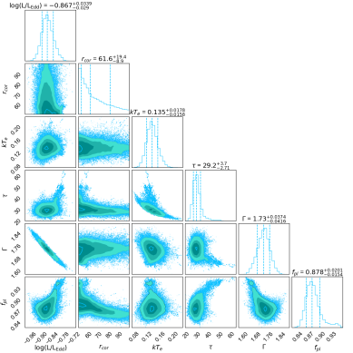
This model characterizes the total emission based on the mass accretion rate and the black hole mass. The soft X-ray excess emission is determined by parameters such as the temperature of the warm corona ( ), the temperature of the seed photon, and the optical depth of the warm corona () at . The power-law continuum is approximated as the nthcomp model, with the seed photon temperature fixed at the disk temperature at and the electron temperature fixed at 100 keV. Four parameters that determine the model flux are the black hole mass (), the Eddington ratio (), the moving distance (D in Mpc), and the dimensionless black hole spin (a). While using the Optxagnf model, we kept the black hole mass of Mrk 50 fixed at (Bentz & Katz, 2015) and the cosmological distance at 103 Mpc. As recommended, we fixed normalization to unity during our analysis.
| ID | ||||||
|---|---|---|---|---|---|---|
| (keV) | () | () | ||||
| S1 | 213.50/202 | |||||
| X1 | 1574.47/1596 | |||||
| X2 | 1836.74/1724 | |||||
| S2 | 77.19/84 | |||||
| S3+NU | 322.16/282 |
Notes: Spectral fitting of all observations include simultaneous
optical-UV data except X2.
in the unit of photons/keV/cm2/s.
indicates a frozen parameter.
The warm Comptonization model uses the disk UV photons to produce the power-law continuum spectrum and the soft excess. Therefore, to constrain the Optxagnf parameters, we fitted the X-ray data along with simultaneously obtained UV data from the XMM-Newton and Swift observations, except for X2, where no UV data was available. The Redden model in XSPEC accounts for galactic extinction correction. During our analysis, the black hole spin parameter could not be well constrained when kept as a free parameter. Hence, we fixed the spin value at the maximal spin scenario (=0.998) in the fitting process.
From the spectral fitting of S1 data, we found that the accretion rate () is , with corresponding warm corona temperature () and optical depth () of keV and , respectively.In this observation, the soft excess emission is not prominent, and we found the coronal boundary () to be at . The hard X-ray part of this spectrum is characterized by the power-law with index () of . The corresponding fraction of the energy below emitted in the hot corona is , while the fraction emitted in the warm corona is . In the 2009 observation (X1), the accretion rate decreased to , leading to a warm corona temperature of keV and an optical depth of . As the soft excess is prominent in this observation, we found that gets extended up to . From the spectral fitting, we determined to be with .
In the next observation in 2010 (X2) with XMM-Newton, we found that the accretion rate further decreased to with corresponding as . The warm corona is characterized by and , which are found to be keV and , respectively. Notably, this observation exhibited the highest temperature of the warm corona. For this observation, and are found to be and , respectively.
In the 2013 (S2) and 2022 (S3+NU) observations, as the soft excess was not detected in the spectral fitting, it is difficult to fit the spectra using the Optxagnf model. During fitting, most of the model parameters were insensitive. Therefore, we could not constrain them to a significant limit. We started our fitting by fixing the warm corona temperature at keV for both observations. It is important to note that this is the lower limit of , and the model is insensitive to this parameter. We also calculated the upper limit of the optical depth and coronal radius for these observations. Additionally, the fraction of energy emitted as the power-law component () was constrained to an upper limit of for both observations. The photon indices for these observations are found to be and , respectively. The values of the best-fitted parameter are quoted in Table 5. We show in Figure 5 the results of the MCMC analysis for the best-fit Optxagnf model parameters found from the S1 and X1, and the best fitting spectrum along with the residuals presented in Figure 6.

3.4.2 Relativistic Reflection
Another possible origin of the soft X-ray excess is the relativistically blurred reflection from a photo-ionized accretion disk (García et al., 2019; Matzeu et al., 2020; Ghosh & Laha, 2020; Xu et al., 2021; Ghosh et al., 2022; Kumari et al., 2023; Yu et al., 2023). When emission from the primary continuum originating from the corona or Compton cloud illuminates the colder accretion disk, a reflection spectrum with fluorescence lines and other spectral features is produced (Ross & Fabian, 2005). These emission lines are then blurred and distorted by relativistic effects (Laor, 1991; Crummy et al., 2006) as they originate close enough to the supermassive black hole. This process can generate a smooth spectrum below 2 keV, commonly called soft excess.
To investigate the presence of relativistic reflection in the spectra of Mrk 50, we adopted the Relxillcp model (García et al., 2018), a variant of the relativistic reflection model Relxill (García et al., 2013, 2014; Dauser et al., 2014, 2016). The Relxillcp model uses the nthcomp model (Zdziarski et al., 1996; Życki et al., 1999) as a simple Comptonization model to calculate the primary source spectrum. This variant does not assume any particular geometry, and the primary continuum emission is characterized by the spectral index () and the temperature of the corona ().
The reflection fraction , a parameter of the Relxillcp model, is defined as the ratio between the Comptonized emission directed towards the disk and that escaping to infinity. The emission profile is modeled as a broken power-law with for and for , where , , , and represent the emissivity, outer emissivity index, inner emissivity index, and break radius, respectively. This model also provides information on parameters such as the ionization parameter (), iron abundance (), inclination angle (), the inner radius of the accretion disk (), and the spin parameter of the black hole .
During spectral fitting, we initially fixed the black hole spin parameter to the maximum value and set the inner radius () to , the lowest value allowed in the model. In the second scenario, we fixed the spin parameter to zero and set the inner radius to . The fit statistics did not improve for the rotating or non-rotating scenarios across all our observations. The maximally spinning black hole scenario has also been observed in previous studies in other Seyfert 1 galxies (García et al., 2019; Waddell et al., 2019; Xu et al., 2021). Therefore, we continued with the rotating black hole scenario for spectral fitting, and we kept the spin parameter and inner radius fixed at and , respectively.
We start our analysis using the Relxillcp model and find that this model alone could not fit all the observed spectra from UV to X-ray bands. While it fits the spectra above 0.3 keV for all observations, it does not account for the lower-energy UV spectra. We added a power-law component to the model to fit the broadband spectra from UV to X-ray ranges for all observations. Therefore, the model used to fit the broadband spectra from UV to X-ray is represented as . The fitted results are presented in Table 6. In our analysis, the emissivity index (), which corresponds to the geometry of the accretion disk in the outer region , was fixed at . As a result, the outer portion of the disk behaves like a Newtonian accretion disk. Conversely, the emissivity index () for the inner part of the disk was allowed to vary freely. During spectral fitting, we observed that the iron abundance value became insensitive. Additionally, from power-law continuum fitting revealed the absence of a Fe-line in Mrk 50, which may indicate a low iron abundance in this source. Therefore, we fixed the iron abundance at its lowest value (0.5 ) for all observations.

From 2007 observation (S1), we found that the photon index from the reflection model () is , which is marginally higher than the photon index from the power-law model, . This may indicate a marginal presence of soft excess caused by reflection in the observed spectrum. We also observed that the emissivity index for the inner disk is , which is comparable to the outer part of the accretion disk. This suggests that the entire disk follows Newtonian geometry during this observation period. From the model fitting, we determined the ionization parameter for the relativistic reflection component as =, with a reflection fraction of . The upper limit of the break radius and the inclination angle are found to be and deg, respectively.
In the next observation (X1), where a strong presence of soft excess was observed, we found a substantial difference between the indices. We observed that , and . This difference could be explained by the reflection fraction at , which is substantially higher compared to the previous observations. We found that , which is marginally higher than with high uncertainties. This may indicate that due to a higher reflection component, the inner part of the disk deviates from Newtonian geometry. Due to high uncertainty, we are unable to constrain , which is found at . We also calculated the inclination angle for this observation through the spectral fitting with the composite model and found it to be deg.
In the case of the X2 observation, the RelxillCp model is sufficiently accurate to fit the observed spectrum. Therefore, we excluded the Powerlaw component from our baseline model for this observation. Since UV observations are unavailable, we infer that the power-law component is dominant in the UV domain, while the RelxillCp model is used to fit the X-ray component of the observed spectrum. A soft excess was detected in this observation, leading to a higher reflection coefficient with respect to other observations. The inner part of the disk also marginally deviated from the Newtonian approach by considering with respect to . The photon index was found to be at with ionisation parameter at . The upper limit of the break radius was determined to be , and the inclination angle to be deg.
For the observations S2 and S3+NU, we found that the entire disk followed Newtonian geometry at the time of the observations. The emissivity indices for the inner part of the disk are found to be and for S2 and S3+NU, respectively, which are very close to at 3. As the inner and outer parts of the disk are indistinguishable, we cannot draw a clear boundary between them. We found that the break radius at and represent the upper limit of this parameter for the S2 and S3+NU observations, respectively. The photon indices for reflection model () are and for these observations, respectively. These values agree well with the photon indices from the power-law model, and , respectively. As the soft excess component is absent in these spectra, the reflection coefficients for these observations are minimized. The values of this parameter are and , respectively. The ionization parameters, , calculated from spectral fitting are and for the observations S2 and S3+NU, respectively. The upper limit of the inclination angles is determined as and degrees, respectively. Based on overall spectral analysis from 2007 to 2022, the upper limit on the inclination of the source is estimated to be , which is consistent with the Seyfert type 1 classification criteria.
| Models | Parameter | S1 | X1 | X2 | S2 | S3+NU |
|---|---|---|---|---|---|---|
| Optxagnf | ||||||
| 202.18/198 | 1598.54/1594 | 1823.83/1722 | 68.90/80 | 323.59/279 |
Notes: Spectral fitting of all observations include simultaneous optical-UV data except X2.
: indicates a frozen parameter.
| Models | Parameter | S1 | X1 | X2 | S2 | S3+NU |
|---|---|---|---|---|---|---|
| Powerlaw | – | |||||
| – | ||||||
| Relxillcp | ||||||
| 232.70/196 | 1511.71/1592 | 1790.34/1718 | 67.64/76 | 322.42/275 |
Notes: Spectral fitting of all observations include simultaneous optical-UV data except X2.
: in the unit of photons/keV/cm2/s.
: indicates a frozen parameter.
4 Discussion
Mrk 50 has yet to be explored in detail to date. Our main motivation is understanding the physical processes in the high energy (UV/X-ray) regime around the central supermassive black hole. Along with this, we also explored the physical origin of the soft excess component and its variability. We performed a detailed temporal and spectral study of Mrk 50 based on long-term observations from 2007 to 2022, using data from various X-ray observatories such as Swift, XMM-Newton and NuSTAR. From the temporal analysis, we found that Mrk 50 showed less than 10% variability in different energy bands, except during the 2007 (S1) observation, where the source variability was around 20% in the X-ray domain. From 2013 onwards, the source became non-variable ().
4.1 Mrk 50 as a ‘bare’ AGN
In our spectral analysis of Mrk 50 (Section 3.2), we found that the emission in the low energy domain, starting from 1 eV to 3 keV, is unaffected by the intrinsic hydrogen column densities along the line of sight. We used various absorption models to detect the contribution of neutral or ionized hydrogen along the line of sight to the observed spectra. However, each model failed to detect any trace of extragalactic hydrogen along the line of sight. Therefore, all observations of Mrk 50 from 2007 to 2022 are free from neutral and/or ionized absorptions in the UV/X-ray domain. Similar results are reported for other AGNs with a ‘bare’ nucleus at the center (Vaughan et al., 2004; Walton et al., 2010; Nandi et al., 2023, 2024). The lack of intrinsic absorption has also been previously reported for Mrk 50 by Vasudevan et al. (2013). Our preliminary examination of these observations confirms that Mrk 50 is indeed a ‘bare’ Seyfert 1 nucleus during the observational period from 2007 to 2022. For further clarification, one would need to examine optical observations, which is beyond the scope of this work.
4.2 Long-term spectral variability
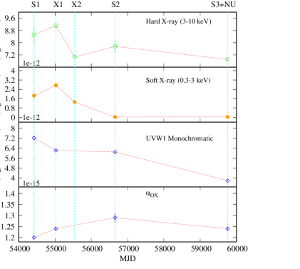
In the previous sections, we presented spectral fit results using several phenomenological and physical models applied to the data of Mrk 50. We observed that in S1 observation, the total X-ray flux (0.3–10 keV) was erg cm-2 s-1, which increased by approximately 1.4 times ( erg cm-2 s-1) in the X1 observation. However, within a year, the flux dropped by a factor of approximately 1.5 in the X2 observation. The calculated flux in X2 observation was erg cm-2 s-1. After that, the total X-ray flux decreased to erg cm-2 s-1 in the most recent observation S3+NU, which is approximately 2.5 times less than the flux in the X1 observation. From Table 7, it is evident that both the hard X-ray and UV monochromatic flux varied significantly between the observations. The UV monochromatic flux (UVW1) was erg cm-2 s-1 Å-1in S1 and then declines to erg cm-2 s-1 Å-1in S3+NU observation.

The variation in the X-ray flux over time may arise due to changes in the strength of Comptonization inside the Compton cloud. It is also believed that these variations may be attributed to changes in the UV photon flux. Simultaneous UV and X-ray observations allow us to probe these types of spectral variability. For this purpose, a hypothetical power-law between 2500 Å and 2 keV, known as (Tananbaum et al., 1979), is estimated from the simultaneous UV and X-ray observations. The parameter is defined as =. We used the UVW1 band to compute because it has the closest effective wavelength to 2500 Å . The observed values remain nearly constant at across all observations, suggesting that the X-ray and UV photons vary in a similar manner. The steeper value of this parameter indicates that the X-ray emission is dimmed more than the UV emission. This phenomenon is commonly observed in the case of most AGNs (Strateva et al., 2005). According to Gallo (2006), steep is often accompanied by X-ray spectral complexity such as enhanced blurred reflection. Due to relativistic effects, most of the emission from the primary power-law component bends towards the black hole, preventing it from reaching the observer (Miniutti & Fabian, 2004; Pal et al., 2018). In comparison, the UV emission (produced by the colder accretion disc) remains relatively unchanged. A relatively weaker X-ray and constant UV emission makes steep.
During the spectral fitting, the softest spectrum is observed in the S1 observation with the primary continuum power-law slope of (see Table 3). The normalized accretion rate for this observation is estimated to be (see Table 5), the highest among all observations. As the accretion rate is high, the emission from the disk is significant, indicating an increased supply of seed photons. As a result, a soft spectrum is observed for this observation. With the increase in the supply of seed photons, more photons interact within the Compton cloud, increasing the luminosity of the primary continuum. For this observation, the luminosity of the primary continuum is found to be , the highest among all the observations used in the present work. Due to the high accretion rate, the UV flux also increased. We observed the highest UV fluxes of , and erg cm-2 s-1 Å-1(see Table 7) for the wavelength 1928 Å(UVW2), 2310 Å(UVM2) and 2930 Å(UVW1), respectively, for this observation. As both UV and X-ray fluxes increased, we found the UV to X-ray slope, (see Table 7), which is comparable with other observations.
From the spectral analysis, a marginal presence of soft excess was observed in the S1 observation (see the first panel of Figure 2). Initially, this excess component was characterized by a power-law with a photon index () of (see Table 3). Later, it was described by a multicolour disk blackbody () with inner disk temperature () at keV (see Table 4). If the soft excess is attributed to the Comptonization of seed photons from a warm corona, the optical depth of the corona is estimated to be , with a dimension of (see Table 5). On the other hand, if the soft excess results from reflection processes, the reflection coefficient is determined to be with a photon index (see Table 6).
After a two-year gap from the S1 observation, the next X-ray observation was conducted with XMM-Newton in 2009 (X1). The X-ray continuum became hard during this observation with a photon index of . The luminosity of the primary continuum marginally decreased from to (see Table 3) within two years. A decrease in luminosity suggests a decrease in the accretion rate, estimated to be , lower than the previous observation (see Table 5).
With decreasing accretion rate, the number of seed photons decreases. The decreasing number of seed photons is unable to cool the warm corona efficiently due to less scattering and is most likely responsible for the expansion of the warm corona. In this work, we found an increase in the value of and a decrease in the accretion rate as found in other AGNs, e.g., Mrk 1018 (Noda & Done, 2018) and NGC 1566 (Tripathi & Dewangan, 2022). This decrease in accretion rate also results in a reduction in UV flux, measured at and erg cm-2 s-1 Å-1for wavelengths 2310Å and 2930Å, respectively (see Table 7). Although both UV and X-ray fluxes decrease, the slope remains constant (, as noted in Table 7).
From spectral analysis, a strong soft excess is observed in this observation (second panel of Figure 2). This soft excess is characterized by a power-law with photon index and luminosity of and , respectively. This represents the highest soft excess luminosity among all observations from 2007 (S1) to 2022 (S3+NU). The optical depth and coronal radius are also found to maximum ( and ; see Table 5) during this observation. This higher optical depth and larger corona generate more soft X-ray photons, resulting in the strong presence of soft excess. The reflection model suggests a stronger reflection during this observation, with the inner disk deviating from Newtonian geometry (inner emissivity index ), producing a steeper power-law with photon index .
During the X2 observation, the observed soft excess is relatively low, irrespective of the similar nature of the primary power-law continuum. The slope of the primary continuum and corresponding luminosity during this observation are and , respectively, consistent with the X1 observation. The soft excess luminosity declined from during X1 observation, to during X2 observation. This decrease in the soft excess can be explained by the warm Comptonization model. Using this model, we found that the optical depth decreased from to , while the size of the warm corona contracted from to . A smaller size of warm corona with a relatively small optical depth produces less number of X-ray photons in soft X-ray band. Therefore, the observed decrease in the soft excess luminosity during observation X2, compared to that during X1, is due to the decrease in the size and optical depth of the warm corona. We also attempted to describe the soft excess using the reflection model. In this model, we also noticed that the value of the reflection coefficient decreased from to . As a result, fewer photons were effectively reflected to produce excess emission below 2 keV.
During the S2 observation, we encountered the hardest spectrum of Mrk 50 with an index and corresponding luminosity of the primary continuum as , and , respectively. From the physical model fitting, the accretion rate is estimated to be (), the lowest among all the observations. We also noticed that the amount of soft excess is remarkably reduced and falls below the detection limit. This is possibly due to the low exposure time of this observation. In this case, the slope of the power-law representing the soft excess is comparable with the slope of the primary continuum. Although the effective size of the warm corona was not reduced at the time of observation, the optical depth decreased from (X2 observation) to (S1 observation). Consequently, very few excess photons are produced in the soft X-ray range. Therefore, most of the photons observed in the soft X-ray regime are from the primary continuum through the process of Comptonization in the hot corona. From the reflection model perspective, we found that the reflection coefficient is , much lower than other observations. As a result, fewer reflected photons are produced to contribute towards the excess emission in the soft X-ray domain. Additionally, we found that the dimensions of the Compton cloud or corona are of the same order as calculated from different models for this observation.
The latest observation in the X-ray domain was conducted with the Swift and NuSTAR observatories in 2022 (S3+NU). Using these observations, we obtained a broadband spectrum of Mrk 50 starting from UV to hard X-ray range. We noticed that while extending the primary continuum up to 100 keV, no deviation was seen in the spectra, indicating the absence of a reflection hump above 10 keV. During this observation, the primary continuum luminosity , lowest among all the observations, with . The normalized accretion rate increased from (S2 observation) to during this observation. Since the soft excess component is below the detection limit, determining parameters associated with the warm corona is challenging. However, spectral analysis indicates an optical depth of and a transitional radius of for this observation. Therefore, the observed broadband spectrum (from UV to hard X-ray range) is dominated by the primary continuum with power-law fraction . From the reflection model perspective, the whole disk followed the Newtonian geometry with a negligible amount of reflection (). Thus, photon contribution in the soft X-ray band is nearly negligible. Consequently, a single power-law model is sufficient to fit the broadband spectrum from 1 eV to 100 keV.
For the overall picture, we observed that the slope of the primary continuum varied from to . However, the primary continuum luminosity remained nearly constant, with an average value of . In contrast, for the soft excess component (below 3 keV), we found that both the power-law index() and luminosity () varied within the ranges of to and to , respectively. We explored the possible physical reasons for this spectral variability and found that the variation in the primary continuum can be explained in terms of accretion dynamics. Depending on the accretion rates and the efficiency of the Compton cloud, the slope of different spectral components and the corresponding luminosity change. The long-term variations of a few spectral parameters are presented in Figure 7.

| Spectral | Flux | Flux | Flux | Flux | Flux |
|---|---|---|---|---|---|
| Component | S1 | X1 | X2 | S2 | S3+NU |
| Soft X-ray Excess1 ( | |||||
| Hard X-ray Flux ( | |||||
| Total X-ray Flux () | |||||
| UVW2 () | – | – | |||
| UVM2 () | – | ||||
| UVW1 () | – | ||||
| – |
1The X-ray fluxes are in the unit of erg cm-2 s-1.
2The UV monochromatic fluxes are measured from Swift UVOT and XMM-Newton OM instruments. The fluxes are in
the unit of erg cm-2 s-1 Å-1.
4.3 Relation between different spectral parameters
In the previous section, we explained the observed spectral variabilities in Mrk 50 using various spectral parameters derived from different model fittings (see Section 3.2). Although all of the model parameters contribute to the overall spectral variability, they are not entirely independent of each other. In this subsection, we examine the correlations between different spectral parameters. We calculated the Correlation Coefficient131313https://www.statskingdom.com/correlation-calculator.html (CC) to calculate the degree of correlation between the parameters. The correlations between some selected parameters are shown in Figure 10. This limited number of observations (five) in a period of 15 years makes it challenging to draw definitive physical conclusions about the correlations between different parameters. However, we discuss the observed trends in the correlation between different parameters on this 15-year timescale. Based on these correlation studies, we infer the nature of the source and understand the overall spectral properties of Mrk 50.
We began our spectral analysis by parameterizing the observed spectra using a power-law model, calculating the spectral slopes and luminosities and/or fluxes of different spectral components, including the soft excess and the primary continuum. We observed hints of correlations between luminosities and fluxes in the hard and soft X-ray regions, with correlation coefficients (CC) of 0.66 () and 0.78 (), respectively, as shown in Figure 10 panels (a) and (b). Similar correlations have been observed in other AGNs, such as IC 4329A (Tripathi et al., 2021), PKS 0558-504 (Gliozzi et al., 2013), NGC 7469 (Nandra & Papadakis, 2001) and have been interpreted in terms of thermal Componization of soft photons in the hot corona. As the number of soft photons increases, the number of scattering in the hot corona also increases, leading to an enhancement in the Comptonized X-ray flux. This common feature is also observed in ‘bare’ AGNs (Nandi et al., 2021, 2023).
Additionally, we found that the UV flux correlates with both soft and hard X-ray fluxes, with CC=0.61 () for soft X-ray vs. UV, and CC=0.79 () for hard X-ray vs. UV. These correlations indicate a relationship between the disk and the hot corona, and a link between the disk and the medium producing the soft excess. Furthermore, we observed a correlation trend between the spectral slope of the primary continuum () and the normalized accretion rate , with a CC of 0.89 (). The - correlation indicates the connection between the accretion disk and the X-ray corona. The physics behind this correlation is not clear. One possible explanation is that a higher accretion rate increases the supply of soft photons; an increase in the supply of soft photons can produce more hard photons by interacting with the Compton cloud. Consequently, the power-law index steepens, leading to the observed correlation between and (Fabian et al., 2015; Ricci et al., 2018; Vasudevan & Fabian, 2007; Layek et al., 2024).
Next, we applied physical models to the observed spectra to explain the nature and origin of the different spectral components. We found a hint of a correlation between the reflection coefficient () and the slope of the soft excess component (). Since the model fits the X-ray spectra well, this correlation may suggest a link between and in the X-ray band, implying that the soft excess component may be associated with the reflection phenomena. We also explored the correlation between the UV to X-ray index, , and various spectral parameters, finding that is anti-correlated with , with (-value=0.11). Since remains nearly constant at 1.24 across our observations, and the values from different observations fall within the range of uncertainties, it is challenging to comment on this anti-correlation conclusively. The dependence of with suggests that the disc/corona relative intensity also depends on the accretion rate (Fanali et al., 2013).
In this study, we explored correlations between various parameters and found hints of correlations between the spectral parameters. These correlations can be explained from a physical perspective. However, it is important to note that the -values associated with these correlations are greater than 0.05, indicating that the correlations may not be statistically significant at the 5% level. This suggests that the observed relationships could potentially be due to random variability. Further investigation or a larger sample size may be needed to draw more accurate conclusions.
4.4 Soft Excess
An enhancement of flux in the soft X-ray range (below keV) over the primary power-law continuum is commonly observed in most of the Seyfert 1 AGNs. This excess in the low energy range is known as soft excess. Our spectral analysis revealed the presence of a prominent soft excess below 2 keV in Mrk 50. However, this soft excess component is found to change over time. From the flux calculations, we observed significant variability in soft excess flux between observations of Mrk 50 (see Table 7). This appearance and disappearance of the soft excess component intrigued us to explore its origin. Although the origin of this excess emission in the soft X-ray domain is a long-standing and unsolved puzzle in AGN studies, we attempted to unravel this mystery using various models discussed in Section 3.3.
4.4.1 Strength of soft excess
Among all the observations used in the present work, the observed soft excess component is the strongest in the 2009 observation (X1). During this observation, the Fe line and the Compton hump are also not detected in the spectrum. Spectral modelling in such cases is often challenging due to the limited number of spectral components. Besides this, the UV/X-ray combined spectra were not explored. Therefore, we initially characterized the soft excess component with a simple power-law over the primary continuum.
Although the initial characterization of the soft excess component using a power-law model provided valuable insights into the temporal variation of this component, the variation of its strength relative to the primary continuum still needs to be explored. We employed a multicoloured blackbody model Diskbb (Mitsuda et al., 1984), replacing the power-law component for the soft excess. We fitted all observed spectra with this model and found that the blackbody temperature varies within a narrow range from to keV. The soft excess is modeled as a blackbody, and its strength () is defined as the ratio of the luminosity in the blackbody component to the luminosity in the power-law between 3 and 10 keV, as described by (Vasudevan et al., 2013). The parameter is used to investigate if there is a positive link between the strength of the soft excess and reflection. Vasudevan et al. (2013) and Boissay et al. (2016) used this parameter to investigate whether reflection is the cause of the soft excess.
In the first three observations (S1, X1, and X2), the presence of soft excess is clearly detected, whereas it is barely detected in the spectra of the observations in 2013 (S2) and 2022 (S3+NU). We examine the correlation between the strength of soft excess () and power-law photon index (), power-law luminosity (), and reflection strength () (see Figure 9). Although it is challenging to determine whether a correlation or anti-correlation exists between these parameters due to the limited number of observations, we observed a hint of a correlation between and . Such a correlation has previously been observed in a larger sample of AGNs (Boissay et al., 2016; Vasudevan et al., 2013).
4.4.2 Origin of soft excess
The soft X-ray excess observed in AGN was initially represented as a high-frequency tail of the disk emission (Singh et al., 1985; Pounds et al., 1986; Leighly, 1999a; Magdziarz et al., 1998; Leighly, 1999b). In many AGNs, this soft excess could be fitted by a blackbody model with a best-fit temperature of 0.1– 0.2 keV (Walter & Fink, 1993; Czerny et al., 2003; Jana et al., 2021); however, this temperature is significantly higher than the maximum temperatures expected in AGN accretion disk. This temperature is nearly independent of the accretion rate (see Table 5). As a result, the inner disk is unlikely to be the source of the soft excess emission. Recent studies suggest that the soft excess in Seyfert 1s can be successfully described by both the intrinsic thermal Comptonization of disk photons (Done et al., 2012; Kubota & Done, 2018; Petrucci et al., 2018, 2020) and relativistic reflections from an ionized accretion disk (Ehler et al., 2018; García et al., 2019; Ghosh & Laha, 2020; Yu et al., 2023). So, to investigate the possible origin of the soft excess, we explored two physically motivated scenarios: the warm Comptonized disk emission model (Optxagnf) and the blurred reflection model (Relxillcp).
The Optxagnf model has three distinct emission components: the UV bump from the disk, the soft excess component from the warm corona, and the hard X-ray power-law from the hot corona, assuming that all are powered by gravitational energy released through the process of accretion (Done et al., 2012). The model can potentially explain the origin and variation of the soft excess. The best-fit result using this model is presented in Section 3.4.1. The results indicate that more than 80% () of the power-law is generated from the hot corona via the process of inverse Comptonization. Only 10–20% of the total photons in the spectrum are involved in generating the soft excess component. This result is also cross-verified by the flux calculations in Table 7. In Optxagnf model, the soft excess emission is produced due to the thermal Comptonization of the disk optical-UV photons by a warm (0.1–0.2 keV) optically thick (10–20) corona surrounding the inner region of the disk. For AGN soft excess, the soft X-ray emitting plasma temperature is degenerate with the optical depth () (Turner et al., 2018). In the case of Mrk 50, we also found that the warm corona temperature () and optical depth are degenerate (see Figure 5). At a particular source luminosity or spectral state, an increase in in the model is compensated by a decrease in in the fit and vice versa. From spectral analysis, we found that best-fit values of the temperature of the warm corona vary between keV to keV. The strength of the soft excess varies between 0.22–0.05. Hence, the variation in the strength of the soft excess can be explained by the change in the size of the warm corona () and its Comptonization efficiency. During 2009 observation (X1), we found that the warm corona extends up to the maximum value with an optical depth and corresponding soft X-ray flux maximized in this observation period. Before (2007) and after (2010) this observation, the values of these parameters decrease. Consequently, the strength of the soft excess drops, and the flux is reduced. However, we could not determine the exact size (), electron temperature () and optical depth () of the Comptonizing corona when the soft excess is absent.
The blurred reflection model can also explain the origin and variation of the soft excess in Mrk 50. We begin our analysis using the Relxillcp model. However, the absence of key reflection features, such as a prominent Fe line and reflection hump above 10 keV, along with deviations in the UV band, indicated that pure reflection can not explain the observed spectra of Mrk 50 across the UV to X-ray range. The deviations in the UV bands required an additional power-law component in the spectral fitting. The variation in the soft excess strength can be explained using the boundary of the inner accretion disk () and the reflection efficiency (). The inner disk in Mrk 50 was found to be extended up to with maximum reflection efficiency of during the 2009 observation (X1), where the strength of the soft excess was maximum. The break radius (boundary of the inner disk) and the reflection efficiency decreased as the strength of the soft excess decreased before (S1) and after (X2, S2, and S3+NU) this observation (see Table 5).
When we consider only X-ray data, both the reflection and warm corona scenarios could explain the origin of the soft excess in Mrk 50. Both models are statistically acceptable while fitting data beyond 0.3 keV. However, the origin of the soft excess can be further investigated through timing analysis. The cross-correlation function (CCF) analysis is another approach to distinguish the physical mechanisms behind the origin of soft excess in AGNs. This is a model-independent method to study the correlations and delays between the soft and hard X-ray bands. In the relativistic blurred reflection model, the soft excess is known to have originated due to the ionized reflection of hard X-ray photons from the hot corona in the inner region of the accretion disk. Therefore, one can expect a short delay (30 seconds) between the hard and soft X-ray emission, observed in narrow-line Seyfert 1 AGNs (Fabian et al., 2009; Emmanoulopoulos et al., 2011). On the other hand, a longer delay could be produced by Comptonization. In the context of the Optxagnf model, the soft excess emission is attributed to the disk, with the inner region acting as an optically thick Comptonizing corona (Done et al., 2012). An extensive study on the soft X-ray time lag reports that the lags originate from the inner part of the accretion disk, which is highly dependent on the mass of the central object (De Marco et al., 2013). However, our timing study shows no correlation between the soft and hard bands (see Figure 1). This suggests that both the Comptonization and reflection processes contribute towards the origin of soft excess in Mrk 50 as in case of AGN, ESO 141-G055 (Ghosh & Laha, 2020). Based on spectral analysis, we tentatively conclude that the warm Comptonization model is a favorable explanation for the soft excess in Mrk 50. However, we cannot rule out the relativistic reflection model if we consider only X-ray data beyond 0.3 keV in the spectral fitting. Detailed investigation on the origin of soft excess in Mrk 50 using different models requires high-quality simultaneous observations by XMM-Newton and NuSTAR, as well as future X-ray missions like Athena, which is beyond the scope of this work.


5 Conclusions
For the first time, we presented a temporal and spectral study of the Seyfert 1 AGN Mrk 50 based on long-term observations over 15 years (2007–2022). Our key findings are the following.
-
1.
Based on our spectral analysis, we notice that the observed spectra are almost unaffected by intrinsic hydrogen column densities, indicating that Mrk 50 has a ‘bare’ nucleus at its centre.
-
2.
From the year (2007–2022) long observations of Mrk 50, we observe that the source moved from a comparatively soft state in 2007 to a comparatively hard state in 2013, and then back to a soft state in 2022.
-
3.
The observed variation in the spectral slope () can be attributed to the dynamics of the accretion flow surrounding the central supermassive black hole and the characteristics of the Compton cloud. Our analysis reveals that the normalized accretion rate decreases from to , while changes from to . The accretion rate then increases to , corresponding to . During these spectral transitions of Mrk 50, the warm corona, as described by the warm Comptonization model, and the inner disk boundary, as described by the blurred reflection model, change accordingly.
-
4.
During our spectral analysis, the soft excess component varies throughout the observational period. In the 2009 observation, we found the strongest presence of this component in the observed spectrum. However, before and after 2009, this component gradually faded. The appearance and disappearance of the soft excess component can be explained by the dynamics of accretion and the properties of the Compton cloud.
-
5.
The warm Comptonization model and the blurred reflection model are used to explain the spectral appearance and disappearance of the soft excess component in Mrk 50. Both models provide a satisfactory explanation for the variation in the soft excess. According to these models, the inner part of the disk plays a crucial role in generating the soft excess component, and variations in this part of the disk result in changes in the intensity of the soft excess. The soft excess appears when the warm corona is present. On the other hand, according to the reflection model, the intensity of the soft excess increases when the amount of reflection is high.
-
6.
From the temporal properties of Mrk 50, we found that the source was variable during the 2007 observation. After that, Mrk 50 became non-variable throughout the observational period from 2009 to 2022. Additionally, our cross-correlation study found no correlation between the soft and hard bands. This may indicate that both the Comptonization and reflection processes contribute towards the origin of soft excess in Mrk 50.
Acknowledgements
We sincerely thank the anonymous referee for his/her insightful comments and constructive suggestions that helped us to improve the manuscript. The research work at the Physical Research Laboratory, Ahmedabad, is funded by the Department of Space, Government of India. AJ acknowledges support from the FONDECYT Postdoctoral fellowship (3230303). The data and the software used in this work are taken from the High Energy Astrophysics Science Archive Research Center (HEASARC), which is a service of the Astrophysics Science Division at NASA/GSFC and the High Energy Astrophysics Division of the Smithsonian Astrophysical Observatory. This work has made use of data obtained from the NuSTAR mission, a project led by Caltech, funded by NASA and managed by NASA/JPL, and has utilized the NuSTARDAS software package, jointly developed by the ASDC, Italy and Caltech, USA. This work made use of data Swift supplied by the UK Swift Science Data Centre at the University of Leicester. This research has used observations obtained with XMM-Newton, an ESA science mission with instruments and contributions directly funded by ESA Member States and NASA.
References
- Alexander (1997) Alexander, T. 1997, in Astrophysics and Space Science Library, Vol. 218, Astronomical Time Series, ed. D. Maoz, A. Sternberg, & E. M. Leibowitz, 163, doi: 10.1007/978-94-015-8941-3_14
- Alexander (2013) Alexander, T. 2013, arXiv e-prints, arXiv:1302.1508, doi: 10.48550/arXiv.1302.1508
- Antonucci (1993) Antonucci, R. 1993, ARA&A, 31, 473, doi: 10.1146/annurev.aa.31.090193.002353
- Arnaud (1996) Arnaud, K. A. 1996, in Astronomical Society of the Pacific Conference Series, Vol. 101, Astronomical Data Analysis Software and Systems V, ed. G. H. Jacoby & J. Barnes, 17
- Arnaud et al. (1985) Arnaud, K. A., Branduardi-Raymont, G., Culhane, J. L., et al. 1985, MNRAS, 217, 105, doi: 10.1093/mnras/217.1.105
- Barth et al. (2011) Barth, A. J., Pancoast, A., Thorman, S. J., et al. 2011, ApJ, 743, L4, doi: 10.1088/2041-8205/743/1/L4
- Barthelmy et al. (2005) Barthelmy, S. D., Barbier, L. M., Cummings, J. R., et al. 2005, Space Sci. Rev., 120, 143, doi: 10.1007/s11214-005-5096-3
- Bennett et al. (2003) Bennett, C. L., Halpern, M., Hinshaw, G., et al. 2003, ApJS, 148, 1, doi: 10.1086/377253
- Bentz & Katz (2015) Bentz, M. C., & Katz, S. 2015, PASP, 127, 67, doi: 10.1086/679601
- Bianchi et al. (2009) Bianchi, S., Bonilla, N. F., Guainazzi, M., Matt, G., & Ponti, G. 2009, A&A, 501, 915, doi: 10.1051/0004-6361/200911905
- Boissay et al. (2016) Boissay, R., Ricci, C., & Paltani, S. 2016, A&A, 588, A70, doi: 10.1051/0004-6361/201526982
- Burrows et al. (2005) Burrows, D. N., Hill, J. E., Nousek, J. A., et al. 2005, Space Sci. Rev., 120, 165, doi: 10.1007/s11214-005-5097-2
- Cardelli et al. (1989) Cardelli, J. A., Clayton, G. C., & Mathis, J. S. 1989, ApJ, 345, 245, doi: 10.1086/167900
- Chakrabarti & Titarchuk (1995) Chakrabarti, S., & Titarchuk, L. G. 1995, ApJ, 455, 623, doi: 10.1086/176610
- Chalise et al. (2022) Chalise, S., Lohfink, A. M., Chauhan, J., et al. 2022, MNRAS, 517, 4788, doi: 10.1093/mnras/stac2953
- Crummy et al. (2006) Crummy, J., Fabian, A. C., Gallo, L., & Ross, R. R. 2006, MNRAS, 365, 1067, doi: 10.1111/j.1365-2966.2005.09844.x
- Czerny & Elvis (1987) Czerny, B., & Elvis, M. 1987, ApJ, 321, 305, doi: 10.1086/165630
- Czerny et al. (2003) Czerny, B., Nikołajuk, M., Różańska, A., et al. 2003, A&A, 412, 317, doi: 10.1051/0004-6361:20031441
- Dauser et al. (2014) Dauser, T., Garcia, J., Parker, M. L., Fabian, A. C., & Wilms, J. 2014, MNRAS, 444, L100, doi: 10.1093/mnrasl/slu125
- Dauser et al. (2016) Dauser, T., García, J., Walton, D. J., et al. 2016, A&A, 590, A76, doi: 10.1051/0004-6361/201628135
- De Marco et al. (2013) De Marco, B., Ponti, G., Cappi, M., et al. 2013, MNRAS, 431, 2441, doi: 10.1093/mnras/stt339
- den Herder et al. (2001) den Herder, J. W., Brinkman, A. C., Kahn, S. M., et al. 2001, A&A, 365, L7, doi: 10.1051/0004-6361:20000058
- Done et al. (2012) Done, C., Davis, S. W., Jin, C., Blaes, O., & Ward, M. 2012, MNRAS, 420, 1848, doi: 10.1111/j.1365-2966.2011.19779.x
- Done et al. (2007) Done, C., Gierliński, M., & Kubota, A. 2007, A&A Rev., 15, 1, doi: 10.1007/s00159-007-0006-1
- Edelson & Malkan (2012) Edelson, R., & Malkan, M. 2012, ApJ, 751, 52, doi: 10.1088/0004-637X/751/1/52
- Edelson et al. (2002) Edelson, R., Turner, T. J., Pounds, K., et al. 2002, ApJ, 568, 610, doi: 10.1086/323779
- Edelson & Krolik (1988) Edelson, R. A., & Krolik, J. H. 1988, ApJ, 333, 646, doi: 10.1086/166773
- Edelson et al. (1996) Edelson, R. A., Alexander, T., Crenshaw, D. M., et al. 1996, ApJ, 470, 364, doi: 10.1086/177872
- Ehler et al. (2018) Ehler, H. J. S., Gonzalez, A. G., & Gallo, L. C. 2018, MNRAS, 478, 4214, doi: 10.1093/mnras/sty1306
- Emmanoulopoulos et al. (2011) Emmanoulopoulos, D., McHardy, I. M., & Papadakis, I. E. 2011, MNRAS, 416, L94, doi: 10.1111/j.1745-3933.2011.01106.x
- Evans et al. (2009) Evans, P. A., Beardmore, A. P., Page, K. L., et al. 2009, MNRAS, 397, 1177, doi: 10.1111/j.1365-2966.2009.14913.x
- Event Horizon Telescope Collaboration et al. (2019) Event Horizon Telescope Collaboration, Akiyama, K., Alberdi, A., et al. 2019, ApJ, 875, L1, doi: 10.3847/2041-8213/ab0ec7
- Fabian et al. (2002) Fabian, A. C., Ballantyne, D. R., Merloni, A., et al. 2002, MNRAS, 331, L35, doi: 10.1046/j.1365-8711.2002.05419.x
- Fabian et al. (2015) Fabian, A. C., Lohfink, A., Kara, E., et al. 2015, MNRAS, 451, 4375, doi: 10.1093/mnras/stv1218
- Fabian et al. (2009) Fabian, A. C., Zoghbi, A., Ross, R. R., et al. 2009, Nature, 459, 540, doi: 10.1038/nature08007
- Fanali et al. (2013) Fanali, R., Caccianiga, A., Severgnini, P., et al. 2013, MNRAS, 433, 648, doi: 10.1093/mnras/stt757
- Foreman-Mackey (2017) Foreman-Mackey, D. 2017, corner.py: Corner plots, Astrophysics Source Code Library, record ascl:1702.002
- Gallo (2006) Gallo, L. C. 2006, MNRAS, 368, 479, doi: 10.1111/j.1365-2966.2006.10137.x
- García et al. (2013) García, J., Dauser, T., Reynolds, C. S., et al. 2013, ApJ, 768, 146, doi: 10.1088/0004-637X/768/2/146
- García & Kallman (2010) García, J., & Kallman, T. R. 2010, ApJ, 718, 695, doi: 10.1088/0004-637X/718/2/695
- García et al. (2014) García, J., Dauser, T., Lohfink, A., et al. 2014, ApJ, 782, 76, doi: 10.1088/0004-637X/782/2/76
- García et al. (2018) García, J. A., Steiner, J. F., Grinberg, V., et al. 2018, The Astrophysical Journal, 864, 25
- García et al. (2019) García, J. A., Kara, E., Walton, D., et al. 2019, ApJ, 871, 88, doi: 10.3847/1538-4357/aaf739
- Gehrels et al. (2004) Gehrels, N., Chincarini, G., Giommi, P., et al. 2004, ApJ, 611, 1005, doi: 10.1086/422091
- George & Fabian (1991) George, I. M., & Fabian, A. C. 1991, MNRAS, 249, 352, doi: 10.1093/mnras/249.2.352
- Ghosh & Laha (2020) Ghosh, R., & Laha, S. 2020, MNRAS, 497, 4213, doi: 10.1093/mnras/staa2259
- Ghosh et al. (2022) Ghosh, R., Laha, S., Deshmukh, K., et al. 2022, ApJ, 937, 31, doi: 10.3847/1538-4357/ac887e
- Gierliński & Done (2004) Gierliński, M., & Done, C. 2004, MNRAS, 349, L7, doi: 10.1111/j.1365-2966.2004.07687.x
- Gliozzi et al. (2013) Gliozzi, M., Papadakis, I. E., Grupe, D., Brinkmann, W. P., & Räth, C. 2013, MNRAS, 433, 1709, doi: 10.1093/mnras/stt848
- Goodman & Weare (2010) Goodman, J., & Weare, J. 2010, Communications in Applied Mathematics and Computational Science, 5, 65, doi: 10.2140/camcos.2010.5.65
- Haardt & Maraschi (1991) Haardt, F., & Maraschi, L. 1991, ApJ, 380, L51, doi: 10.1086/186171
- Haardt & Maraschi (1993) —. 1993, ApJ, 413, 507, doi: 10.1086/173020
- Halpern (1984) Halpern, J. P. 1984, ApJ, 281, 90, doi: 10.1086/162077
- Harrison et al. (2013) Harrison, F. A., Craig, W. W., Christensen, F. E., et al. 2013, ApJ, 770, 103, doi: 10.1088/0004-637X/770/2/103
- Jana et al. (2021) Jana, A., Kumari, N., Nandi, P., et al. 2021, MNRAS, 507, 687, doi: 10.1093/mnras/stab2155
- Jansen et al. (2001) Jansen, F., Lumb, D., Altieri, B., et al. 2001, A&A, 365, L1, doi: 10.1051/0004-6361:20000036
- Jiang et al. (2018) Jiang, J., Parker, M. L., Fabian, A. C., et al. 2018, MNRAS, 477, 3711, doi: 10.1093/mnras/sty836
- Kormendy & Richstone (1995) Kormendy, J., & Richstone, D. 1995, ARA&A, 33, 581, doi: 10.1146/annurev.aa.33.090195.003053
- Krolik (1999) Krolik, J. H. 1999, Active galactic nuclei : from the central black hole to the galactic environment
- Kubota & Done (2018) Kubota, A., & Done, C. 2018, MNRAS, 480, 1247, doi: 10.1093/mnras/sty1890
- Kumari et al. (2023) Kumari, N., Jana, A., Naik, S., & Nandi, P. 2023, MNRAS, 521, 5440, doi: 10.1093/mnras/stad867
- Laha et al. (2014) Laha, S., Guainazzi, M., Dewangan, G. C., Chakravorty, S., & Kembhavi, A. K. 2014, MNRAS, 441, 2613, doi: 10.1093/mnras/stu669
- Laor (1991) Laor, A. 1991, ApJ, 376, 90, doi: 10.1086/170257
- Layek et al. (2024) Layek, N., Nandi, P., Naik, S., et al. 2024, MNRAS, 528, 5269, doi: 10.1093/mnras/stae299
- Leighly (1999a) Leighly, K. M. 1999a, ApJS, 125, 297, doi: 10.1086/313277
- Leighly (1999b) —. 1999b, ApJS, 125, 317, doi: 10.1086/313287
- Madathil-Pottayil et al. (2024) Madathil-Pottayil, A., Walton, D. J., García, J., et al. 2024, MNRAS, 534, 608, doi: 10.1093/mnras/stae2104
- Magdziarz et al. (1998) Magdziarz, P., Blaes, O. M., Zdziarski, A. A., Johnson, W. N., & Smith, D. A. 1998, MNRAS, 301, 179, doi: 10.1046/j.1365-8711.1998.02015.x
- Mason et al. (2001) Mason, K. O., Breeveld, A., Much, R., et al. 2001, A&A, 365, L36, doi: 10.1051/0004-6361:20000044
- Matt et al. (1991) Matt, G., Perola, G. C., & Piro, L. 1991, A&A, 247, 25
- Matzeu et al. (2020) Matzeu, G. A., Nardini, E., Parker, M. L., et al. 2020, MNRAS, 497, 2352, doi: 10.1093/mnras/staa2076
- Middei et al. (2020) Middei, R., Tombesi, F., Vagnetti, F., et al. 2020, A&A, 635, A18, doi: 10.1051/0004-6361/201936701
- Middleton et al. (2009) Middleton, M., Done, C., Ward, M., Gierliński, M., & Schurch, N. 2009, MNRAS, 394, 250, doi: 10.1111/j.1365-2966.2008.14255.x
- Miniutti & Fabian (2004) Miniutti, G., & Fabian, A. C. 2004, MNRAS, 349, 1435, doi: 10.1111/j.1365-2966.2004.07611.x
- Miniutti et al. (2009) Miniutti, G., Ponti, G., Greene, J. E., et al. 2009, MNRAS, 394, 443, doi: 10.1111/j.1365-2966.2008.14334.x
- Mitsuda et al. (1984) Mitsuda, K., Inoue, H., Koyama, K., et al. 1984, PASJ, 36, 741
- Nandi et al. (2021) Nandi, P., Chatterjee, A., Chakrabarti, S. K., & Dutta, B. G. 2021, MNRAS, 506, 3111, doi: 10.1093/mnras/stab1699
- Nandi et al. (2023) Nandi, P., Chatterjee, A., Jana, A., et al. 2023, ApJS, 269, 15, doi: 10.3847/1538-4365/acf4f9
- Nandi et al. (2024) Nandi, P., Naik, S., Chatterjee, A., et al. 2024, MNRAS, doi: 10.1093/mnras/stae1529
- Nandra et al. (1997) Nandra, K., George, I. M., Mushotzky, R. F., Turner, T. J., & Yaqoob, T. 1997, ApJ, 476, 70, doi: 10.1086/303600
- Nandra & Papadakis (2001) Nandra, K., & Papadakis, I. E. 2001, ApJ, 554, 710, doi: 10.1086/321423
- Narayan & Yi (1994) Narayan, R., & Yi, I. 1994, ApJ, 428, L13, doi: 10.1086/187381
- Netzer (2013) Netzer, H. 2013, The Physics and Evolution of Active Galactic Nuclei
- Noda & Done (2018) Noda, H., & Done, C. 2018, MNRAS, 480, 3898, doi: 10.1093/mnras/sty2032
- Pal et al. (2018) Pal, M., Dewangan, G. C., Kembhavi, A. K., Misra, R., & Naik, S. 2018, MNRAS, 473, 3584, doi: 10.1093/mnras/stx2608
- Pancoast et al. (2012) Pancoast, A., Brewer, B. J., Treu, T., et al. 2012, ApJ, 754, 49, doi: 10.1088/0004-637X/754/1/49
- Pastoriza et al. (1991) Pastoriza, M. G., Bica, E., Bonatto, C., Mediavilla, E., & Perez, E. 1991, AJ, 102, 1696, doi: 10.1086/115989
- Peterson et al. (2004) Peterson, B. M., Ferrarese, L., Gilbert, K. M., et al. 2004, ApJ, 613, 682, doi: 10.1086/423269
- Petrucci et al. (2018) Petrucci, P. O., Ursini, F., De Rosa, A., et al. 2018, A&A, 611, A59, doi: 10.1051/0004-6361/201731580
- Petrucci et al. (2020) Petrucci, P. O., Gronkiewicz, D., Rozanska, A., et al. 2020, A&A, 634, A85, doi: 10.1051/0004-6361/201937011
- Piconcelli et al. (2005) Piconcelli, E., Jimenez-Bailón, E., Guainazzi, M., et al. 2005, A&A, 432, 15, doi: 10.1051/0004-6361:20041621
- Porquet et al. (2024) Porquet, D., Reeves, J. N., Hagen, S., et al. 2024, A&A, 689, A336, doi: 10.1051/0004-6361/202449708
- Porquet et al. (2004) Porquet, D., Reeves, J. N., O’Brien, P., & Brinkmann, W. 2004, A&A, 422, 85, doi: 10.1051/0004-6361:20047108
- Pounds et al. (1986) Pounds, K. A., Warwick, R. S., Culhane, J. L., & de Korte, P. A. J. 1986, MNRAS, 218, 685, doi: 10.1093/mnras/218.4.685
- Rees (1984) Rees, M. J. 1984, ARA&A, 22, 471, doi: 10.1146/annurev.aa.22.090184.002351
- Ricci et al. (2018) Ricci, C., Ho, L. C., Fabian, A. C., et al. 2018, MNRAS, 480, 1819, doi: 10.1093/mnras/sty1879
- Rodríguez-Pascual et al. (1997) Rodríguez-Pascual, P. M., Alloin, D., Clavel, J., et al. 1997, ApJS, 110, 9, doi: 10.1086/312996
- Roming et al. (2005) Roming, P. W. A., Kennedy, T. E., Mason, K. O., et al. 2005, Space Sci. Rev., 120, 95, doi: 10.1007/s11214-005-5095-4
- Ross & Fabian (1993) Ross, R. R., & Fabian, A. C. 1993, MNRAS, 261, 74, doi: 10.1093/mnras/261.1.74
- Ross & Fabian (2005) —. 2005, MNRAS, 358, 211, doi: 10.1111/j.1365-2966.2005.08797.x
- Schlafly & Finkbeiner (2011) Schlafly, E. F., & Finkbeiner, D. P. 2011, ApJ, 737, 103, doi: 10.1088/0004-637X/737/2/103
- Shakura & Sunyaev (1973) Shakura, N. I., & Sunyaev, R. A. 1973, A&A, 24, 337
- Singh et al. (1985) Singh, K. P., Garmire, G. P., & Nousek, J. 1985, ApJ, 297, 633, doi: 10.1086/163560
- Strateva et al. (2005) Strateva, I. V., Brandt, W. N., Schneider, D. P., Vanden Berk, D. G., & Vignali, C. 2005, AJ, 130, 387, doi: 10.1086/431247
- Strüder et al. (2001) Strüder, L., Briel, U., Dennerl, K., et al. 2001, A&A, 365, L18, doi: 10.1051/0004-6361:20000066
- Sun & Malkan (1989) Sun, W.-H., & Malkan, M. A. 1989, ApJ, 346, 68, doi: 10.1086/167986
- Sunyaev & Titarchuk (1980) Sunyaev, R. A., & Titarchuk, L. G. 1980, A&A, 86, 121
- Tananbaum et al. (1979) Tananbaum, H., Avni, Y., Branduardi, G., et al. 1979, ApJ, 234, L9, doi: 10.1086/183100
- Tripathi & Dewangan (2022) Tripathi, P., & Dewangan, G. C. 2022, ApJ, 925, 101, doi: 10.3847/1538-4357/ac3a6e
- Tripathi et al. (2021) Tripathi, P., Dewangan, G. C., Papadakis, I. E., & Singh, K. P. 2021, ApJ, 915, 25, doi: 10.3847/1538-4357/abfe70
- Tripathi et al. (2019) Tripathi, S., Waddell, S. G. H., Gallo, L. C., Welsh, W. F., & Chiang, C. Y. 2019, MNRAS, 488, 4831, doi: 10.1093/mnras/stz1988
- Turner et al. (2001) Turner, M. J. L., Abbey, A., Arnaud, M., et al. 2001, A&A, 365, L27, doi: 10.1051/0004-6361:20000087
- Turner & Pounds (1989) Turner, T. J., & Pounds, K. A. 1989, MNRAS, 240, 833, doi: 10.1093/mnras/240.4.833
- Turner et al. (2018) Turner, T. J., Reeves, J. N., Braito, V., & Costa, M. 2018, MNRAS, 476, 1258, doi: 10.1093/mnras/sty318
- Ursini et al. (2020) Ursini, F., Petrucci, P. O., Bianchi, S., et al. 2020, A&A, 634, A92, doi: 10.1051/0004-6361/201936486
- Vasudevan et al. (2013) Vasudevan, R. V., Brandt, W. N., Mushotzky, R. F., et al. 2013, ApJ, 763, 111, doi: 10.1088/0004-637X/763/2/111
- Vasudevan & Fabian (2007) Vasudevan, R. V., & Fabian, A. C. 2007, MNRAS, 381, 1235, doi: 10.1111/j.1365-2966.2007.12328.x
- Vaughan et al. (2003) Vaughan, S., Edelson, R., Warwick, R. S., & Uttley, P. 2003, MNRAS, 345, 1271, doi: 10.1046/j.1365-2966.2003.07042.x
- Vaughan et al. (2004) Vaughan, S., Fabian, A. C., Ballantyne, D. R., et al. 2004, MNRAS, 351, 193, doi: 10.1111/j.1365-2966.2004.07769.x
- Waddell et al. (2019) Waddell, S. G. H., Gallo, L. C., Gonzalez, A. G., Tripathi, S., & Zoghbi, A. 2019, MNRAS, 489, 5398, doi: 10.1093/mnras/stz2518
- Walter & Fink (1993) Walter, R., & Fink, H. H. 1993, Astronomy and Astrophysics, Vol. 274, NO. 1/JUL (I), P. 105, 1993, 274, 105
- Walton et al. (2013) Walton, D. J., Nardini, E., Fabian, A. C., Gallo, L. C., & Reis, R. C. 2013, MNRAS, 428, 2901, doi: 10.1093/mnras/sts227
- Walton et al. (2010) Walton, D. J., Reis, R. C., & Fabian, A. C. 2010, MNRAS, 408, 601, doi: 10.1111/j.1365-2966.2010.17148.x
- Wilms et al. (2000) Wilms, J., Allen, A., & McCray, R. 2000, ApJ, 542, 914, doi: 10.1086/317016
- Xu et al. (2021) Xu, Y., García, J. A., Walton, D. J., et al. 2021, ApJ, 913, 13, doi: 10.3847/1538-4357/abf430
- Yu et al. (2023) Yu, Z., Jiang, J., Bambi, C., et al. 2023, MNRAS, 522, 5456, doi: 10.1093/mnras/stad1327
- Zdziarski et al. (1996) Zdziarski, A. A., Johnson, W. N., & Magdziarz, P. 1996, MNRAS, 283, 193, doi: 10.1093/mnras/283.1.193
- Życki et al. (1999) Życki, P. T., Done, C., & Smith, D. A. 1999, Monthly Notices of the Royal Astronomical Society, 309, 561, doi: 10.1046/j.1365-8711.1999.02885.x
| Model | ID | ||||||||
|---|---|---|---|---|---|---|---|---|---|
| X1 | – | – | 1(f) | – | – | ||||
| X2 | – | – | – | 1(f) | – | – | |||
| S3+NU | 1(f) | – | – | – | – | ||||
| Model | ID | ||||||||
| X1 | – | – | 1(f) | – | – | ||||
| X2 | – | – | – | 1(f) | – | – | |||
| S3+NU | 1(f) | – | – | – | – | ||||
| Model | ID | ||||||||
| X1 | – | – | 1(f) | – | – | ||||
| X2 | – | – | – | 1(f) | – | – | |||
| S3+NU | 1(f) | – | – | – | – | ||||
| Model | ID | ||||||||
| X1 | – | – | 1(f) | – | – | ||||
| X2 | – | – | – | 1(f) | – | – | |||
| S3+NU | 1(f) | – | – | – | – |
f: indicates a frozen parameter.
