A Lower Bound on Observability for Target Tracking with Range Sensors and its Application to Sensor Assignment
Abstract
We study two sensor assignment problems for multi-target tracking with the goal of improving the observability of the underlying estimator. In the restricted version of the problem, we focus on assigning unique pairs of sensors to each target. We present a –approximation algorithm for this problem. We use the inverse of the condition number as the value function. If the target’s motion model is not known, the inverse cannot be computed exactly. Instead, we present a lower bound for range-only sensing.
In the general version, the sensors must form teams to track individual targets. We do not force any specific constraints on the size of each team, instead assume that the value function is monotonically increasing and is submodular. A greedy algorithm that yields a –approximation. However, we show that the inverse of the condition number is neither monotone nor submodular. Instead, we present other measures that are monotone and submodular. In addition to theoretical results, we evaluate our results empirically through simulations.
I Introduction
State estimation is a fundamental problem in sensorics and finds many applications such as localization, mapping, and target tracking [1, 2]. The estimator performance can be improved by exploiting the observability of the underlying system [3, 4, 5, 6]. We study selecting sensors to improve the observability in tracking a potentially mobile target.
Observability is a basic concept in control theory and has been widely applied in robotics. Observability for range-only beacon sensors, in particular, has been closely studied for underwater navigation. Gadre and Stilwell [3] analyzed the local and global observability [7] for the localization of an Autonomous Underwater Vehicle by an acoustic beacon. The problems of single vehicle localization and multi-vehicle relative localization are studied in [5] using an observability criterion introduced in [8]. In these works, it is the sensors that are moving. Consequently, the sensors know their control vectors and can thus, compute the observability matrix and its measures. In target tracking with fixed or mobile sensors, however, the control inputs for the targets are unknown. In recent work, Williams and Sukhatme [6] studied a multi-sensor localization and target tracking problem where they showed how to leverage graph rigidity to improve the observability for sensor team localization and robust target tracking.
While others have studied similar problems in the past [6, 5], we focus uniquely on the case when the control inputs for the target are not known to the sensors. Consequently, we cannot compute the observability matrix of the resulting system. Our first contribution is to present a novel lower bound on the observability for the case of unknown target motion tracked by range-only sensors. Specifically, we show how to lower bound the condition number [8] of the partially known observability matrix using only the known part (Section III).
We then study two sensor assignment problems. In the first problem, the goal is to assign unique pairs of sensors to a target. Our second contribution is a greedy assignment algorithm for this problem. We prove that the greedy algorithm achieves a –approximation of the optimal solution. We show that the greedy algorithm performs much better than in practice (Section V-C). Since the optimal solution cannot be computed, in order to compare the greedy approach we also consider a relaxed version of the assignment problem which gives an upper bound for the optimal.
We then study a general assignment problem where a set of sensors are to be assigned to a specific target. There are no restrictions on the number of targets assigned to a specific sensor. Instead, we let the algorithm decide the optimal configuration of sensor teams assigned to each target. If the weight function is submodular and monotone111We use “monotone” and “monotone increasing” interchangeably., a greedy algorithm gives a –approximation [9]. However, our third contribution is to prove that the lower bound of the inverse of the condition number is neither submodular nor monotone. Instead, we use other observability measures such as the trace, log determinant and rank of symmetric observability matrix, and the trace of inverse symmetric observability matrix and show them to be submodular and monotone. We evaluate this algorithm through simulations where we find that sensors are assigned to targets almost uniformly (Section V-D).
II Problem Formulation for sensor assignment
We consider a scenario where there are sensors and targets in the environment. Our goal is to assign sensors to track the target. We use the notation to represent the set of sensors assigned to target . Similarly, let give the set of targets assigned to sensor . We also use to give the sensor assigned to . We order the assigned sensors by using their IDs such that . Let , and be some measure of the observability of tracking with and , and with a set of sensor(s) , respectively.
We study the following sensor assignment problems. We start with the problem of assigning pairs of sensors to each target.222Theorems 2 and 3 show that at least two sensors are necessary when is the inverse condition number of the observability matrix.
Problem 1 (Unique Pair Assignment).
Given a set of sensor positions, and a set of target estimates at time , , find an assignment of unique pairs of sensors to targets:
| (1) |
with the added constraint each sensor is assigned to at most one target. That is, for all we have , assuming .
We then study the general version of the problem where each target can be tracked by more than two sensors. That is, the sensors form teams of varying sizes to track individual targets. Sensors within a team can share measurements so as to better track the targets. We constrain each sensor to be assigned to only one target, that is, communicate with only one team. This is motivated by scenarios where sensing multiple targets can be time consuming (as is the case with radio sensors [10]) or communicating multiple measurements can be time and energy consuming.
Problem 2 (General Assignment).
Given a set of sensor positions, and a set of target estimates at time , , find an assignment of sets of sensors to targets:
| (2) |
with the added constraint each sensor is assigned to at most one target.
We present a –approximation to solve Problem 1 for any . Problem 2 is the more general assignment problem which is difficult to solve for arbitrary . However, for the specific class of submodular functions, there exists a –approximation by a greedy algorithm [9]. Submodularity captures the notion of diminishing returns, i.e., the marginal gain of assigning an additional sensor diminishes as more and more sensors are assigned to track the same target.
A typical measure of observability is the condition number of the observability matrix. When the target is moving, the condition number of the observability matrix cannot be computed, since the control input for the target is unknown to the sensors. We find a lower bound on the inverse of the condition number of the observability matrix. We use this lower bound as our measure, i.e., , to find the assignments in Problem 1. However, we show that this measure is not submodular (in fact, not even monotone increasing). Instead, we can use a number of other measures (e.g., the trace of symmetric observability matrix, the trace of inverse symmetric observability matrix, log determinant and rank of the symmetric observability matrix) which we know to be submodular and monotone increasing (Theorem 8). We start by how to bound the inverse of condition number.
III Bounding the Observability
Consider a mobile target whose position is denoted by . Suppose there are stationary sensors that can measure the distance333We use the square of the distance/range for mathematical convenience. to the target. We have:
| (3) |
where gives the 2D position of the target, and defines its control input, which is unknown. We assume an upper bound on the control input, given by . defines the range-only measurement from each sensor whose position is given by . For simplicity, we also assume that the target does not collide with any sensor, i.e., and no two sensors are deployed at the same position.
We analyze the weak local observability matrix, , of this multi-sensor target tracking system. We show how to lower bound the inverse of the condition number of , given by , independent of . We also show that the lower bound, , is tight.
We compute the local nonlinear observability matrix [7, 6] for this system (Equation 3) as,
| (4) |
This equation can be rewritten as,
| (5) |
The state of the target is weakly locally observable if the local nonlinear observability matrix has full column rank [7]. However, the rank test for the observability of the system is a binary condition which does not tell the degree of the observability or how good the observability is. The condition number [8], defined as the ratio of the largest singular value to the smallest, can be used to measure this degree of unobservability. A larger condition number suggests worse observability. We use the inverse of condition number given as,
| (6) |
Note that, . means is singular and means is well conditioned. A larger means better observability (see more details in [5]).
In the local nonlinear observability matrix , is unknown and not controllable by the sensor. On the other hand, , depends on the relative state between each sensor and target and is known to the sensor (assuming an estimate of the target’s position is known). The system can control either by moving the sensors or assigning new sensors to track the target.
Theorem 1.
For the multi-sensor-target system (Equation 3) with the number of sensors, , the inverse of the condition number is lower bounded by .
We present the full proof for this and all other results in the in the appendix.
We wish to improve the worst case, i.e., the lower bound of , by optimizing the sensor-target relative state, which can be controlled by the sensor. For example, if the sensors are mobile, they can move so as to improve the lower bound. If only a subset of sensors are active at a time, we can choose the appropriate subset to improve the lower bound. In the following, we will show that at least two sensors are required to improve the lower bound.
Theorem 2.
The lower bound of the observability metric in one-sensor-target system, , cannot be controlled by the sensor.
When the number of sensors, , we have a positive result that shows that the sensors can improve the lower bound on the condition number of optimizing their positions.
Theorem 3.
Suppose that the number of sensors, . Even though the contribution to the observability matrix from the target’s input, , is unknown and cannot be controlled, if the sensors increase and (the inverse of condition number and the smallest singular number of the relative state contribution ), then the lower bound of also increases.
Remark 1.
Consider the special case when . We use and to denote the two sensors tasked with tracking the target. The local observability matrix for the system is given by,
| (7) |
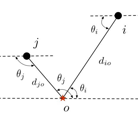
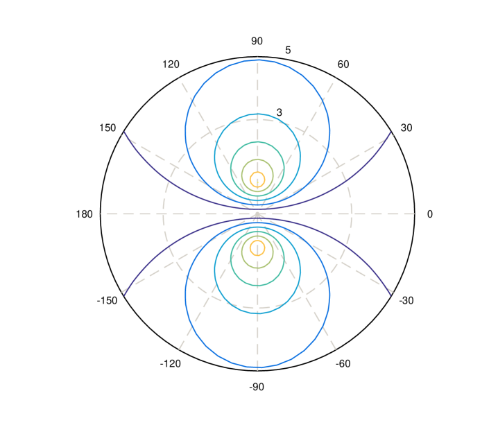
For ease of notation, we represent the relative sensor-target position and sensor-target orientation in polar coordinates with the target at the center:
| (8) |
where , , and indicate the relative distances and orientations between sensors and target as shown in Figure 1.
Theorem 4.
The lower bound of the inverse of condition number of the observability matrix for system is given by,
| (9) |
where .
We plot as a function of and angle with and selected as and , respectively (Figure 2). Note that reaches its maximum when and . That is, both sensors are at the same distance from the target and are perpendicular with respect to the target. On the other hand, when , , or , reaches zero. We summarize the results in the following theorem.
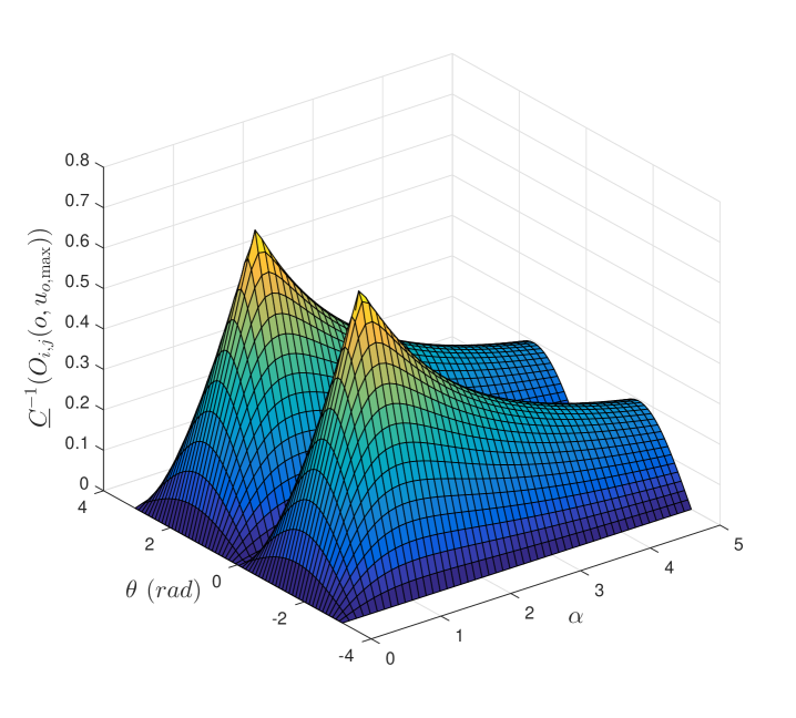
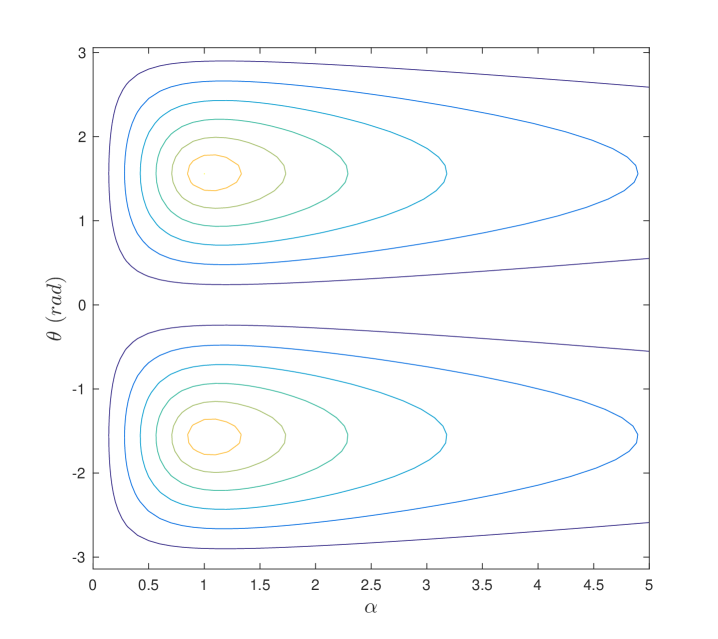
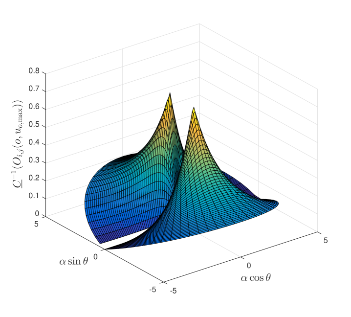
Theorem 5.
The lower bound of the inverse of the condition number for the observability matrix for system, , reaches its maximum, , at and , and reaches its minimum, zero, at , , , or . For a fixed , the minima occurs when or , but the maximum extreme point is not at .
Next, we solve two assignment problems for selecting sensor(s) to track target(s).
IV Assignment Algorithms
So far, we have assumed that we know the true position, , of the target at time . In practice, we only have an estimate, , for along with its covariance . The estimate is obtained by fusing the past measurements obtained by the sensors using, for example, an Extended Kalman Filter (EKF).
Since the sensors know the probability distribution of target’s state with mean , and covariance , they can calculate the relative distances, , by using the Mahalanobis distance [11],
IV-A A –approximation algorithm for Problem 1
We propose a greedy algorithm to solve Problem 1. In each round, we calculate the observability metric, for all triples , and select the triple which has the maximum , then remove from sensor set and remove from target set , respectively. We present the greedy approach in Algorithm 1 where denotes total value charged by the greedy approach. We can use the inverse of the condition number (Equation 9) as .
We present the following lemmas to guarantee the effectiveness of the greedy algorithm.
Theorem 6.
where OPT is the optimal algorithm for Problem 1.
Proof.
Suppose GREEDY picks triple in the round. We will charge the value to at most three triples in OPT that have not been charged in previous rounds. Furthermore, if a triple in OPT is charged in the round, then we show that the value of the triple is less than .
There are three cases.
-
1.
is also chosen by OPT. In this case, we will charge exactly to the triple in OPT, if it has not been charged previously.
-
2.
Exactly two of appear in a triple chosen by OPT. Consider the case where OPT chooses where . All other cases are symmetric. In this case, we need to charge to at most two triples — and the one containing , say . If has not been charged previously, then it must mean that GREEDY has not assigned any sensors to in previous rounds. Since GREEDY chose in the round, it must mean , otherwise GREEDY would have chosen in the round. Likewise, if has not been charged previously, we must have . Therefore, the value charged in the round will be at most twice of .
-
3.
No two of appear in the same triple chosen by OPT. In this case, we can charge the value of to at most three triples. Using an argument similar to the previous case, we can say that the value charged in the round will be at most thrice of .
Therefore, once all triples in GREEDY are charged, it follows that .
IV-B General assignment using Submodular Welfare Optimization
The sensor assignment problem where only two sensors are assigned is discussed above. We now study a more general assignment (Problem 2) where each target is tracked by a subset of sensors whose cardinality is not necessarily two. This is known as submodular welfare problem in the literature[12] where the objective is to maximize for independent sets by using monotone and submodular utility functions . A greedy algorithm [9] yields a –approximation for this problem. We first show that the lower bound of the inverse of the condition number is neither monotone nor submodular which makes the optimization problem much more challenging.
Theorem 7.
The lower bound of the inverse of condition number function is neither monotone increasing nor submodular.
Proof.
We prove the claim by giving two counter-examples.
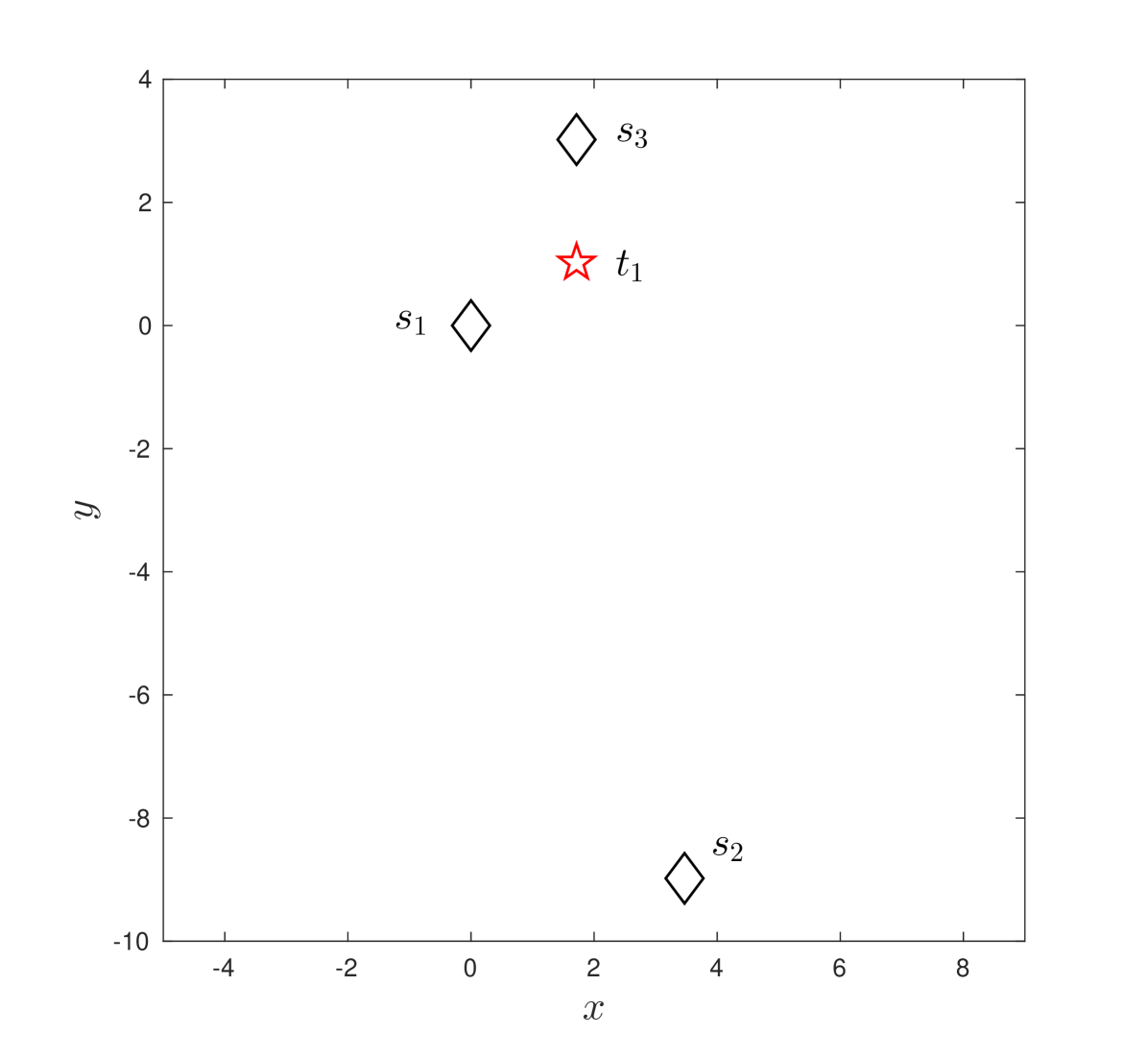
Case 1: Given the sensors , , and target with in 2-D plane (Figure 3-(a)), , which shows is not monotone increasing.
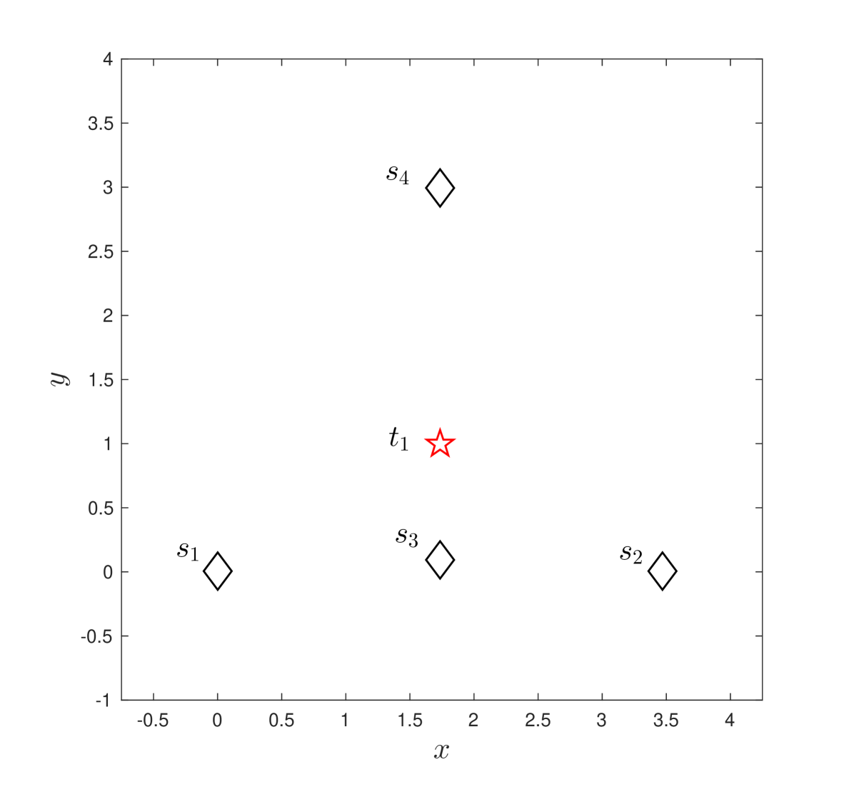
Case 2: Given the sensors , , , and target with in 2-D plane (Figure 3-(b)), , which shows is not submodular.
Therefore, we focus on other measures of observability and summarize the results in Theorem 8.
Theorem 8.
For symmetric observability matrix, , its trace, log determinant, rank and the trace of its inverse are submodular and monotone increasing.
The proof is similar to proving that the trace of the Gramian and inverse Gramian, the log determinant, and the rank of the Gramian are monotone submodular[13]. Resorting to submodular and monotone observability measure, we can use a simpler greedy algorithm to solve the General Assignment Problem.
V Simulations
We illustrate the performance of the pairing and assignment strategies for sensor selection using observability measure as the performance criterion. We first consider the two sensors case for tracking a moving target, and then focus on the multi-sensor multi-target assignment problems. The video444https://youtu.be/Kt0yeYXyrKQ and the code555https://github.com/lovetuliper/observability-based-sensor-assignment.git of our simulations are available online.
V-A Two Sensors Case
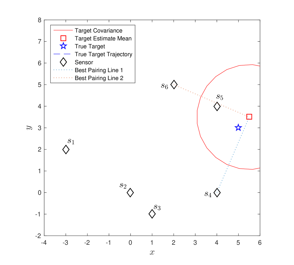
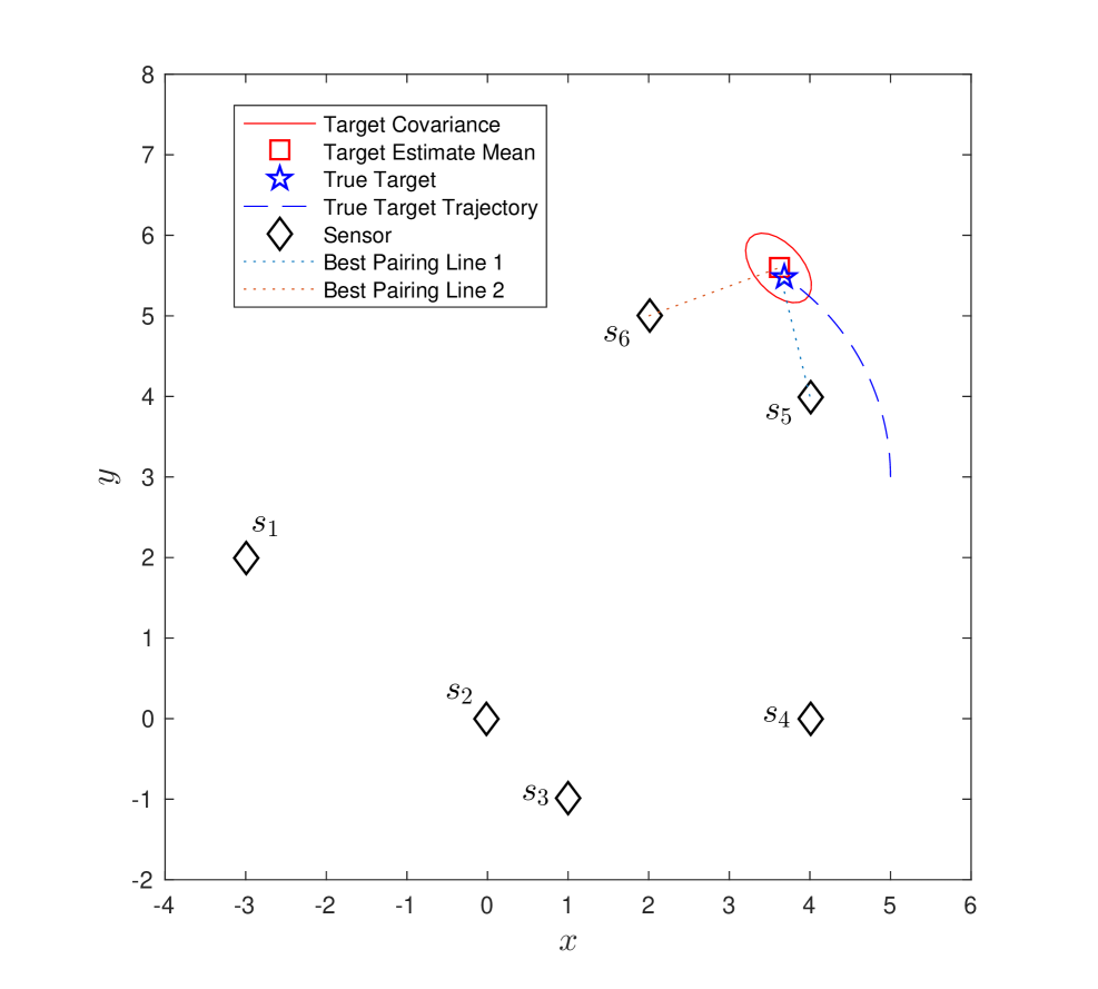
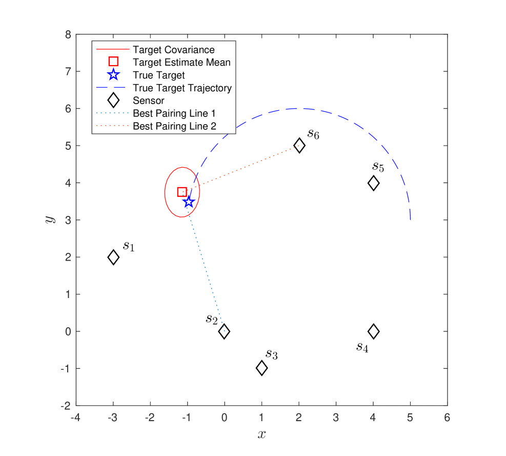
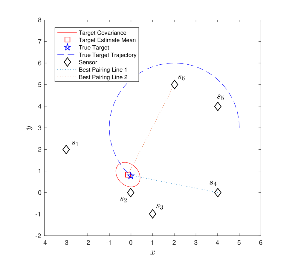
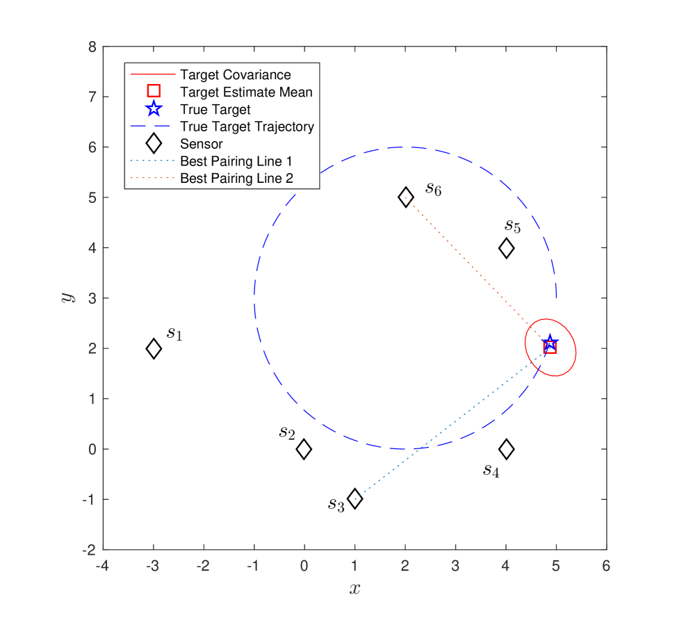
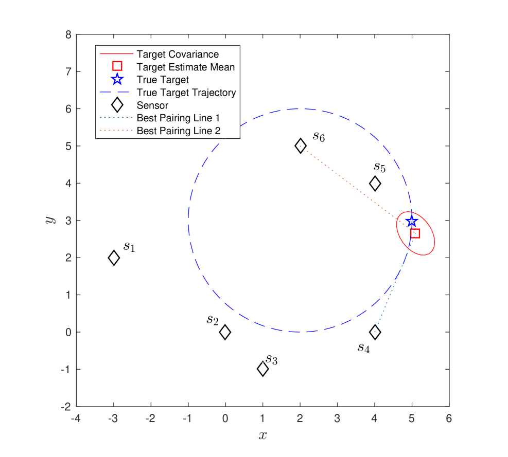
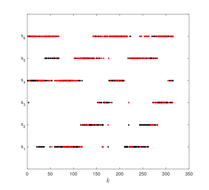
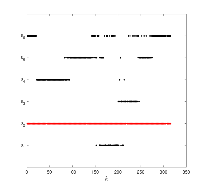
We first consider the scenario where the target is moving independently of six stationary sensors (–). The target follows a circular trajectory with . We compare three strategies: (1) flexible best pair: we pair sensors which have the maximum for tracking the moving target (Figure 5–(a)); (2) flexible pair for fixed sensor: we pair an arbitrarily chosen sensor, , with the best sensor at each timestep (Figure 5–(b)); (3) best-fixed pair: we pair with at all timesteps. We chose since it gives the best performance amongst all other sensors, on an average, for the circular trajectory.
Figure 4–(a) to (f) shows the result of running strategy (1) over timesteps. The best selected pair at each timestep is shown in Figure 5-(a).
We show the results for the three strategies in Figure 6. We plot the inverse of the condition number, the estimation error , and the trace of covariance matrix over time. We observe that the first strategy maintains a higher and has lower and trace of covariance almost all times. Around , the best pair changes frequently as seen in Figure 5-(a).
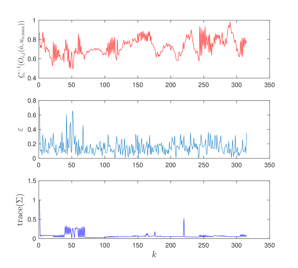
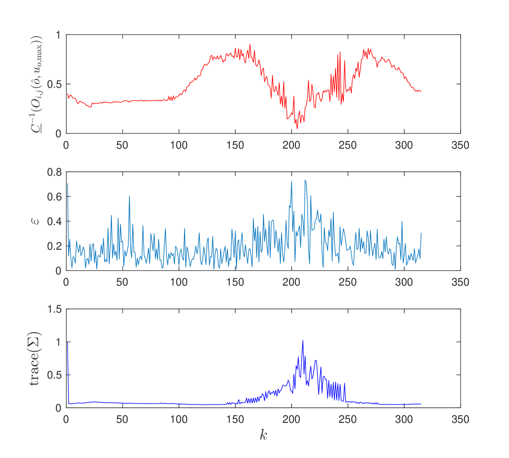
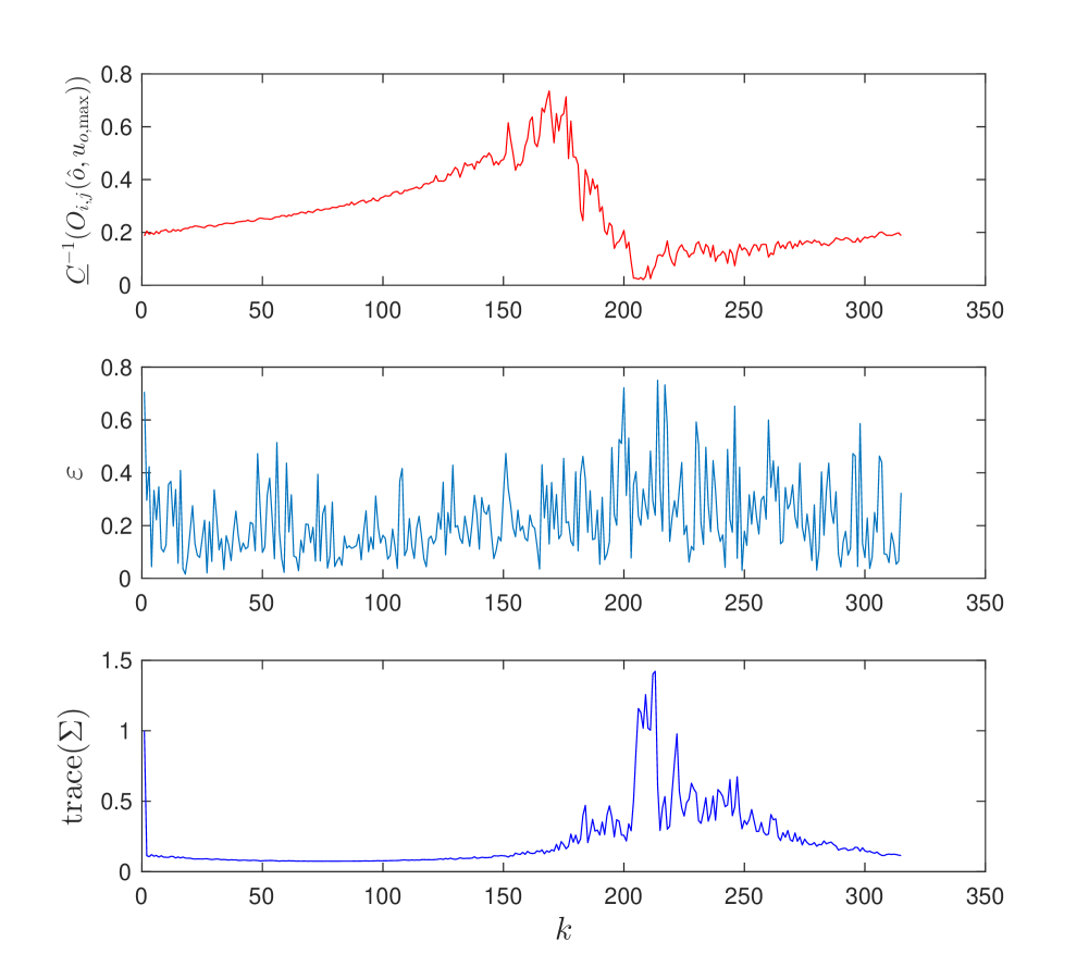
Note that in all three cases, higher correlates with lower and suggesting that the tracking performance can be improved by improving the lower bound of the inverse of the condition number.
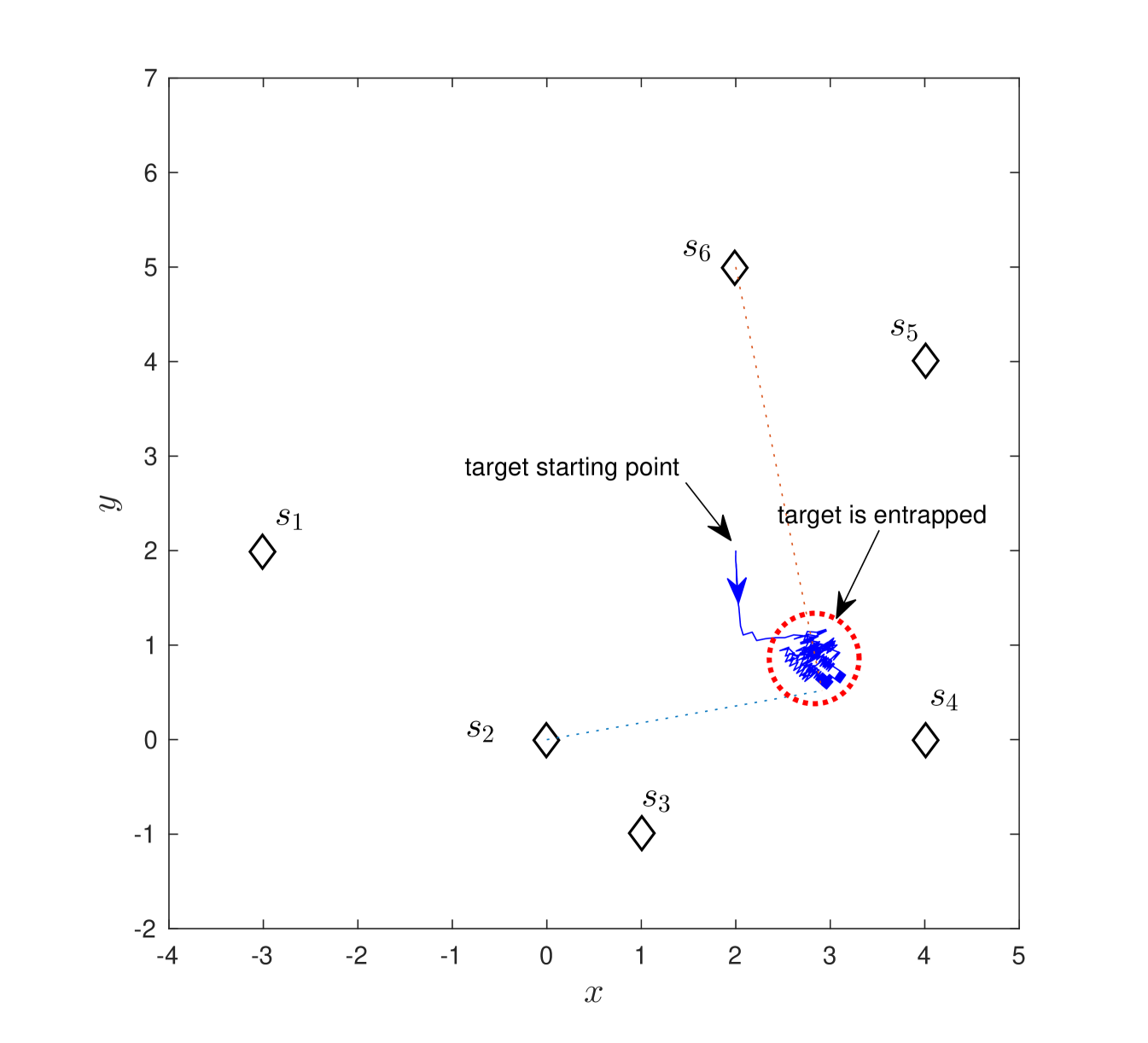
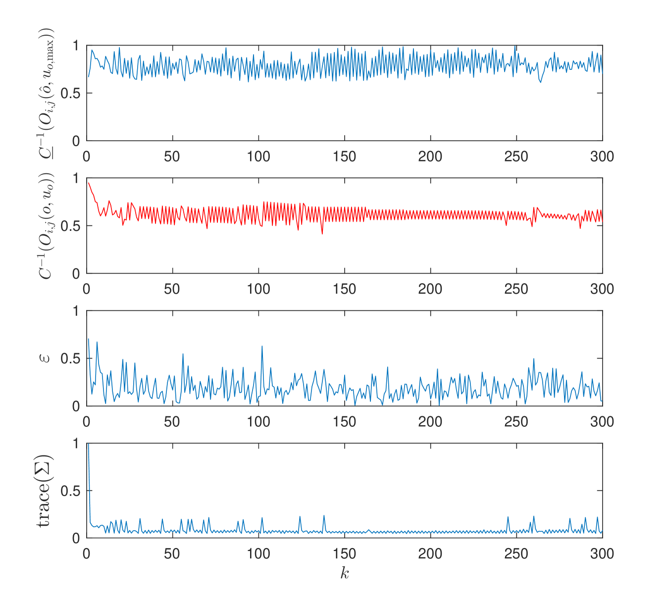
V-B Adversarial Target
We also simulate the scenario where the target moves in an adversarial fashion. At each time step, the target moves in a direction so as to minimize the inverse of the condition number. Here, the target has an advantage in that it knows its own exact state and control input, while sensors only have an estimate. At each timestep, the target evaluates all the possible control inputs within a ball of radius , around itself and chooses on that minimizes .
Figure 7 shows an instance where the target is “trapped” by the sensors. The target fails to reduce the inverse of the condition number since the sensor pair switches whenever the target gets closer to a sensor.
V-C Greedy Unique Pair Assignment
The Unique Pair Assignment problem is NP-Complete. Therefore, finding is infeasible in polynomial time. In order to empirically evaluate the Greedy Unique Pair Assignment (Algorithm 1), we resort to a new assignment scenario where each sensor can be matched in multiple different pairs and each sensor pair can be assigned to at most one specific target. We formulate the new assignment as Relaxed Pair Assignment (Problem 3). It is clear that solving Relaxed Pair Assignment problem optimally gives us an upper bound of optimality for Unique Pair Assignment problem. We can use this upper bound for the comparison of the greedy approach in Unique Pair Assignment.
Problem 3 (Relaxed Pair Assignment).
Given a set of sensor positions, and a set of target estimates at time , , find an assignment of unique pairs of sensors to targets:
| (10) |
with the added constraint that all pairs are unique, that is, , , and/or .
The Relaxed Pair Assignment problem can be solved optimally by using maximum weight perfect bipartite matching (MWPBM) [14]. Note that a sensor can be matched in multiple distinct pairs and assigned to multiple targets. The MWPBM can be solved using the Hungarian algorithm [15] in polynomial time.
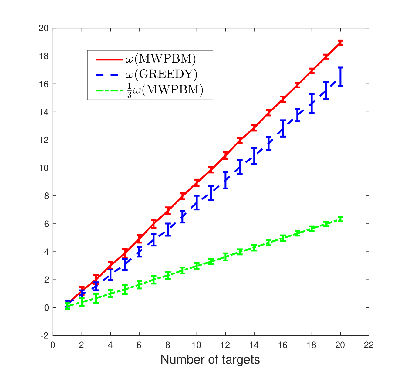
In order to see the effectiveness of the greedy algorithm in Unique Pair Assignment, we compare the total value charged by the greedy algorithm, , with the total value charged by the MWPBM, , in Relaxed Pair Assignment as shown in Figure 8. We consider different number of targets with for 1 to 20 and set the number of robots, . For each , the positions of sensors and targets are randomly generated within for 30 trials. Set the maximum control input for each target as . Figure 8 shows that is close to and much higher than . Thus, even though we give a theoretical –approximation for the greedy algorithm, it performs much better in practice.
V-D General Pair Assignment
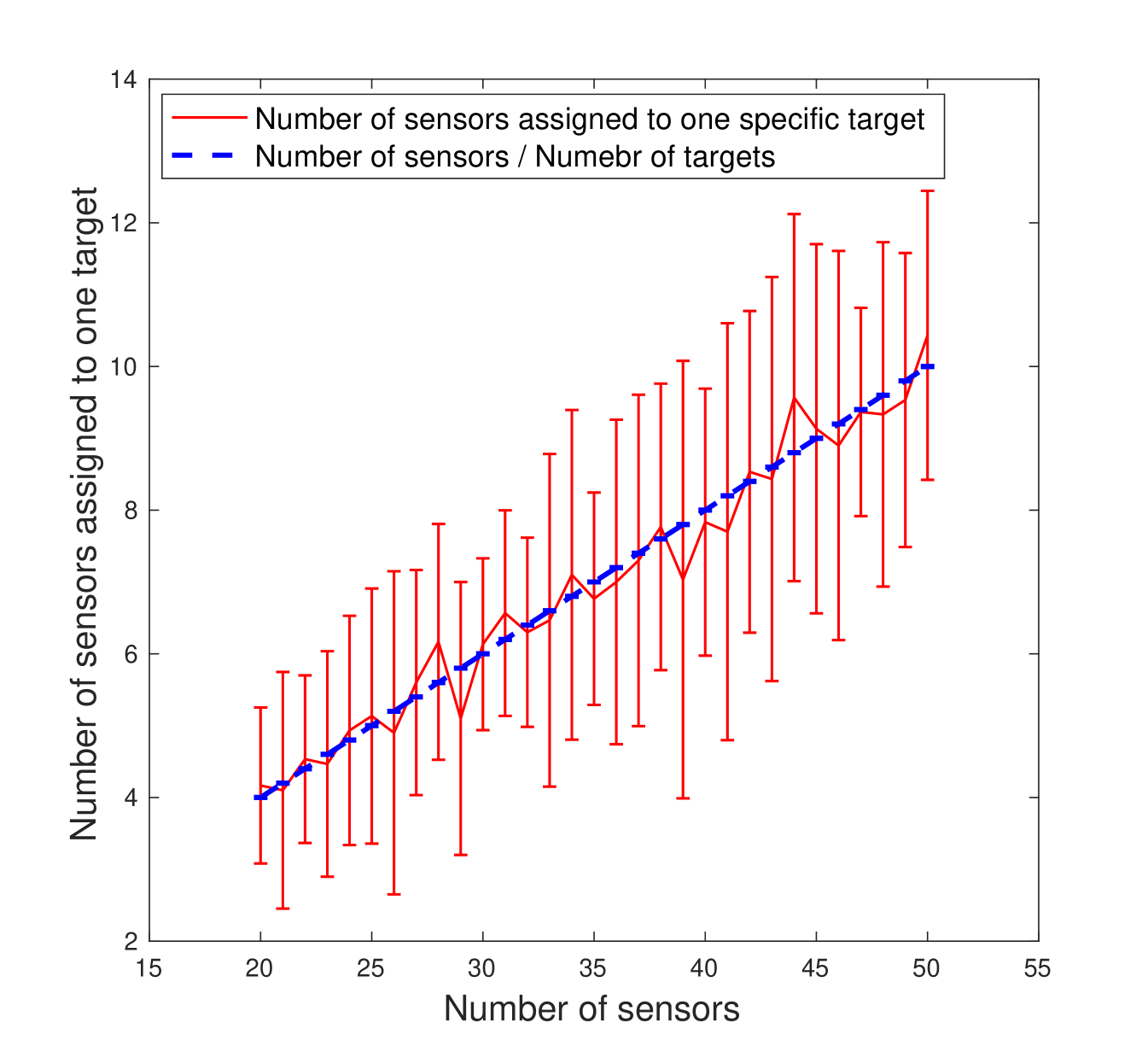
We also simulate the greedy assignment [9] for the General Assignment problem by using log determinant of symmetric observability matrix, as observability measure. We set the number of targets as and number of sensors from 20 to 50. For each , the positions of sensors and targets are randomly generated within for 30 trials. We compare the number of sensors assigned to one specific target, i.e., with the as shown in Figure 9. It shows that the sensors are assigned to each target almost evenly.
VI Conclusion
In this paper, we solved sensor assignment problems to improve the observability for target tracking. We derived the lower bound on the inverse of the condition number of the observability matrix for a system with a mobile target and stationary sensors. The lower bound considers only the known part of the observability matrix — the sensor-target relative position and an upper bound on the target’s speed. We showed how this lower bound can be employed for sensor selection. We considered two sensor assignment problems for which we presented constant-factor approximation algorithm. Our immediate work is focused on assigning sensors to cover an area instead of tracking a group of targets. Another avenue is designing an efficient set covering strategy based on observability measures which are submodular and monotone.
References
- [1] M. Montemerlo, S. Thrun, D. Koller, B. Wegbreit, et al., “Fastslam: A factored solution to the simultaneous localization and mapping problem,” in Aaai/iaai, 2002, pp. 593–598.
- [2] H. Durrant-Whyte and T. Bailey, “Simultaneous localization and mapping: part i,” IEEE robotics & automation magazine, vol. 13, no. 2, pp. 99–110, 2006.
- [3] A. S. Gadre and D. J. Stilwell, “Toward underwater navigation based on range measurements from a single location,” in Robotics and Automation, 2004. Proceedings. ICRA’04. 2004 IEEE International Conference on, vol. 5. IEEE, 2004, pp. 4472–4477.
- [4] G. Papadopoulos, M. F. Fallon, J. J. Leonard, and N. M. Patrikalakis, “Cooperative localization of marine vehicles using nonlinear state estimation,” in Intelligent Robots and Systems (IROS), 2010 IEEE/RSJ International Conference on. IEEE, 2010, pp. 4874–4879.
- [5] F. Arrichiello, G. Antonelli, A. P. Aguiar, and A. Pascoal, “An observability metric for underwater vehicle localization using range measurements,” Sensors, vol. 13, no. 12, pp. 16 191–16 215, 2013.
- [6] R. K. Williams and G. S. Sukhatme, “Observability in topology-constrained multi-robot target tracking,” in Robotics and Automation (ICRA), 2015 IEEE International Conference on. IEEE, 2015, pp. 1795–1801.
- [7] R. Hermann and A. Krener, “Nonlinear controllability and observability,” IEEE Transactions on automatic control, vol. 22, no. 5, pp. 728–740, 1977.
- [8] A. J. Krener and K. Ide, “Measures of unobservability,” in Decision and Control, 2009 held jointly with the 2009 28th Chinese Control Conference. CDC/CCC 2009. Proceedings of the 48th IEEE Conference on. IEEE, 2009, pp. 6401–6406.
- [9] G. L. Nemhauser, L. A. Wolsey, and M. L. Fisher, “An analysis of approximations for maximizing submodular set functions—i,” Mathematical Programming, vol. 14, no. 1, pp. 265–294, 1978.
- [10] P. Tokekar, J. Vander Hook, and V. Isler, “Active target localization for bearing based robotic telemetry,” in Proceedings of IEEE/RSJ International Conference on Intelligent Robots and Systems. IEEE, 2011, pp. 488–493.
- [11] P. C. Mahalanobis, “On the generalized distance in statistics,” Proceedings of the National Institute of Sciences (Calcutta), vol. 2, pp. 49–55, 1936.
- [12] J. Vondrák, “Optimal approximation for the submodular welfare problem in the value oracle model,” in Proceedings of the fortieth annual ACM symposium on Theory of computing. ACM, 2008, pp. 67–74.
- [13] T. H. Summers, F. L. Cortesi, and J. Lygeros, “On submodularity and controllability in complex dynamical networks,” IEEE Transactions on Control of Network Systems, vol. 3, no. 1, pp. 91–101, 2016.
- [14] T. H. Cormen, Introduction to algorithms. MIT press, 2009.
- [15] H. W. Kuhn, “The hungarian method for the assignment problem,” Naval research logistics quarterly, vol. 2, no. 1-2, pp. 83–97, 1955.
- [16] G. Strang, Linear algebra and its applications. Academic Press, 1976.
- [17] J. N. Franklin, Matrix theory. Courier Corporation, 2012.
Proof for Theorem 1
Proof.
We partition into the known and unknown parts as,
| (11) |
where
| (12) |
and
| (13) |
indicate the contribution to the observability matrix from sensor-target relative state and target’s control input, respectively.
The singular values of can be found as the square-root of the eigenvalues of the symmetric observability matrix, , given as [16],
| (14) | |||||
| (15) |
We can use Weyl and dual Weyl inequalities to bound the singular values. For Hermitian matrices and with eigenvalues written in increasing order and , respectively, the Weyl inequalities[17] is given by,
| (16) |
where and . Similarly, the dual Weyl inequalities is given by
| (17) |
where and .
Since , and are symmetric matrices, they are Hermitian with the eigenvalues (in ascending order) as , and . Following the Weyl and dual Weyl inequalities, we get
| (20) | |||
| (23) |
Thus,
| (24) |
Then, from Equation 15 and Equation 24, the inverse of the condition number of the local nonlinear observability matrix,
By calculating the eigenvalues of symmetric matrix of target’s control contribution,
we get,
| (25) |
Then the lower bound of is calculated as
| (26) | |||||
Equation 26 gives the main lower bound. Note that cannot be determined since target’s control input, , is unknown. However, we know that . Therefore,
| (27) |
This yields our main lower bound result.
Proof for Theorem 2
Proof.
The local observability matrix for one-sensor-target, system can be derived from Equation 5 as,
| (28) |
The sensor-target relative state contribution is.
The system is weakly locally observable if has full column rank, i.e., . However, the sensor does not know the target’s control input, .
From the eigenvalues of symmetric matrix of sensor-target relative state contribution of system given by,
we get,
| (29) |
Thus, from Equation 26, the lower bound for is . Consequently, the lower bound cannot be controlled by the sensor.
Proof for Theorem 3
Proof.
Recall that . We have,
| (30) |
Following Equations 24 and 25, we have the lower bound for , described as
| (31) |
The observability can be improved by increasing this lower bound. We can transform the statement of the theorem (using eigenvalues instead of singular values) as: if
| (32) |
then
| (33) |
where the and denotes the eigenvalues before and after the sensors’ apply their control, respectively.
Remark 2.
Equation 32 is sufficient, but not necessary condition to guarantee Equation 33. This is because Equation 33 can be established with a weaker condition,
We choose the stricter condition (Equation 32) because it is conceptually easy to separate and eliminate the influence on the degree of observability from target’s control input, , which is unknown and uncontrolled.
Proof for Theorem 4
Proof.
The sensor-target relative state contribution of the local observability matrix (Equation 7) is,
| (36) |
The lower bound of the inverse of the condition number of is . Our goal is to determine how to improve by analyzing the sensor-target relative state contribution. This is similar to the work presented in [5].
Proof for Theorem 5
Proof.
First, for a fixed ,
and
Thus, when is fixed, reaches its minimum, , and reaches its maximum . Then, when ,
and
Therefore, reaches its minimum , at , or , and reaches its maximum , at , as shown in Figure 2 where, reaches its maximum at and .
Note that, when , is always null and not influenced by . Besides, for a fixed , the minimum extreme point w.r.t. still happens when or , but the maximum extreme point is not at , which is shown is the following derivations.
and
| (39) |
Since
also reaches its minimum at or . However, cannot make Equation 39 established when , and thus, the extreme point is not at .