A machine learning photon detection algorithm for coherent X-ray ultrafast fluctuation analysis
Abstract
X-ray free electron laser (XFEL) experiments have brought unique capabilities and opened new directions in research, such as creating new states of matter or directly measuring atomic motion. One such area is the ability to use finely spaced sets of coherent x-ray pulses to be compared after scattering from a dynamic system at different times. This enables the study of fluctuations in many-body quantum systems at the level of the ultrafast pulse durations, but this method has been limited to a select number of examples and required complex and advanced analytical tools. By applying a new methodology to this problem, we have made qualitative advances in three separate areas that will likely also find application to new fields. As compared to the ‘droplet-type’ models which typically are used to estimate the photon distributions on pixelated detectors to obtain the coherent X-ray speckle patterns, our algorithm pipeline achieves an order of magnitude speedup on CPU hardware and two orders of magnitude improvement on GPU hardware. We also find that it retains accuracy in low-contrast conditions, which is the typical regime for many experiments in structural dynamics. Finally, it can predict photon distributions in high average-intensity applications, a regime which up until now, has not been accessible. Our AI-assisted algorithm will enable a wider adoption of x-ray coherence spectroscopies, by both automating previously challenging analyses and enabling new experiments that were not otherwise feasible without the developments described in this work.
I Introduction
The construction and operation of X-ray free electron lasers (XFELs) Decking et al. (2020); Prat et al. (2020); Kang et al. (2017); Ishikawa et al. (2012); Emma et al. (2010) has enabled a great leap towards deeper understanding of a diverse area of scientific research areas Bostedt et al. (2016), including planetary science Vinko et al. (2012), astrophysics Bernitt et al. (2012), medicine Redecke et al. (2013) and molecular chemistry Wernet et al. (2015). With the unprecedented brightness, short pulse duration, and x-ray wavelengths, new states of matter can be created and studied Lee et al. (2021), while dynamics can be monitored, and now controlled, on ultrafast timescales Wandel et al. (2022).
With the start of high repetition rate next-generation light sources, methods which have so far been challenging will become feasible, such as resonant inelastic x-ray scattering at high time- and spectra- resolution Ament et al. (2011) and x-ray photoemission spectroscopy Siefermann et al. (2014). One such example is X-ray photon correlation spectroscopy (XPCS) Sutton (2008); Shpyrko et al. (2007), which uses the spatial coherence of the X-ray beam to produce a scattering ‘fingerprint’ of the sample. This fingerprint, or speckle pattern, can be correlated in time to directly observe equilibrium dynamics of a given system. This information of the thermal fluctuations can be related back the energetics and the interactions in the system. This is typically measured by calculating the intensity-intensity autocorrelation function and extracting the intermediate scattering function (Equation 1),
| (1) |
which allows the time correlation to be related back to the physical properties of the system being studied.
Another benefit of these new machines is in their ability to produce finely spaced X-ray pulses with controllable delay, using X-ray optics Sun et al. (2019) or special modes of the accelerator Decker et al. (2022). These pulses enable studies of spontaneous fluctuations at orders of magnitude faster timescales than what is possible using XPCS at x-ray synchrotron facilities, with one key area of application being emergent phenomena in quantum materials. We refer to this multi-pulse adding technique here as X-ray photon fluctuation spectroscopy (XPFS) Shen et al. (2021). This is a unique tool which differs from traditional pump-probe spectroscopy which detects the relaxation from a non-equilibrium state, by instituting more of a ‘probe-probe’ method, where fluctuations in the equilibrium state can be measured directly by comparing how the system changes between probe pulses. Here, one adds the pulses which are too close together in time to be read out by the detector Gutt et al. (2009) and uses statistics of the coherent speckle Goodman (2007) to compute the fluctuation spectra using the contrast Decaro et al. (2014); Bandyopadhyay et al. (2005), i.e. the fast dynamical information of the system can be distinguished by studying single photon fluctuations. Even with the massive amount of photons per pulse, three things typically result in a single photon detection process: the decrease of intensity after the scattering process on a single pulse basis, the short pulse duration, and the sometimes reduced intensity required to ensure excitations are not produced in the sample.
In principle, if the discrete distribution of photon counts over the detector can be accurately measured and enough samples averaged, it is possible to determine the dynamical evolution the sample by computing the speckle contrast as a function of delay-time and momentum transfer . The contrast is obtained by fitting a negative binomial distribution parameterized by = and the average number of photons per pixel Hruszkewycz et al. (2012) – i.e. :
| (2) |
Fitting this negative binomial distribution requires the extraction of photon counts from raw detector images, and works fairly well in the hard x-ray regime and for large pixel size detectors Hruszkewycz et al. (2012); Sikorski et al. (2016); Sun et al. (2020). In cases where the pixels are small, or the energy of the x-rays is much lower, this process can involve additional obstacles. One challenge is the point spread function of a single photon can spread non-uniformly over many pixels. This is especially true in the soft x-ray regime, where there can be a large variability in the charge cloud size – owing to variable diffusion lengths within a pixel – and low signal to noise ratios. These effects have recently been shown to be corrected by a variational droplet model called the Gaussian Greed Guess (GGG) droplet model Burdet et al. (2021a), which can fit the large variation in charge cloud radii to produce discrete images where each pixel contains the number of corresponding photons.
While ’droplet-type’ models have been largely successful, there is a need to increase the speed of these computational models as well as to handle common scenarios, such as low signal-to-noise. A few works have employed machine learning techniques to address some of these outstanding challenges. For instance, the use of convolutional neural networks to analyze XPCS data for well-resolved speckles has showed the denoising approaches are able to achieve significantly better signal-to-noise statistics as well as estimations of key parameters of interest Campbell et al. (2021); Konstantinova et al. (2022, 2021). Previous work has also considered the single-photon analysis for hard X-ray detectors using machine learning. One approach Blaj, Chang, and Kenney (2019) has been to use a tensorflow computational graph with hand-crafted convolutional masks derived from an in-depth study of photon physics at semiconductor junctions Blaj et al. (2017). This implementation is extremely fast, but does not apply to regimes where there may be a large number of photons per droplet. Another method Abarbanel (2019) proposes a feed-forward neural network architecture, based on a sliding prediction of 5x5 regions of the input image. This was proposed for the photon map prediction task and is shown to be applicable for hard X-ray, low count rate experiments. However, additional factors such as noise, low photon energies, and insufficient signal-to-noise ratios can cause limitations in this methodology and thus obscure scientific results. Furthermore, in cases where a higher intensity can be measured, the charge clouds can quickly coalesce, making this problem intractable.
In this work, we expand the applicability of this ultrafast method by demonstrating robust single-shot prediction using an AI-assisted algorithm in the soft X-ray regime for data with relatively high average count-rates and significant charge sharing. This is carried out using a fully convolutional neural network architecture Long, Shelhamer, and Darrell (2015), which we compare against the GGG method, currently the best algorithm for soft X-ray analysis using small pixel-size detectors Burdet et al. (2021a). We find that we are able to access a new phase space of measurement parameters that, until now, has not been accessible in structural dynamics studies using this method. Our algorithm enables a two order of magnitude speedup on appropriate hardware, is relative accurate for low contrast cases, and is stable at higher intensities than the GGG algorithm. We first describe the machine learning model and simulator used to train it, specifying the architecture, how the model is trained, and the evaluation metric used. This is followed by our main results, and the three areas which were shown to return excellent results relative to the current state-of-the-art models. Finally, we end with a discussion of uncertainty quantification, and how one can judge the error for different models.
II Modelling and Analysis Approach
II.1 Simulator Description
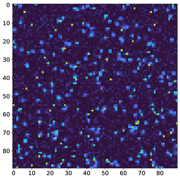
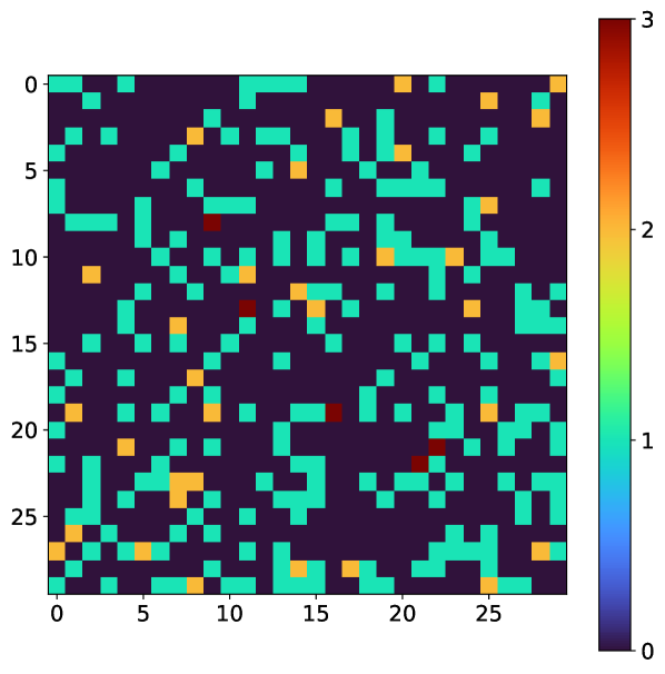
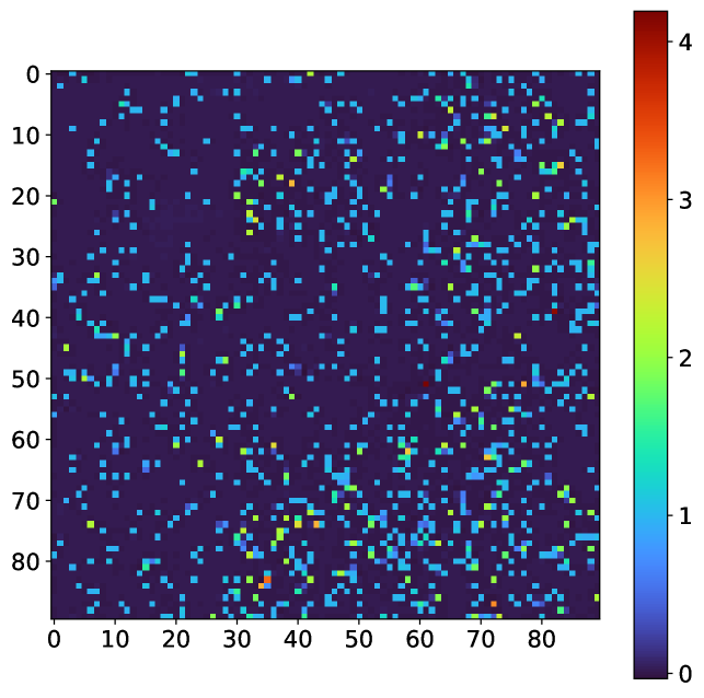
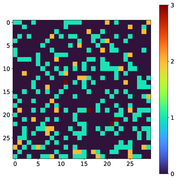
One key issue in the development of supervised machine learning algorithms is a robust simulator which can adequately describe the data. To describe the simulator here, we denote an input XPFS frame as and the corresponding output photon map as . The 3x3 reduction in dimensionality between and is used to mimic the speckle oversampling factor that is typically used in LCLS experiments. The final calculations are performed on a 30x30 image to allow for the proper photon events to be expressed per speckle.
The detector images and corresponding photon maps are simulated according to the exact parameters described in Burdet et al. (2021a) which were tuned to mimic a previous experiment by matching the overall pixel and droplet histogram. To simulate ground truth photon maps, the following ranges were used: [0.025, 2.0] and [0.1, 1.0]. The relevant detector parameters are the probabilities () and sizes () of the photon charge clouds, the variance of the zero-mean Gaussian background detector noise () and the total number of analog-to-digital units (ADUs) per photon. These parameter values are reproduced below in Table 1 and an example of a detector image / photon map pair is shown in Figure 1. For comparison, we used the Gaussian Greedy Guess (GGG) algorithm with relevant parameters which were optimized for these specific simulation parameters described above Burdet et al. (2021a).
| Number of pixels per droplet | 1 | 2 | 3 | 4 | 5 | 6 | 7 | 8 |
| 0.10 | 0.25 | 0.35 | 0.45 | 0.55 | 0.60 | 0.65 | 0.70 | |
| 0.20 | 0.125 | 0.125 | 0.175 | 0.175 | 0.10 | 0.05 | 0.025 | |
| photon ADU = 340 | = [0-12] ADU | |||||||
II.2 Model Architecture
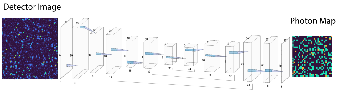
In this problem, we seek a supervised machine learning model which learns the functional mapping , from paired simulated data points (). In this case, the functional mapping was chosen to be a U-Net neural network (Figure 2), a fully convolutional autoencoder architecture, which is characterized by having skip-connections between different layers of resolution and has been shown to perform well on various image segmentation tasksRonneberger, Fischer, and Brox (2015). In the schematic in Figure 2, the architecture is outlined via successive "convolutional blocks". Each such convolutional block consists of two convolutional layers sequentially applied to the input. After each convolution, we utilize batch normalization Ioffe and Szegedy (2015) to ensure robust optimization, followed by a Rectified Linear Unit (ReLU) activation.
II.3 Training Details and Validation Metrics
To train the model, we use the Frobenius norm between the predicted photon maps () and the true photon maps (). This loss function measures the average squared deviation between the predicted photon map and the true photon map, where the average is taken both within a given frame (which contains pixels) and between frames () in the dataset.
| (3) |
The U-Net model is trained by minimizing with respect to the model parameters. To train the neural network, we use the following hyperparameters: Adaptive Moment Estimation (ADAM) algorithm for optimization Kingma and Ba (2014), batch size = 128, learning rate = 0.001, and batch normalization. We used NVIDIA A100 GPU hardware with the Keras API Chollet et al. (2015).
We performed analysis at low and high count rates () and trained respective models. For the low- data, 100,000 training data points were simulated based on the detector parameters in Table 1 and uniformly selecting in range [0.025, 0.2] and over the range [0.1, 1.0]. For the high- analysis, 300,000 data points were used for training with an equal proportion of datapoints coming from [0.025, 0.2], [1.0, 2.0] and [0.025, 2.0], respectively, with the the randomly chosen from the range [0.1, 1.0]. To select between competing trained models, the optimal neural network was selected based on maximizing the correlation between the estimated and the true contrast on held-out validation sets of size 5000 for contrast values in the range [0.1, 1.0] with increments of . Here, it is worth emphasizing that the metric used to evaluate the photonizing task is important. For example, the overall accuracy is not necessarily a good metric since many photon maps have a small number of photons. Therefore, a model which uniformly predicts for each pixel will show a uninformatively high accuracy, which is clearly not the desired performance and will lead to poor statistics. Similar issues have been documented in problems with high class imbalances Luque et al. (2019), and correlation based similarity metrics for evaluation are recommended therein Herlocker et al. (2004). Since our final goal is to obtain a good estimate of the contrast, it is useful to use this information directly in the evaluation metric. For the low- analysis, validation datasets were simulated in the range [0.025-0.2]. For the high- analysis, two additional datasets corresponding to in the ranges [1.0, 2.0] and [0.025, 2.0] were used. The evaluation metric for this analysis was the average correlation for the three different ranges. An example of a sample validation plot is shown in Appendix A.
Finally, to obtain an estimate of the contrast from the predicted photon maps we use the maximum likelihood estimation procedure on the negative binomial distribution. In general, the negative binomial distribution is a function of both and . However, we directly use a per-image estimate for and therefore the MLE procedure reduces to a 1D optimization in Roseker et al. (2018).
III Results and Analysis
III.1 Speed of Inference
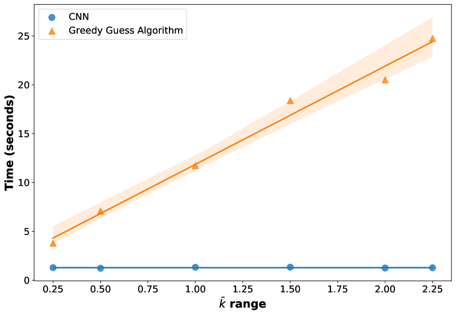
As X-ray sources and detectors move towards faster repetition rates nearing 1 MHz, it is important to preserve the possibility of live data analysis. Here, we compare the speed of an optimized GGG droplet algorithm Burdet et al. (2021b) against the trained CNN model (see Table 2). On 1 CPU, the CNN outperforms the GGG algorithm by roughly an order of magnitude. This advantage stretches to two orders of magnitude when comparing GGG parallelized across multiple CPU cores to the CNN running on one NVIDIA A100 GPU.
| Device | Algorithm | Rate (kHz) | Rate relative to 1 CPU |
|---|---|---|---|
| 1 CPU | GGG | 0.008 | 1 |
| 12 CPU | GGG | 0.05 | 6 |
| 32 CPU | GGG | 0.1 | 12 |
| 1 CPU | CNN | 0.2 | 27 |
| 1 GPU | CNN | 5.0 | 700 |
The observed speedup presented here is consistent with intuition. At inference, the trained neural network, which consists primarily of matrix multiplication operations, is efficiently parallelized over thousands of GPU processes Kirk and Wen-Mei (2016). In contrast, the GGG algorithm requires for-loop operations at the level of each droplet. For this reason, one additional beneficial property of the CNN model is that the prediction rate does not depend on the content of the XPFS frames and is consequently independent of . In contrast, for the GGG algorithm, the run time scales linearly with (Figure 3). Here, it is worth mentioning that the GGG algorithm is already orders of magnitudes faster than the Droplet Least Squares algorithm Hruszkewycz et al. (2012), which is exponential in computational complexity.
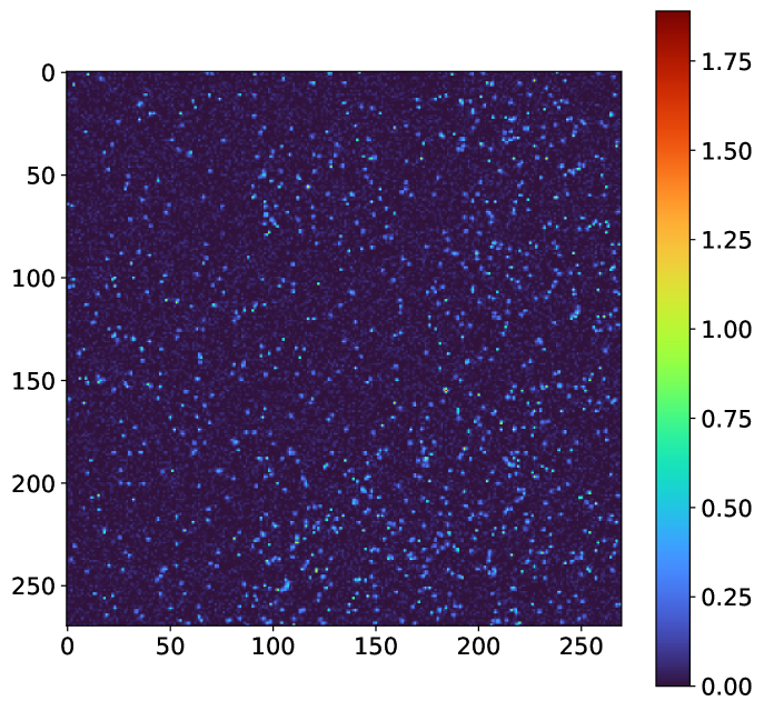
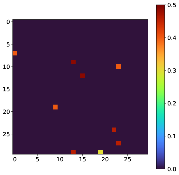
Finally, since the neural network architecture follows a fully convolutional paradigm, it is possible to make predictions on large input / detector sizes than those used in the training set. This is enabled by the fact that fully-convolutional architectures learn local spatial filters which apply to the full image, making the learning process relatively efficient. For this analysis, the neural network can handle input sizes of (, 90, 90, 1), where , are positive integers and denotes a variable number of frames. Note, that this allows for any detector size to be used after zero-padding to nearest (90, 90) frame size. We calculate the average time to make predictions on datasets of dimensionality [100, 90, 90, 1], [100, 270, 270, 1] and [100, 900, 900, 1]. We observe rates of 3.4, 3.1 and 0.3 kHz, respectively. As the rate only decreases a factor of 10 between a frame size of (90,90) and (900,900), it appears that we do not observe quadratic scaling that would be observed using droplet-based algorithms. Furthermore, the ability to analyze such data in a single-shot manner is a significant advantage over the sliding approach for droplet analysis which has been developed Abarbanel (2019). A representative example of the CNN prediction using an input resolution of 270x270 pixels is shown in Figure 4.
III.2 Accuracy
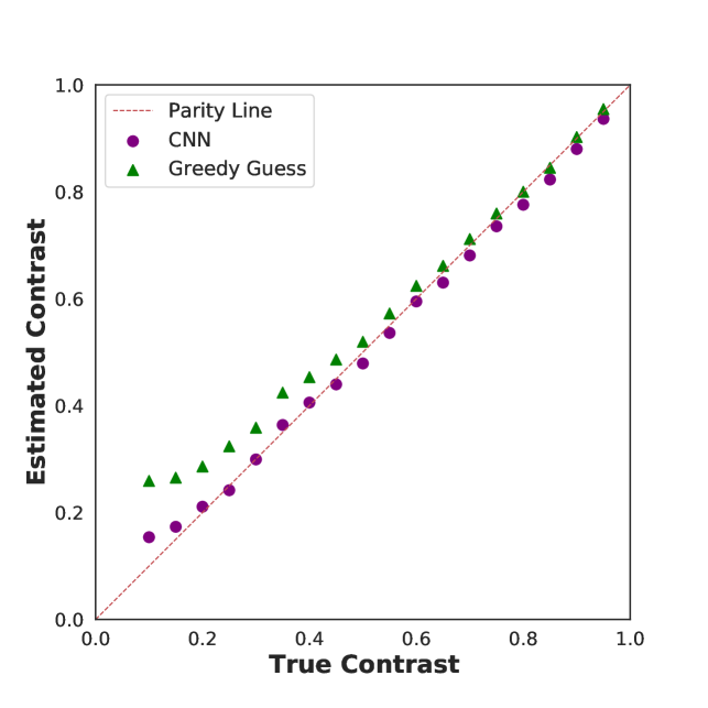
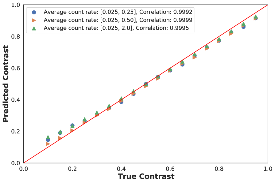
In this section, we compare the prediction quality of the CNN model against the GGG algorithm on data which simulates LCLS experiments and for which the ground truth contrast is known Burdet et al. (2021a). We begin with an analysis of low count-rate ( [0.025, 0.2]) data and subsequently present results for higher count-rate data ( [0.2, 2.0]). To quantify performance, we show parity plots for the predicted and true contrast on datasets with varying contrasts.
At low and high contrasts, the CNN and GGG algorithm give good predictions for the contrast. Although, it is worth pointing out that in this regime the CNN algorithm systematically underpredicts the contrast and has a slightly larger bias than the GGG algorithm. However, at low contrast levels, the GGG algorithm exhibits much greater bias than the CNN (Figure 5a). One possible reason for the overall superior performance of the CNN is that it takes into account variation in photon charge cloud sizes during training. Here, it is worth emphasizing that even after optimizing droplet parameters on simulated data with known detector parameters, the GGG algorithm still exhibits large bias for lower contrast values, indicating that the algorithm may not have the complexity required to fully treat such data.
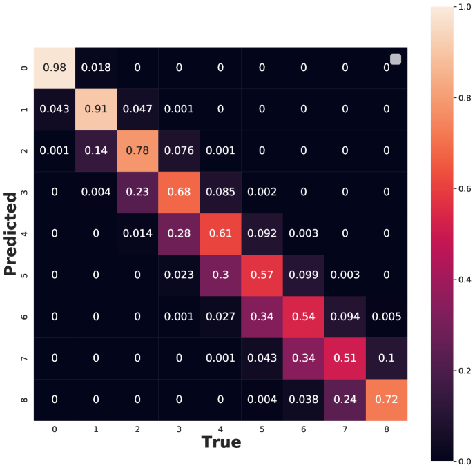
As increases, the CNN performance decreases on an average photon map accuracy basis (Figure 5c). To further examine the CNN errors, we clipped the output photon map to the range of [0,8] (i.e. no photon map has more than eight photons or less than zero photons) and analyzed the confusion matrix (CFi,j) of the predictions (Figure 5d). The diagonal of the confusion matrix represents per-class accuracy. For instance, CF2,2 represents the accuracy of prediction for pixels containing two photons. By examining the diagonal elements, it is clear that the CNN model makes a greater proportion of errors for higher photon counts; note the trend does not hold for the eight photon event due to the clipping operation. The off-diagonals of the confusion matrix indicate how the model makes errors. For example, the CF3,6 term indicates the probability of the model assigning three photons to a pixel when the true number of photons was actually equal to six. From these elements, we see that the CNN tends to systematically under-predict high photon events. Taken together, these observations suggest that there is a dataset imbalance issue owing to the fact that low photon events are more probable in the training set.
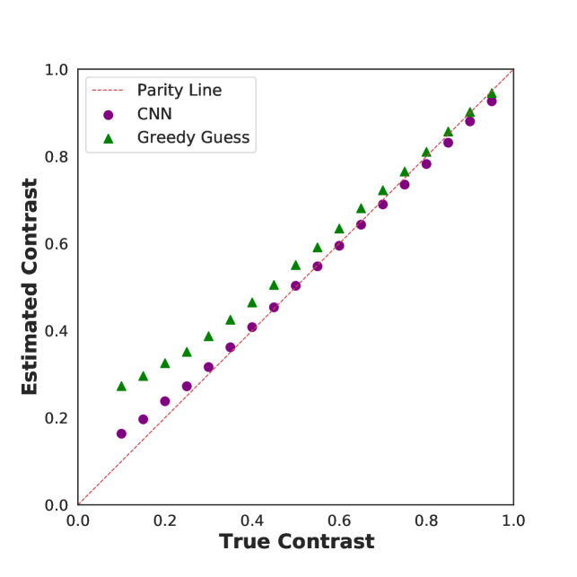
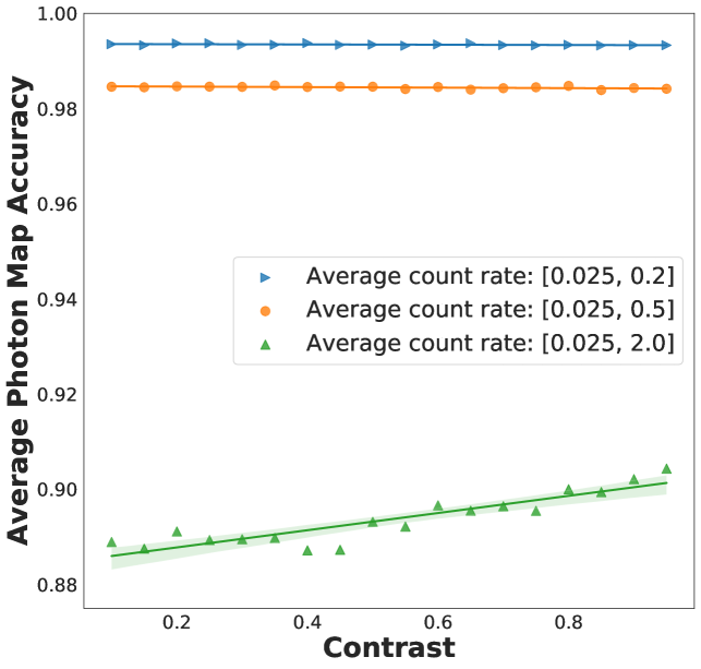
Although at high , the CNN is less accurate on a per-photon map basis (relative to its low performance), this does not necessarily imply inferior contrast predictions. In fact, the parity plots are similar for low and high cases (Figure 5b). This observation stems from the trade-off between information content and accuracy at high (Appendix B). For a fixed dataset size, it is harder to estimate photon counts correctly, but the counts have significantly more information about the unknown parameter.
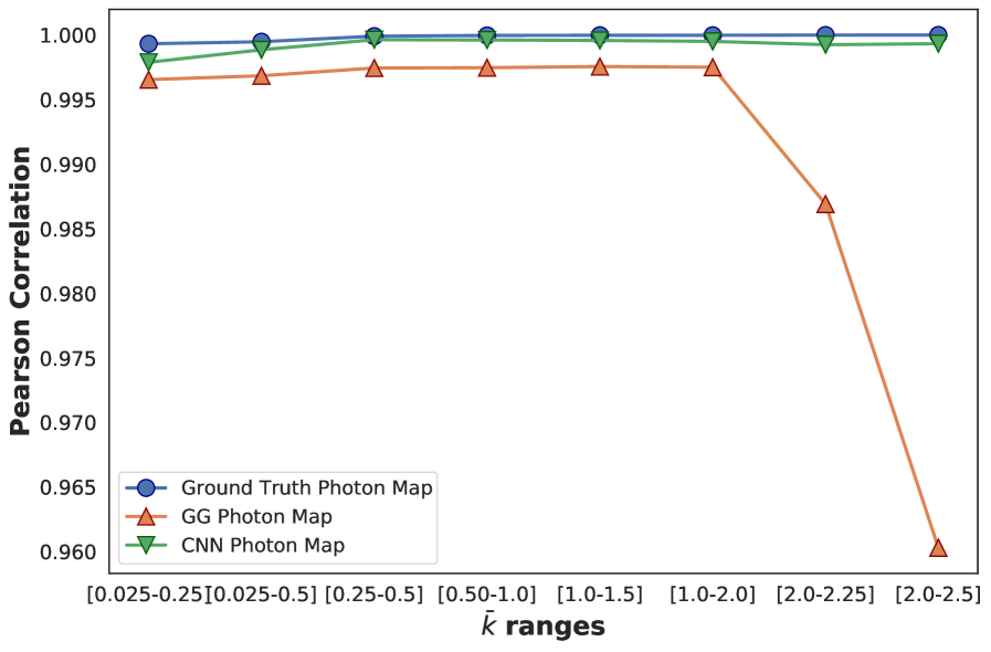
In Figure 6, we quantify the performance of the CNN model and the GGG algorithm at different ranges using the correlation in the contrast-contrast parity plot as our metric. It is evident that the GGG algorithm is slightly biased across all levels and performs poorly for . This is unsurprising, as droplet-based algorithms were designed to cope with small droplets with relatively few overlapping charge clouds. Furthermore, this implies further development of the CNN algorithm will be capable of handling large data sets.
III.3 Uncertainty Quantification
In this section, we consider a neural network ensemble approach to quantify the uncertainty in the predicted photon maps and contrasts. The motivation for such an analysis is that, while deep learning models have exhibited significant successes in their application to scientific problems, they have a tendency to engender overconfident predictions that may be inexact. As an example, neural networks are unable to recognize Out Of Distribution (OOD) instances and habitually make erroneous predictions for such cases with high confidence Amodei et al. (2016); Nguyen, Yosinski, and Clune (2015); Hendrycks and Gimpel (2016). In reliability-critical tasks, such errors and uncertainties in model predictions have led to undesirable outcomes (2016) (NTSB); (2020) (NTSB); (2017) (NTSB). In this context, quantifying the uncertainties in deep learning model predictions is highly desirable.
There are two sources of predictive uncertainty that need to be considered: Epistemic and Aleatoric. Epistemic uncertainty Smith (2013) (reducible or subjective uncertainty) arises due to lack of knowledge regarding the dynamics of the system under consideration, or an inability to express the underlying dynamics accurately using models. Epistemic uncertainties can lead to biases in the predictions. Aleatoric uncertainty Smith (2013) (irreducible uncertainty or stochastic uncertainty) arises due to noise in the training data, projection of data onto a lower space, absence of important features, etc. Aleatoric sources can lead to variances in the predictions.
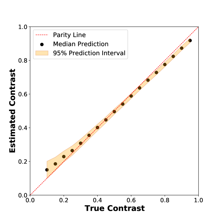
For our analysis, we use an ensemble of neural networks to make a point prediction of the contrast as well as to give an estimate of statistical uncertainty. This is in line with model ensembling based uncertainty quantification (UQ) methods validated in literature Heskes (1996); Efron (1992). Such ensembling accounts for aleatoric uncertainties due to the data and weight uncertainties. In our investigation, the neural network ensemble is formed via sequential sampling, wherein ten partially decorrelated models were sampled during the model training. Contiguous samples were spaced by ten optimization epochs each. The contrast is calculated for each model via a maximum likelihood procedure and the contrast point prediction is taken as the median predicted value. To estimate the model uncertainty, we provide a contrast prediction interval using the standard deviation of the predicted contrasts and making the assuming that the predictive distribution follows a -distribution with nine degrees of freedom (Figure 7).
We see that the error bars are larger at lower contrasts and correctly captures the notion that the prediction task is harder at lower contrasts Burdet et al. (2021b). We also notice a systematic bias in the CNN models at high contrasts. This bias may arise due to the epistemic uncertainties due to the model form (structural uncertainty). Such structural uncertainties in deep learning models cannot be accounted for by any extant approach, including the procedure used in this investigation. However, this indicates a need for more refinement on the present approach (for instance, more fine grained optimization of the model architecture, etc) and will be explored more fully in future work.
Another interesting avenue is to look at the median predicted photon map and the predicted standard deviation map to examine where the neural networks lack consensus. An example of this pair of outputs are shown in Figure 8. Evidently, the ensemble predicts insignificant uncertainty for the majority of the image with the exception of a few pixels with relatively high uncertainty. An interesting future strategy could involve using the CNN model as a fast, initial approach and subsequently run more complex fitting algorithms on regions of the image with high predicted uncertainty.
IV Conclusions
In this work, we have developed a convolutional neural network architecture which is capable of analysing single-photon X-ray speckle data in non-optimal situations, such as for small pixel size detector or with soft x-ray energies. We have benchmarked this algorithm on realistic simulated data and found that it outperforms the conventional Gaussian Greedy Guess (GGG) droplet algorithm in terms of speed and computational complexity. Furthermore, the algorithm is able to extract the contrast information for new ranges that were previously inaccessible, such as low contrast – relevant for systems which scatter weakly, as well as in a high regime. Both of the latter developments will create new opportunities to study fluctuations using XPFS in novel systems, such as in quantum or topological materials.
Acknowledgements.
This work is supported by the U.S. Department of Energy, Office of Science, Basic Energy Sciences under Award No. DE-SC0022216, as well as under Contract DE-AC02-76SF00515 for the Materials Sciences and Engineering Division. The use of the Linac Coherent Light Source (LCLS), SLAC National Accelerator Laboratory, is also supported by the DOE, Office of Science under contract DE-AC02-76SF00515. This work was also supported in part by funding from Zoox, Inc. J. J. Turner acknowledges support from the U.S. DOE, Office of Science, Basic Energy Sciences through the Early Career Research Program.Permissions
The following article has been submitted to Structural Dynamics.
Data Availability
The dataChitturi et al. (2022) that support the findings of this study are openly available at
https://doi.org/10.5281/zenodo.6643622. Machine learning models are available at https://github.com/src47/CNN_XPFS upon manuscript acceptance.
Conflict of Interest
The authors have no conflicts to disclose.
Appendix A Model Validation Metric
In this analysis, we use the average correlation (across datasets with different average count-rates) of the contrast-contrast parity model as a metric for model validation. This metric can be visualized in Figure 9.
Appendix B Value of High
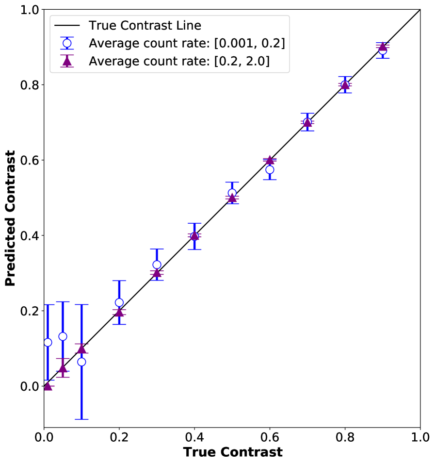
Here, we consider the value of utilizing data at higher in the fitting process. In this scenario, the photon maps are perfect samples from the negative binomial distribution (no error from the detector image to photon map conversion). At higher , high-count photon events are more probable and contain more information about the underlying distribution relative to common events (e.g. 0 or 1 photon events). It follows naturally that incorporating higher data allows for fitting the distribution with less data and more accuracy relative to only low fits. In Figure 10, we show the results of fitting the negative binomial distribution with varying uniformly in two ranges, [0.001, 0.2] and [0.2, 2.0] for 1000 datapoints. We see that at higher , the error-bars in the contrast are much smaller relative low .
References
- Decking et al. (2020) W. Decking et al., “A mhz-repetition-rate hard x-ray free-electron laser driven by a superconducting linear accelerator,” Nature Photonics 14, 391–397 (2020).
- Prat et al. (2020) E. Prat, R. Abela, M. Aiba, A. Alarcon, J. Alex, Y. Arbelo, C. Arrell, V. Arsov, C. Bacellar, C. Beard, et al., “A compact and cost-effective hard x-ray free-electron laser driven by a high-brightness and low-energy electron beam,” Nature Photonics 14, 748–754 (2020).
- Kang et al. (2017) H.-S. Kang, C.-K. Min, H. Heo, C. Kim, H. Yang, G. Kim, I. Nam, S. Y. Baek, H.-J. Choi, G. Mun, et al., “Hard x-ray free-electron laser with femtosecond-scale timing jitter,” Nature Photonics 11, 708–713 (2017).
- Ishikawa et al. (2012) T. Ishikawa, H. Aoyagi, T. Asaka, Y. Asano, N. Azumi, T. Bizen, H. Ego, K. Fukami, T. Fukui, Y. Furukawa, et al., “A compact x-ray free-electron laser emitting in the sub-ångström region,” nature photonics 6, 540–544 (2012).
- Emma et al. (2010) P. Emma, R. Akre, J. Arthur, R. Bionta, C. Bostedt, J. Bozek, A. Brachmann, P. Bucksbaum, R. Coffee, F. J. Decker, et al., “First lasing and operation of an angstrom-wavelength free-electron laser,” Nat. Photonics 4, 641–647 (2010).
- Bostedt et al. (2016) C. Bostedt, S. Boutet, D. M. Fritz, Z. Huang, H. J. Lee, H. T. Lemke, A. Robert, W. F. Schlotter, J. J. Turner, and G. J. Williams, “Linac coherent light source: The first five years,” Reviews of Modern Physics 88, 015007 (2016).
- Vinko et al. (2012) S. M. Vinko, O. Ciricosta, B. I. Cho, K. Engelhorn, H. K. Chung, C. R. Brown, T. Burian, J. Chalupsky, R. W. Falcone, C. Graves, et al., “Creation and diagnosis of a solid-density plasma with an x-ray free-electron laser,” Nature 482, 59–62 (2012).
- Bernitt et al. (2012) S. Bernitt, G. V. Brown, J. K. Rudolph, R. Steinbrugge, A. Graf, M. Leutenegger, S. W. Epp, S. Eberle, K. Kubicek, V. Mackel, et al., “An unexpectedly low oscillator strength as the origin of the fe xvii emission problem,” Nature 492, 225–228 (2012).
- Redecke et al. (2013) L. Redecke, K. Nass, D. P. DePonte, T. A. White, D. Rehders, A. Barty, F. Stellato, M. N. Liang, T. R. M. Barends, S. Boutet, et al., “Natively inhibited trypanosoma brucei cathepsin b structure determined by using an x-ray laser,” Science 339, 227–230 (2013).
- Wernet et al. (2015) P. Wernet, K. Kunnus, I. Josefsson, I. Rajkovic, W. Quevedo, M. Beye, S. Schreck, S. Grübel, M. Scholz, D. Nordlund, et al., “Orbital-specific mapping of the ligand exchange dynamics of Fe(CO)5 in solution,” Nature 520, 78–81 (2015).
- Lee et al. (2021) J.-W. Lee, M. Kim, G. Kang, S. M. Vinko, L. Bae, M. S. Cho, H.-K. Chung, M. Kim, S. Kwon, G. Lee, C. H. Nam, S. H. Park, J. H. Sohn, S. H. Yang, U. Zastrau, and B. I. Cho, “Investigation of nonequilibrium electronic dynamics of warm dense copper with femtosecond x-ray absorption spectroscopy,” Phys. Rev. Lett. 127, 175003 (2021).
- Wandel et al. (2022) S. Wandel, F. Boschini, E. H. da Silva Neto, L. Shen, M. X. Na, S. Zohar, Y. Wang, S. B. Welch, M. H. Seaberg, J. D. Koralek, G. L. Dakovski, W. Hettel, M.-F. Lin, S. P. Moeller, W. F. Schlotter, A. H. Reid, M. P. Minitti, T. Boyle, F. He, R. Sutarto, R. Liang, D. Bonn, W. Hardy, R. A. Kaindl, D. G. Hawthorn, J.-S. Lee, A. F. Kemper, A. Damascelli, C. Giannetti, J. J. Turner, and G. Coslovich, “Enhanced charge density wave coherence in a light-quenched, high-temperature superconductor,” Science 376, 860–864 (2022), https://www.science.org/doi/pdf/10.1126/science.abd7213 .
- Ament et al. (2011) L. J. P. Ament, M. van Veenendaal, T. P. Devereaux, J. P. Hill, and J. van den Brink, “Resonant inelastic x-ray scattering studies of elementary excitations,” Rev. Mod. Phys. 83, 705 (2011).
- Siefermann et al. (2014) K. R. Siefermann, C. D. Pemmaraju, S. Neppl, A. Shavorskiy, A. A. Cordones, J. Vura-Weis, D. S. Slaughter, F. P. Sturm, F. Weise, et al., “Atomic-scale perspective of ultrafast charge transfer at a dye–semiconductor interface,” The Journal of Physical Chemistry Letters 5, 2753–2759 (2014), http://dx.doi.org/10.1021/jz501264x .
- Sutton (2008) M. Sutton, “A review of x-ray intensity fluctuation spectroscopy,” C. R. Physique 9, 657 (2008).
- Shpyrko et al. (2007) O. G. Shpyrko, E. D. Isaacs, J. M. Logan, Y. Feng, G. Aeppli, R. Jaramillo, H. C. Kim, T. F. Rosenbaum, P. Zschack, M. Sprung, S. Narayanan, and A. R. Sandy, “Direct measurement of antiferromagnetic domain fluctuations,” Nature 447, 68–71 (2007).
- Sun et al. (2019) Y. Sun, N. Wang, S. Song, P. Sun, M. Chollet, T. Sato, T. B. van Driel, S. Nelson, R. Plumley, J. Montana-Lopez, S. W. Teitelbaum, J. Haber, J. B. Hastings, A. Q. R. Baron, M. Sutton, P. H. Fuoss, A. Robert, and D. Zhu, “Compact hard x-ray split-delay system based on variable-gap channel-cut crystals,” Opt. Lett. 44, 2582–2585 (2019).
- Decker et al. (2022) F.-J. Decker, K. L. Bane, W. Colocho, S. Gilevich, A. Marinelli, J. C. Sheppard, J. L. Turner, J. J. Turner, A. Vetter, S. L. Halavanau, C. Pellegrini, and A. A. Lutman, “Tunable x-ray free electron laser multi-pulses with nanosecond separation,” Scientific Reports 12, 3253 (2022).
- Shen et al. (2021) L. Shen, ·. M. Seaberg, ·. E. Blackburn, and ·. J. J. Turner, “A snapshot review-Fluctuations in quantum materials: from skyrmions to superconductivity,” MRS Advances 6, 221–233 (2021).
- Gutt et al. (2009) C. Gutt, L. M. Stadler, A. Duri, T. Autenrieth, O. Leupold, Y. Chushkin, and G. Grübel, “Measuring temporal speckle correlations at ultrafast x-ray sources,” Opt. Express 17, 55–61 (2009).
- Goodman (2007) J. Goodman, Speckle Phenomena in Optics: Theory and Applications (Roberts & Company, 2007).
- Decaro et al. (2014) C. Decaro, V. Karunaratne, S. Bera, L. Lurio, A. Sandy, S. Narayanan, M. Sutton, J. Winans, K. Duffin, J. Lehuta, and N. Karonis, “X-ray speckle visibility spectroscopy in the single-photon limit,” J. Syncrh. Rad. 20, 332 (2014).
- Bandyopadhyay et al. (2005) R. Bandyopadhyay, A. S. Gittings, S. S. Suh, P. K. Dixon, and D. J. Durian, “Speckle-visibility spectroscopy: A tool to study time-varying dynamics,” Review of Scientific Instruments 76, 093110 (2005), https://doi.org/10.1063/1.2037987 .
- Hruszkewycz et al. (2012) S. O. Hruszkewycz, M. Sutton, P. H. Fuoss, B. Adams, S. Rosenkranz, J. Ludwig, K. F., W. Roseker, D. Fritz, M. Cammarata, D. Zhu, et al., “High contrast x-ray speckle from atomic-scale order in liquids and glasses,” Phys. Rev. Lett. 109, 185502 (2012).
- Sikorski et al. (2016) M. Sikorski, Y. Feng, S. Song, D. Zhu, G. Carini, S. Herrmann, K. Nishimura, P. Hart, and A. Robert, “Application of an epix100 detector for coherent scattering using a hard x-ray free-electron laser,” Journal of Synchrotron Radiation 23, 1171–1179 (2016), https://onlinelibrary.wiley.com/doi/pdf/10.1107/S1600577516010869 .
- Sun et al. (2020) Y. Sun, J. Montana-Lopez, P. Fuoss, M. Sutton, and D. Zhu, “Accurate contrast determination for X-ray speckle visibility spectroscopy,” Journal of Synchrotron Radiation 27, 999–1007 (2020).
- Burdet et al. (2021a) N. G. Burdet, V. Esposito, M. Seaberg, C. H. Yoon, and J. Turner, “Absolute contrast estimation for soft x-ray photon fluctuation spectroscopy using a variational droplet model,” Scientific Reports 11, 1–9 (2021a).
- Campbell et al. (2021) S. I. Campbell, D. B. Allan, A. M. Barbour, D. Olds, M. S. Rakitin, R. Smith, and S. B. Wilkins, “Outlook for artificial intelligence and machine learning at the nsls-ii,” Machine Learning: Science and Technology 2, 013001 (2021).
- Konstantinova et al. (2022) T. Konstantinova, L. Wiegart, M. Rakitin, A. M. DeGennaro, and A. M. Barbour, “Machine learning enhances algorithms for quantifying non-equilibrium dynamics in correlation spectroscopy experiments to reach frame-rate-limited time resolution,” arXiv preprint arXiv:2201.07889 (2022).
- Konstantinova et al. (2021) T. Konstantinova, L. Wiegart, M. Rakitin, A. M. DeGennaro, and A. M. Barbour, “Noise reduction in x-ray photon correlation spectroscopy with convolutional neural networks encoder–decoder models,” Scientific Reports 11, 1–12 (2021).
- Blaj, Chang, and Kenney (2019) G. Blaj, C.-E. Chang, and C. J. Kenney, “Ultrafast processing of pixel detector data with machine learning frameworks,” in AIP Conference Proceedings, Vol. 2054 (AIP Publishing LLC, 2019) p. 060077.
- Blaj et al. (2017) G. Blaj, C. Kenney, J. Segal, and G. Haller, “Analytical solutions of transient drift-diffusion in pn junction pixel sensors,” arXiv preprint arXiv:1706.01429 (2017).
- Abarbanel (2019) D. Abarbanel, Artificial neural networks for analysis of coherent X-ray diffraction images (McGill University (Canada), 2019).
- Long, Shelhamer, and Darrell (2015) J. Long, E. Shelhamer, and T. Darrell, “Fully convolutional networks for semantic segmentation,” in Proceedings of the IEEE conference on computer vision and pattern recognition (2015) pp. 3431–3440.
- Seaberg et al. (2017) M. H. Seaberg, B. Holladay, J. C. T. Lee, M. Sikorski, A. H. Reid, S. A. Montoya, G. L. Dakovski, J. D. Koralek, G. Coslovich, S. Moeller, W. F. Schlotter, R. Streubel, S. D. Kevan, P. Fischer, E. E. Fullerton, J. L. Turner, F.-J. Decker, S. K. Sinha, S. Roy, and J. J. Turner, “Nanosecond x-ray photon correlation spectroscopy on magnetic skyrmions,” Phys. Rev. Lett. 119, 067403 (2017).
- Ronneberger, Fischer, and Brox (2015) O. Ronneberger, P. Fischer, and T. Brox, “U-net: Convolutional networks for biomedical image segmentation,” in International Conference on Medical image computing and computer-assisted intervention (Springer, 2015) pp. 234–241.
- Ioffe and Szegedy (2015) S. Ioffe and C. Szegedy, “Batch normalization: Accelerating deep network training by reducing internal covariate shift,” in International conference on machine learning (PMLR, 2015) pp. 448–456.
- LeNail (2019) A. LeNail, “Nn-svg: Publication-ready neural network architecture schematics.” J. Open Source Softw. 4, 747 (2019).
- Kingma and Ba (2014) D. P. Kingma and J. Ba, “Adam: A method for stochastic optimization,” arXiv preprint arXiv:1412.6980 (2014).
- Chollet et al. (2015) F. Chollet et al., “Keras,” https://keras.io (2015).
- Luque et al. (2019) A. Luque, A. Carrasco, A. Martín, and A. de Las Heras, “The impact of class imbalance in classification performance metrics based on the binary confusion matrix,” Pattern Recognition 91, 216–231 (2019).
- Herlocker et al. (2004) J. L. Herlocker, J. A. Konstan, L. G. Terveen, and J. T. Riedl, “Evaluating collaborative filtering recommender systems,” ACM Transactions on Information Systems (TOIS) 22, 5–53 (2004).
- Roseker et al. (2018) W. Roseker, S. Hruszkewycz, F. Lehmkühler, M. Walther, H. Schulte-Schrepping, S. Lee, T. Osaka, L. Strüder, R. Hartmann, M. Sikorski, et al., “Towards ultrafast dynamics with split-pulse x-ray photon correlation spectroscopy at free electron laser sources,” Nature communications 9, 1–6 (2018).
- Burdet et al. (2021b) N. G. Burdet, V. Esposito, M. H. Seaberg, C. H. Yoon, and J. J. Turner, “Absolute contrast estimation for soft X-ray photon fluctuation spectroscopy using a variational droplet model,” Scientific Reports 11, 1–9 (2021b).
- Kirk and Wen-Mei (2016) D. B. Kirk and W. H. Wen-Mei, Programming massively parallel processors: a hands-on approach (Morgan kaufmann, 2016).
- Amodei et al. (2016) D. Amodei, C. Olah, J. Steinhardt, P. Christiano, J. Schulman, and D. Mané, “Concrete problems in ai safety,” arXiv preprint arXiv:1606.06565 (2016).
- Nguyen, Yosinski, and Clune (2015) A. Nguyen, J. Yosinski, and J. Clune, “Deep neural networks are easily fooled: High confidence predictions for unrecognizable images,” in Proceedings of the IEEE conference on computer vision and pattern recognition (2015) pp. 427–436.
- Hendrycks and Gimpel (2016) D. Hendrycks and K. Gimpel, “A baseline for detecting misclassified and out-of-distribution examples in neural networks,” arXiv preprint arXiv:1610.02136 (2016).
- (49) N. T. S. B. (NTSB), “Collision between a Car Operating with Automated Vehicle Control Systems and a Tractor-Semitrailer Truck, NTSB/HAR-17-XX,” Tech. Rep. (NATIONAL TRANSPORTATION SAFETY BOARD, 2016).
- (50) N. T. S. B. (NTSB), “Collision Between a Sport Utility Vehicle Operating With Partial Driving Automation and a Crash Attenuator, NTSB/HAR-20/01,” Tech. Rep. (NATIONAL TRANSPORTATION SAFETY BOARD, 2020).
- (51) N. T. S. B. (NTSB), “Collision Between a Car Operating With Automated Vehicle Control Systems and a Tractor-Semitrailer Truck,NTSB/HAR-17/02,” Tech. Rep. (NATIONAL TRANSPORTATION SAFETY BOARD, 2017).
- Smith (2013) R. C. Smith, Uncertainty quantification: theory, implementation, and applications, Vol. 12 (SIAM, 2013).
- Heskes (1996) T. Heskes, “Practical confidence and prediction intervals,” Advances in neural information processing systems 9 (1996).
- Efron (1992) B. Efron, “Bootstrap methods: another look at the jackknife,” in Breakthroughs in statistics (Springer, 1992) pp. 569–593.
- Chitturi et al. (2022) S. Chitturi, N. Burdet, Y. Nashed, D. Ratner, A. Mishra, T. Lane, M. Seaberg, V. Esposito, C. H. Yoon, M. Dunne, and J. Turner, “Simulated x-ray photon fluctuation spectroscopy dataset,” Zenodo (2022), 10.5281/zenodo.6643622.