A majorized PAM method with subspace correction for low-rank composite factorization model

Ting Tao¹¹1(taoting@fosu.edu.cn) School of Mathematics, Foshan University, Foshan Yitian Qian²²2(yitian.qian@polyu.edu.hk) Department of Applied Mathematics, The Hong Kong Polytechnic University, Hong Kong and Shaohua Pan³³3(shhpan@scut.edu.cn) School of Mathematics, South China University of Technology, Guangzhou

Abstract

This paper concerns a class of low-rank composite factorization models arising from matrix completion. For this nonconvex and nonsmooth optimization problem, we propose a proximal alternating minimization algorithm (PAMA) with subspace correction, in which a subspace correction step is imposed on every proximal subproblem so as to guarantee that the corrected proximal subproblem has a closed-form solution. For this subspace correction PAMA, we prove the subsequence convergence of the iterate sequence, and establish the convergence of the whole iterate sequence and the column subspace sequences of factor pairs under the KL property of objective function and a restrictive condition that holds automatically for the column $\ell_{2,0}$ -norm function. Numerical comparison with the proximal alternating linearized minimization method on one-bit matrix completion problems indicates that PAMA has an advantage in seeking lower relative error within less time.

keywords Low-rank factor model; alternating minimization method; subspace correction; global convergence

1 Introduction

Let $\mathbb{R}^{n\times m}\ (n\leq m)$ be the space of all $n\times m$ real matrices, equipped with the trace inner product $\langle\cdot,\cdot\rangle$ and its induced Frobenius norm $\|\cdot\|_{F}$ . Fix any $r\in\{1,\ldots,n\}$ and write $\mathbb{X}_{r}\!:=\mathbb{R}^{n\times r}\times\mathbb{R}^{m\times r}$ . We are interested in the low-rank composite factorization model

\min_{(U,V)\in\mathbb{X}_{r}}\Phi_{\lambda,\mu}(U,V):=f(UV^{\top})+\lambda\sum_{i=1}^{r}\big{[}\theta(\|U_{i}\|)+\theta(\|V_{i}\|)\big{]}+\frac{\mu}{2}\big{[}\|U\|_{F}^{2}+\|V\|_{F}^{2}\big{]},

(1)

where $f\!:\mathbb{R}^{n\times m}\to\mathbb{R}$ is a lower bounded $L_{\!f}$ -smooth (i.e., $f$ is continuously differentiable and its gradient $\nabla\!f$ is Lipschitz continuous with modulus $L_{f}$ ) function, $\|U_{i}\|$ and $\|V_{i}\|$ denote the Euclidean norm of the $i$ th column of $U$ and $V$ , $\lambda>0$ is a regularization parameter, $\mu>0$ is a small constant, and $\theta\!:\mathbb{R}\to\overline{\mathbb{R}}:=(-\infty,\infty]$ is a proper lower semicontinuous (lsc) function to promote sparsity and satisfy the following two conditions:

(C.1): $\theta(0)=0$ , $\theta(t)>0$ for $t>0$ , and $\theta(t)=\infty$ for $t<0$ ;
(C.2): $\theta$ is differentiable on $\mathbb{R}_{++}$ , and its proximal mapping has a closed-form.

Model (1) has a wide application in matrix completion and sensing (see, e.g., [3, 6, 14, 8]). Among others, the term $\frac{\mu}{2}(\|U\|_{F}^{2}+\|V\|_{F}^{2})$ plays a twofold role: one is to ensure that (1) has a nonempty set of optimal solutions and then a nonempty set of stationary points, and the other is to guarantee that (1) has a balanced set of stationary points (see Proposition 1). The regularization term $\lambda\big{[}\sum_{i=1}^{r}\theta(\|U_{i}\|)+\theta(\|V_{i}\|)\big{]}$ aims at promoting low-rank solutions via column sparsity of factors $U$ and $V$ . Table 1 below provides some examples of $\theta$ to satisfy conditions (C.1)-(C.2), where $\theta_{4}$ and $\theta_{5}$ satisfy (C.2) by [9, 26]. When $\theta=\theta_{1}$ , model (1) is the column $\ell_{2,0}$ -norm regularization problem studied in [24], and when $\theta=\theta_{2}$ , it becomes the factorized form of the nuclear-norm regularization problem [15, 18]. In the sequel, we write

F(U,V)\!:=f(UV^{\top})\ \ {\rm for}\ (U,V)\in\mathbb{X}_{r}\ \ {\rm and}\ \ \vartheta(W)\!:={\textstyle\sum_{i=1}^{r}}\theta(\|W_{i}\|)\ \ {\rm for}\ W\!\in\mathbb{R}^{l\times r}.

(2)

Table 1: Some common functions satisfying conditions (C.1)-(C.2)

$\theta_{1}(t)=\left\{\begin{array}[]{cl}{\rm sign}(t)&{\rm if}\ t\in\mathbb{R}_{+},\\ \infty&{\rm otherwise}\end{array}\right.$	$\theta_{2}(t)=\left\{\begin{array}[]{cl}t^{2}&{\rm if}\ t\in\mathbb{R}_{+},\\ \infty&{\rm otherwise}\end{array}\right.$
$\theta_{3}(t)=\left\{\begin{array}[]{cl}t&{\rm if}\ t\in\mathbb{R}_{+},\\ \infty&{\rm otherwise}\end{array}\right.$	$\theta_{4}(t)=\left\{\begin{array}[]{cl}t^{1/2}&{\rm if}\ t\in\mathbb{R}_{+},\\ \infty&{\rm otherwise}\end{array}\right.$
$\theta_{5}(t)=\left\{\begin{array}[]{cl}t^{2/3}&{\rm if}\ t\in\mathbb{R}_{+},\\ \infty&{\rm otherwise}\end{array}\right.$	$\theta_{6}(t)=\!\left\{\begin{array}[]{cl}1&\textrm{if}\ t>\frac{2a}{\rho(a+1)},\\ \!\rho t-\!\frac{(\rho(a+1)t-2)^{2}}{4(a^{2}-1)}&{\rm if}\ \frac{2}{\rho(a+1)}<t\leq\frac{2a}{\rho(a+1)},\\ \rho t&{\rm if}\ 0\leq t\leq\frac{2}{a+1},\\ \infty&{\rm if}\ t<0\\ \end{array}\right.\ \ (a>1)$

1.1 Related work

Problem (1) is a special case of the optimization models considered in [1, 2, 10, 16, 17, 25], for which the nonsmooth regularization term has a separable structure and the nonsmooth function associated with each block has a closed-form proximal mapping. Hence, the proximal alternating linearized minimization (PALM) methods and their inertial versions developed in [1, 2, 17, 25] are suitable for dealing with (1), whose basic idea is to minimize alternately a proximal version of the linearization of $\Phi_{\lambda,\mu}$ at the current iterate, the sum of the linearization of $F$ at this iterate and $\lambda\sum_{i=1}^{r}\!\big{[}\theta(\|U_{i}\|)+\theta(\|V_{i}\|)\big{]}+\frac{\mu}{2}\big{[}\|U\|_{F}^{2}+\|V\|_{F}^{2}\big{]}$ . The iteration of these PALM methods depends on the global Lipschitz moduli $L_{1}(V^{\prime})$ and $L_{1}(U^{\prime})$ of the partial gradients $\nabla_{U}F(\cdot,V^{\prime})$ and $\nabla_{V}F(U^{\prime},\cdot)$ for any fixed $V^{\prime}\!\in\mathbb{R}^{m\times r}$ and $U^{\prime}\in\mathbb{R}^{n\times r}$ . These constants are available whenever that of $\nabla\!f$ is known, but they are usually much larger than that of $\nabla\!f$ , which brings a challenge to the solution of subproblems with a first-order method. Although the descent lemma can be employed to search a tighter one in computation, it is consuming due to solution of additional subproblems. Since the Lipschitz constant of $\nabla\!f$ is available or easier to estimate, it is natural to ask whether an efficient alternating minimization (AM) method can be designed by using the Lipschitz continuity of $\nabla\!f$ only. The block coordinate variable metric algorithms in [10, 16] are also applicable to (1), but their efficiency is dependent on an appropriate choice of variable metric linear operators, and their convergence analysis requires the exact solutions of variable metric subproblems. Now it is unclear which kind of variable metric linear operators is suitable for (1), and whether the variable metric subproblems involving nonsmooth $\vartheta$ have a closed-form solution.

Recently, the authors tried an AM method for problem (1) with $\theta=\theta_{1}$ by leveraging the Lipschitz continuity of $\nabla\!f$ only (see [24, Algorithm 2]), tested its efficiency on matrix completion problems with $f(X)=\frac{1}{2}\|X\|_{F}^{2}$ for $X\in\mathbb{R}^{n\times m}$ , but did not achieve any convergence results on the generated iterate sequence [24]. This work is a deep dive of [24] and aims to provide a convergence certificate for the iterate sequence of this AM method.

1.2 Main contribution

We achieve a majorization of $\Phi_{\lambda,\mu}$ at each iterate by using the Lipschitz continuity of $\nabla\!f$ , and propose a proximal AM method by minimizing this majorization alternately, which is an extension of the proximal AM algorithm of [24] to the general model (1). The main contributions of this work involve the following three aspects.

(i) The proposed PAMA only involves the Lipschitz constant of $\nabla\!f$ , which is usually known or easier to estimate before starting algorithm. Then, compared with the existing PALM methods and their inertial versions in [1, 2, 17, 25], this PAMA has a potential advantage in running time due to avoiding the estimation of $L_{1}(V^{\prime})$ and $L_{1}(U^{\prime})$ in each iteration.

(ii) As will be shown in Section 3, our PAMA is actually a variable metric proximal AM method. Different from the variable metric methods in [10, 16], our variable metric linear operators are natural products of majorizing $F$ by the Lipschitz continuity of $\nabla\!f$ . In particular, by introducing a subspace correction step to per subproblem, we overcome the difficulty that the variable metric proximal subproblems involving $\vartheta$ have no closed-form solutions.

(iii) Our majorized PAMA with subspace correction has a theoretical certificate. Specifically, we prove the subsequence convergence of the iterate sequence for all $\theta_{i}$ in Table 1, and establish the convergence of the whole iterate sequence and the column subspace sequences of factor pairs under the KL property of $\Phi_{\lambda,\mu}$ and the restrictive conditions (29a)-(29b) that can be satisfied by $\theta_{1}$ , or by $\theta_{4}$ - $\theta_{5}$ if there is a stationary point with distinct nonzero singular values. To the best of our knowledge, this appears to be the first subspace correction AM method with convergence certificate for low-rank composite factorization models. Hastie et al. [13] proposed a PAMA with subspace correction (named softImpute-ALS) for the factorization form of the nuclear-norm regularized least squares model, but did not provide the convergence analysis of the iterate sequence even the objective value sequence.

1.3 Notation

Throughout this paper, $I_{r}$ means a $r\times r$ identity matrix, $\mathbb{O}^{n_{1}\times n_{2}}$ denotes the set of all $n_{1}\times n_{2}$ matrices with orthonormal columns, and $\mathbb{O}^{n_{1}}$ means $\mathbb{O}^{n_{1}\times n_{1}}$ . For a matrix $X\in\mathbb{R}^{n_{1}\times n_{2}}$ , $\|X\|,\,\|X\|_{*}$ and $\|X\|_{2,0}$ denote the spectral norm, nuclear norm, and column $\ell_{2,0}$ -norm of $X$ , respectively, $\sigma(X)=(\sigma_{1}(X),\ldots,\sigma_{n}(X))^{\top}$ with $\sigma_{1}(X)\geq\cdots\geq\sigma_{n}(X)$ , $\mathbb{O}^{n,m}(X)\!:=\{(U,V)\in\mathbb{O}^{n}\times\mathbb{O}^{m}\ |\ X=U[{\rm Diag}(\sigma(X))\ \ 0]V^{\top}\}$ , and $\Sigma_{\kappa}(X)={\rm Diag}(\sigma_{1}(x),\ldots,\sigma_{\kappa}(X))$ . For an integer $k\geq 1$ , $[k]\!:=\{1,\ldots,k\}$ . For a matrix $Z\in\mathbb{R}^{n_{1}\times n_{2}}$ , $Z_{j}$ means the $j$ th column of $Z$ , $J_{Z}$ denotes its index set of nonzero columns, ${\rm col}(Z)$ and ${\rm row}(Z)$ denote the subspace spanned by all columns and rows of $Z$ . For an index set $J\subset[r]$ , we write $\overline{J}:=[r]\backslash J$ , and define

\vartheta_{\!J}(Z_{J})={\textstyle\sum_{i\in J}}\,\theta(\|Z_{i}\|)\ \ {\rm and}\ \vartheta_{\overline{J}}(Z_{\overline{J}})={\textstyle\sum_{i\in\overline{J}}}\,\theta(\|Z_{i}\|)\ \ {\rm for}\ Z\in\mathbb{R}^{l\times r}.

(3)

2 Preliminaries

Recall that for a proper lsc function $h\!:\mathbb{R}^{n}\to\overline{\mathbb{R}}$ , its proximal mapping associated with parameter $\gamma>0$ is defined as $\mathcal{P}_{\!\gamma}h(z):=\mathop{\arg\min}_{x\in\mathbb{R}^{n}}\big{\{}\frac{1}{2\gamma}\|z-x\|^{2}+h(x)\big{\}}$ for $z\in\mathbb{R}^{n}$ . The mapping $\mathcal{P}_{\!\gamma}h$ is generally multi-valued unless the function $h$ is convex. The following lemma states that the proximal mapping of the function $\vartheta$ in (2) can be obtained with that of $\theta$ . Since its proof is immediate by condition (C.1), we do not include it.

Lemma 2.1

Fix any $\gamma>0$ and $u\in\mathbb{R}^{n}$ . Let $S^{*}$ be the optimal solution set of

\min_{x\in\mathbb{R}^{n}}\Big{\{}\frac{1}{2}\|\gamma x-u\|^{2}+\lambda\theta(\|x\|)\Big{\}}.

Then, $S^{*}=\{0\}$ when $u=0$ ; otherwise $S^{*}=\frac{u}{\|u\|}\mathcal{P}_{\!\lambda/\gamma^{2}}\theta(\|u\|/\gamma)$ .

2.1 Stationary point of problem (1)

Before introducing the concept of stationary points for problem (1), we first recall from [19] the notion of subdifferentials.

Definition 2.1

Consider a function $h\!:\mathbb{R}^{n\times m}\to\overline{\mathbb{R}}$ and a point $x$ with $h(x)$ finite. The regular subdifferential of $h$ at $x$ , denoted by $\widehat{\partial}h(x)$ , is defined as

\widehat{\partial}h(x):=\bigg{\{}v\in\mathbb{R}^{n\times m}\ \big{|}\ \liminf_{x\neq x^{\prime}\to x}\frac{h(x^{\prime})-h(x)-\langle v,x^{\prime}-x\rangle}{\|x^{\prime}-x\|_{F}}\geq 0\bigg{\}},

and the basic (known as limiting or Morduhovich) subdifferential of $h$ at $x$ is defined as

\partial h(x):=\Big{\{}v\in\mathbb{R}^{n\times m}\ |\ \exists\,x^{k}\to x\ {\rm with}\ h(x^{k})\to h(x)\ {\rm and}\ v^{k}\to v\ {\rm with}\ v^{k}\in\widehat{\partial}h(x^{k})\Big{\}}.

The following lemma characterizes the subdifferential of the function $\vartheta$ in (2). Since the proof is immediate by [19, Theorem 10.49 & Proposition 10.5], we omit it.

Lemma 2.2

At a given $(\overline{U},\overline{V})\in\mathbb{X}_{r}$ , $\partial\vartheta(\overline{U})\!=\overline{\mathcal{U}}_{1}\times\cdots\times\overline{\mathcal{U}}_{r}$ and $\vartheta(\overline{V})\!=\overline{\mathcal{V}}_{1}\times\cdots\times\overline{\mathcal{V}}_{r}$ with

\mathcal{\overline{U}}_{j}\!=\!\left\{\begin{array}[]{cl}\Big{\{}\frac{\theta^{\prime}(\|\overline{U}_{j}\|)\overline{U}_{j}}{\|\overline{U}_{j}\|}\Big{\}}&\ {\rm if}\ \overline{U}_{j}\!\neq\!0,\\ \!\bigcup_{y\in\partial\theta(0)}\partial(y\|\cdot\|)&\ {\rm if}\ \overline{U}_{\!j}\!=\!0\end{array}\right.\ {\rm and}\ \mathcal{\overline{V}}_{j}\!=\!\left\{\begin{array}[]{cl}\Big{\{}\frac{\theta^{\prime}(\|\overline{V}_{j}\|)\overline{V}_{j}}{\|\overline{V}_{j}\|}\Big{\}}&\ {\rm if}\ \overline{V}_{j}\!\neq\!0,\\ \!\bigcup_{y\in\partial\theta(0)}\partial(y\|\cdot\|)&\ {\rm if}\ \overline{V}_{\!j}\!=\!0.\end{array}\right.

Motivated by Lemma 2.2, we introduce the following concept of stationary points.

Definition 2.2

A factor pair $(\overline{U},\overline{V})\in\mathbb{X}_{r}$ is called a stationary point of problem (1) if

0\in\partial\Phi_{\lambda,\mu}(\overline{U},\overline{V})=\begin{pmatrix}\nabla_{U}f(\overline{U}\overline{V}^{\top})\overline{V}+\mu\overline{U}+\lambda[\,\mathcal{\overline{U}}_{1}\times\cdots\times\mathcal{\overline{U}}_{r}]\\ \big{[}\nabla_{V}f(\overline{U}\overline{V}^{\top})\big{]}^{\top}\overline{U}+\mu\overline{V}+\lambda[\,\mathcal{\overline{V}}_{1}\times\cdots\times\mathcal{\overline{V}}_{r}]\end{pmatrix}

where, for each $j\in[r]$ , the sets $\mathcal{\overline{U}}_{j}$ and $\mathcal{\overline{V}}_{j}$ take the same form as in Lemma 2.2.

2.2 Relation between column $\ell_{2,p}$ -norm and Schatten $p$ -norm

Fix any $p\in(0,1]$ . Recall that the column $\ell_{2,p}$ -norm of a matrix $X\in\mathbb{R}^{n\times m}$ is defined as $\|X\|_{2,p}\!:=\big{(}\sum_{j=1}^{m}\|X_{j}\|^{p}\big{)}^{{1}/{p}}$ , while its Schatten $p$ -norm is defined as $\|X\|_{\rm S_{p}}\!:=\big{(}\sum_{i=1}^{n}[\sigma_{i}(X)]^{p}\big{)}^{{1}/{p}}$ . The following lemma states that $\|X\|_{\rm S_{p}}$ is not greater than $\ell_{2,p}$ -norm $\|X\|_{2,p}$ .

Lemma 2.3

Fix any $X\in\mathbb{R}^{n\times m}$ of rank $r$ . For any $R\in\mathbb{O}^{d\times r}$ with $r\leq d\leq n$ , it holds that $\|X\|^{p}_{\rm S_{p}}\leq\sum_{i=1}^{d}\big{[}(R\Sigma_{r}(X)R^{\top})_{ii}\big{]}^{p}$ and consequently $\|X\|^{p}_{\rm S_{p}}\leq\|X\|^{p}_{2,p}$ .

Proof: For each $i\in[d]$ , $(R\Sigma_{r}(X)R^{\top})_{ii}=\sum_{j=1}^{r}R_{ij}^{2}\sigma_{j}(X)$ , which implies that

\sum_{i=1}^{d}\big{[}(R\Sigma_{r}(X)R^{\top})_{ii}\big{]}^{p}=\sum_{i=1}^{d}\Big{(}\sum_{j=1}^{r}R_{ij}^{2}\sigma_{j}(X)\Big{)}^{p}.

For each $i\in[d]$ , let $\alpha_{i}=\sum_{j=1}^{r}R_{ij}^{2}$ . As $R\in\mathbb{O}^{d\times r}$ , we have $\alpha_{i}\in[0,1]$ for each $i\in[d]$ . Note that the function $\mathbb{R}_{+}\ni t\mapsto t^{p}$ is concave because $p\in(0,1]$ . Moreover, if $\alpha_{i}\neq 0$ , $\sum_{j=1}^{r}{R_{ij}^{2}}/{\alpha_{i}}=1$ . For each $i\in[d]$ with $\alpha_{i}\neq 0$ , from Jensen’s inequality,

\Big{(}\sum\limits_{j=1}^{r}\frac{R_{ij}^{2}}{\alpha_{i}}\sigma_{j}(X)\Big{)}^{p}\geq\sum\limits_{j=1}^{r}\frac{R_{ij}^{2}}{\alpha_{i}}(\sigma_{j}(X))^{p},

which by $\alpha_{i}\!\in\!(0,1]$ and $0\!<\!p\!\leq\!1$ implies that $\big{(}\sum_{j=1}^{r}R_{ij}^{2}\sigma_{j}(X)\big{)}^{p}\!\geq\!\sum_{j=1}^{r}R_{ij}^{2}(\sigma_{j}(X))^{p}$ . Together with $1=\sum_{i=1}^{d}R_{ij}^{2}=\sum_{i:\,\alpha_{i}\neq 0}R_{ij}^{2}$ for each $j\in[r]$ , it follows that

	$\displaystyle\sum_{i=1}^{d}\big{[}(R\Sigma_{r}(X)R^{\top})_{ii}\big{]}^{p}$	$\displaystyle=\sum_{i=1}^{d}\Big{(}\sum_{j=1}^{r}R_{ij}^{2}\sigma_{j}(X)\Big{)}^{p}=\sum_{i:\,\alpha_{i}\neq 0}\Big{(}\sum_{j=1}^{r}R_{ij}^{2}\sigma_{j}(X)\Big{)}^{p}$
		$\displaystyle\geq\sum_{i:\,\alpha_{i}\neq 0}\sum_{j=1}^{r}R_{ij}^{2}(\sigma_{j}(X))^{p}=\sum_{j=1}^{r}(\sigma_{j}(X))^{p}.$		(4)

The first part then follows. For the second part, let $X$ have the thin SVD as $X=P_{1}\Sigma_{r}(X)Q_{1}^{\top}$ with $P_{1}\in\mathbb{O}^{n\times r}$ and $Q_{1}\in\mathbb{O}^{m\times r}$ . By the definition, it holds that

\|X\|^{p}_{\rm S_{p}}\!=\!\sum_{i=1}^{r}(\sigma_{i}^{2}(X))^{p/2}\leq\sum_{i=1}^{m}\big{[}(Q_{1}\Sigma_{r}(X)^{2}Q_{1}^{\top})_{ii}\big{]}^{p/2}\!=\!\sum_{i=1}^{m}\big{[}(X^{\top}X)_{ii}\big{]}^{{p}/{2}}\!=\!\|X\|_{2,p}^{p}

where the inequality is implied by the above (2.2). The proof is completed. $\Box$

By invoking Lemma 2.3, we obtain the factorization form of the Schatten $p$ -norm.

Proposition 2.1

For any matrix $X\in\mathbb{R}^{n\times m}$ with rank $r\leq d$ , it holds that

2\|X\|_{\rm S_{p}}^{p}=\min_{U\in\mathbb{R}^{n\times d},V\in\mathbb{R}^{m\times d}}\Big{\{}\|U\|_{2,p}^{2p}+\|V\|_{2,p}^{2p}\ \ {\rm s.t.}\ \ X=UV^{\top}\Big{\}}.

Proof: From [20, Theorem 2], it follows that the following relation holds

\|X\|_{\rm S_{p}}=\min_{U\in\mathbb{R}^{n\times d},V\in\mathbb{R}^{m\times d}\atop X=UV^{\top}}\frac{1}{2^{1/p}}\Big{(}\|U\|^{2p}_{\rm S_{2p}}+\|V\|^{2p}_{\rm S_{2p}}\Big{)}^{1/p},

which together with Lemma 2.3 immediately implies that

\|X\|_{\rm S_{p}}\leq\min_{U\in\mathbb{R}^{n\times d},V\in\mathbb{R}^{m\times d}\atop X=UV^{\top}}\frac{1}{2^{1/p}}\Big{(}\|U\|^{2p}_{2,p}+\|V\|^{2p}_{2,p}\Big{)}^{1/p}.

By taking $\overline{U}=P_{1}[\Sigma_{d}(X)]^{1/2}$ and $\overline{V}=Q_{1}[\Sigma_{d}(X)]^{1/2}$ where $X=P_{1}\Sigma_{d}(X)Q_{1}^{\top}$ with $P_{1}\in\mathbb{O}^{n\times d}$ and $Q_{1}\in\mathbb{O}^{m\times d}$ is the thin SVD of $X$ , we get $\|\overline{U}\|^{2p}_{2,p}=\|\overline{V}\|^{2p}_{2,p}=\|X\|^{p}_{\rm S_{p}}$ . The result holds. $\Box$

2.3 Kurdyka-Lojasiewicz property

We recall from [1] the concept of the KL property of an extended real-valued function.

Definition 2.3

Let $h\!:\mathbb{X}\to\overline{\mathbb{R}}$ be a proper lower semicontinuous (lsc) function. The function $h$ is said to have the Kurdyka-Lojasiewicz (KL) property at $\overline{x}\in{\rm dom}\,\partial h$ if there exist $\eta\in(0,+\infty]$ , a continuous concave function $\varphi\!:[0,\eta)\to\mathbb{R}_{+}$ satisfying

(i)

$\varphi(0)=0$ and $\varphi$ is continuously differentiable on $(0,\eta)$ ,
(ii)

for all $s\in(0,\eta)$ , $\varphi^{\prime}(s)>0$ ;

and a neighborhood $\mathcal{U}$ of $\overline{x}$ such that for all $x\in\mathcal{U}\cap\big{[}h(\overline{x})<h(x)<h(\overline{x})+\eta\big{]},$

\varphi^{\prime}(h(x)-h(\overline{x})){\rm dist}(0,\partial h(x))\geq 1.

If $h$ satisfies the KL property at each point of ${\rm dom}\,\partial h$ , then it is called a KL function.

Remark 2.1

By Definition 2.3 and [1, Lemma 2.1], a proper lsc function has the KL property at every point of $(\partial h)^{-1}(0)$ . Thus, to show that a proper lsc $h\!:\mathbb{X}\to\overline{\mathbb{R}}$ is a KL function, it suffices to check that $h$ has the KL property at any critical point.

3 A majorized PAMA with subspace correction

Fix any $(U^{\prime},V^{\prime})\in\mathbb{X}_{r}$ . Recall that $\nabla f$ is Lipschitz continuous with modulus $L_{\!f}$ . Then, for any $(U,V)\in\mathbb{X}_{r}$ , it holds that

f(UV^{\top}\!)\!\leq\!f(U^{\prime}{V^{\prime}}^{\top}\!)\!+\!\langle\nabla\!f(U^{\prime}{V^{\prime}}^{\top}\!),UV^{\top}\!-\!U^{\prime}{V^{\prime}}^{\top}\rangle\!+\!\frac{L_{\!f}}{2}\|UV^{\top}\!\!-\!U^{\prime}{V^{\prime}}^{\top}\!\|_{F}^{2}:=\!\widehat{F}(U,V,U^{\prime},V^{\prime}),

(5)

which together with the expression of $\Phi_{\lambda,\mu}$ immediately implies that

\Phi_{\lambda,\mu}(U,V)\leq\widehat{F}(U,V,U^{\prime},V^{\prime})+\lambda\big{[}\vartheta(U)+\vartheta(V)\big{]}+\frac{\mu}{2}\big{(}\|U\|_{F}^{2}+\|V\|_{F}^{2}\big{)}:=\widehat{\Phi}_{\lambda,\mu}(U,V,U^{\prime},V^{\prime}).

(6)

Note that $\widehat{\Phi}_{\lambda,\mu}(U^{\prime},V^{\prime},U^{\prime},V^{\prime})=\Phi_{\lambda,\mu}(U^{\prime},V^{\prime})$ , so $\widehat{\Phi}_{\lambda,\mu}(\cdot,\cdot,U^{\prime},V^{\prime})$ is a majorization of $\Phi_{\lambda,\mu}$ at $(U^{\prime},V^{\prime})$ . Let $(U^{k},V^{k})$ be the current iterate. It is natural to develop an algorithm for problem (1) by minimizing the function $\widehat{\Phi}_{\lambda,\mu}(\cdot,\cdot,U^{k},V^{k})$ alternately or by the following iteration:

		$\displaystyle U^{k+1}\in\mathop{\arg\min}_{U\in\mathbb{R}^{n\times r}}\Big{\{}\langle\nabla_{U}\!F(U^{k},V^{k}),U\rangle+\lambda\vartheta(U)+\frac{\mu}{2}\\|U\\|_{F}^{2}\!+\!\frac{L_{f}}{2}\\|(U-U^{k})(V^{k})^{\top}\\|_{F}^{2}\Big{\}},$
		$\displaystyle V^{k+1}\in\mathop{\arg\min}_{V\in\mathbb{R}^{m\times r}}\Big{\{}\langle\nabla_{V}\!F(U^{k+1},V^{k}),V\rangle+\lambda\vartheta(V)+\frac{\mu}{2}\\|V\\|_{F}^{2}\!+\!\frac{L_{f}}{2}\\|U^{k+1}(V\!-\!V^{k})^{\top}\\|_{F}^{2}\Big{\}}.$

Compared with the PALM method, such a majorized AM method is actually a variable metric proximal AM method. Unfortunately, due to the nonsmooth regularizer $\vartheta$ , these two variable metric subproblems have no closed-form solutions, which brings a great challenge for convergence analysis of the generated iterate sequence. Inspired by the fact that variable metric proximal methods are more effective especially for ill-conditioned problems, we introduce a subspace correction step to per proximal subproblem so as to guarantee that the variable metric proximal subproblem at the corrected factor has a closed-form solution, and propose the following majorized PAMA with subspace correction.

Algorithm 1 (A majorized PAMA with subspace correction)

Initialization: Input parameters $\varrho\in(0,1),\underline{\gamma_{1}}>0,\underline{\gamma_{2}}>0,\gamma_{1,0}>0$ and $\gamma_{2,0}>0$ . Choose $\overline{P}^{0}\!\in\mathbb{O}^{m\times r},\widehat{P}^{0}\!\in\mathbb{O}^{n\times r},\overline{Q}^{0}=\overline{D}^{0}=I_{r}$ , and let $(\overline{U}^{0},\overline{V}^{0})=(\widehat{P}^{0},\overline{P}^{0})$ .
For $k=0,1,2,\ldots$ do

1.

Compute $U^{k+1}\in\displaystyle{\mathop{\arg\min}_{U\in\mathbb{R}^{n\times r}}}\Big{\{}\widehat{\Phi}_{\lambda,\mu}(U,\overline{V}^{k},\overline{U}^{k},\overline{V}^{k})+\frac{\gamma_{1,k}}{2}\|U-\overline{U}^{k}\|_{F}^{2}\Big{\}}.$

Perform a thin SVD for $U^{k+1}\overline{D}^{k}$ such that $U^{k+1}\overline{D}^{k}=\widehat{P}^{k+1}(\widehat{D}^{k+1})^{2}(\widehat{Q}^{k+1})^{\top}$ with $\widehat{P}^{k+1}\in\mathbb{O}^{n\times r},\widehat{Q}^{k+1}\in\mathbb{O}^{r}$ and $(\widehat{D}^{k+1})^{2}={\rm Diag}(\sigma(U^{k+1}\overline{D}^{k}))$ , and set

\widehat{U}^{k+1}:=\widehat{P}^{k+1}\widehat{D}^{k+1},\ \ \widehat{V}^{k+1}\!:=\overline{P}^{k}\widehat{Q}^{k+1}\widehat{D}^{k+1}\ \ {\rm and}\ \ \widehat{X}^{k+1}\!:=\widehat{U}^{k+1}(\widehat{V}^{k+1})^{\top}.

3.

Compute $V^{k+1}\in\displaystyle{\mathop{\arg\min}_{V\in\mathbb{R}^{m\times r}}}\Big{\{}\widehat{\Phi}_{\lambda,\mu}(\widehat{U}^{k+1},V,\widehat{U}^{k+1},\widehat{V}^{k+1})+\frac{\gamma_{2,k}}{2}\|V-\widehat{V}^{k+1}\|_{F}^{2}\Big{\}}.$

Find a thin SVD for $V^{k+1}\widehat{D}^{k+1}$ such that $V^{k+1}\widehat{D}^{k+1}=\overline{P}^{k+1}(\overline{D}^{k+1})^{2}(\overline{Q}^{k+1})^{\top}$ with $\overline{P}^{k+1}\in\mathbb{O}^{m\times r},\overline{Q}^{k+1}\in\mathbb{O}^{r}$ and $(\overline{D}^{k+1})^{2}={\rm Diag}(\sigma(V^{k+1}\widehat{D}^{k+1}))$ , and set

\overline{U}^{k+1}\!:=\widehat{P}^{k+1}\overline{Q}^{k+1}\overline{D}^{k+1},\ \ \overline{V}^{k+1}\!:=\overline{P}^{k+1}\overline{D}^{k+1}\ \ {\rm and}\ \ \overline{X}^{k+1}\!:=\overline{U}^{k+1}(\overline{V}^{k+1})^{\top}\!.

5.

Set $\gamma_{1,k+1}=\max(\underline{\gamma_{1}},\varrho\gamma_{1,k})$ and $\gamma_{2,k+1}=\max(\underline{\gamma_{2}},\varrho\gamma_{2,k})$ .

end (For)

Remark 3.1

(a) Steps 2 and 4 are the subspace correction steps. Step 2 is constructing a new factor pair $(\widehat{U}^{k+1},\widehat{V}^{k+1})$ by performing an SVD for $U^{k+1}\overline{D}^{k}$ , whose column space ${\rm col}(\widehat{U}^{k+1})$ can be regarded as a correction one for that of $U^{k+1}$ . This step guarantees that the proximal minimization of the majorization $\widehat{\Phi}_{\lambda,\mu}(\cdot,\cdot,\widehat{U}^{k+1},\widehat{V}^{k+1})$ with respect to $V$ has a closed-form solution. Similarly, step 4 is constructing a new factor pair $(\overline{U}^{k+1},\overline{V}^{k+1})$ by performing an SVD for $V^{k+1}\widehat{D}^{k+1}$ , whose column space ${\rm col}(\overline{V}^{k+1})$ can be viewed as a correction one for that of $\widehat{V}^{k+1}$ . This step ensures that the proximal minimization of the majorization $\widehat{\Phi}_{\lambda,\mu}(\cdot,\cdot,\overline{U}^{k+1},\overline{V}^{k+1})$ with respect to $U$ has a closed-form solution. By Theorem 4.1, the objective value at $(\widehat{U}^{k+1},\widehat{V}^{k+1})$ is strictly less than the one at $(\overline{U}^{k},\overline{V}^{k})$ , while the objective value at $(\overline{U}^{k+1},\overline{V}^{k+1})$ is strictly less the one at $(\widehat{U}^{k+1},\widehat{V}^{k+1})$ . From this point of view, the subspace correction steps contribute to reducing the objective values. To the best of our knowledge, such a subspace correction technique first appeared in the alternating least squares method for the nuclear-norm regularized least squares factorized model [13], and here it is employed to treat the nonconvex and nonsmooth problem (1). From steps 2 and 4, for each $k\in\mathbb{N}$ ,

		$\displaystyle{}U^{k+1}\overline{D}^{k}(\overline{P}^{k})^{\top}=U^{k+1}(\overline{V}^{k})^{\top}=\widehat{X}^{k+1}=\widehat{U}^{k+1}(\widehat{V}^{k+1})^{\top},$			(8a)
		$\displaystyle\widehat{P}^{k+1}\widehat{D}^{k+1}(V^{k+1})^{\top}=\widehat{U}^{k+1}(V^{k+1})^{\top}=\overline{X}^{k+1}=\overline{U}^{k+1}(\overline{V}^{k+1})^{\top}.$			(8b)

(b) In steps 1 and 3, we introduce a proximal term with a uniformly positive proximal parameter to guarantee the sufficient decrease of the objective value sequence. As will be shown in Section 5, its uniformly lower bound $\underline{\gamma_{1}}$ or $\underline{\gamma_{2}}$ is easily chosen. By the optimality of $U^{k+1}$ and $V^{k+1}$ in steps 1 and 3 and [19, Exercise 8.8], for each $k$ , it holds that

	$\displaystyle 0\!\in\!\big{[}\nabla\!f(\overline{X}^{k})+L_{\!f}(\widehat{X}^{k+1}\!-\!\overline{X}^{k})\big{]}\overline{V}^{k}+\mu U^{k+1}+\gamma_{1,k}(U^{k+1}\!-\overline{U}^{k})+\lambda\partial\vartheta(U^{k+1});\qquad$
	$\displaystyle 0\!\in\!\big{[}\nabla f(\widehat{X}^{k+1})\!+L_{\!f}(\overline{X}^{k+1}\!\!\!-\!\widehat{X}^{k+1})\big{]}^{\top}\widehat{U}^{k+1}\!+\!\mu{V}^{k+1}\!+\!\gamma_{2,k}({V}^{k+1}\!-\!\widehat{V}^{k+1})\!+\!\lambda\partial\vartheta(V^{k+1}).$

(c) By step 1, equations (8a)-(8b) and the expression of $\widehat{\Phi}_{\lambda,\mu}(\cdot,\!\overline{V}^{k}\!\!,\!\overline{U}^{k}\!,\!\overline{V}^{k}\!)$ , we have

U^{k+1}\in\mathop{\arg\min}_{U\in\mathbb{R}^{n\times r}}\Big{\{}\frac{1}{2}\big{\|}G^{k}-U\Lambda^{k}\big{\|}_{F}^{2}+\lambda\sum_{i=1}^{r}\theta(\|U_{i}\|)\Big{\}}

where $G^{k}\!:=\!\big{(}L_{\!f}\overline{Z}^{k}\overline{P}^{k}\!+\!\gamma_{1,k}\widehat{P}^{k}\overline{Q}^{k}\big{)}\overline{D}^{k}(\Lambda^{k})^{-1}$ with $\overline{Z}^{k}=\overline{X}^{k}\!-\!L_{\!f}^{-1}\nabla\!f(\overline{X}^{k})$ and $\Lambda^{k}=\!\big{[}L_{\!f}(\overline{D}^{k})^{2}\!+(\mu+\gamma_{1,k}I_{r})\big{]}^{1/2}$ for each $k$ . By invoking Lemma 2.1, for each $i\in[r]$ ,

U_{i}^{k+1}\in\left\{\!\begin{array}[]{cl}\frac{G_{i}^{k}}{\|G_{i}^{k}\|}\mathcal{P}_{\!{\lambda}/{(\Lambda_{ii}^{k})^{2}}}\theta\Big{(}\frac{\|G^{k}_{i}\|}{\Lambda_{ii}^{k}}\Big{)}&{\rm if}\ \|G_{i}^{k}\|>0,\\ \{0\}&{\rm if}\ \|G_{i}^{k}\|=0.\end{array}\right.

(9)

While by step 3, equations (8a)-(8b) and the expression of $\widehat{\Phi}_{\lambda,\mu}(\widehat{U}^{k\!+\!1}\!\!,\cdot,\!\widehat{U}^{k\!+\!1}\!\!,\!\widehat{V}^{k\!+\!1})$ ,

V^{k+1}\in\mathop{\arg\min}_{V\in\mathbb{R}^{m\times r}}\Big{\{}\frac{1}{2}\big{\|}H^{k+1}\!-\!V\Delta^{k+1}\big{\|}_{F}^{2}\!+\!\lambda\sum_{i=1}^{r}\theta(\|V_{i}\|)\Big{\}},

where, for each $k\in\mathbb{N}$ , $H^{k+1}\!=\!\big{(}L_{\!f}(\widehat{Z}^{k+1})^{\top}\widehat{P}^{k+1}\!+\gamma_{2,k}\overline{P}^{k}\widehat{Q}^{k+1}\big{)}\widehat{D}^{k+1}(\Delta^{k+1})^{-1}$ with $\widehat{Z}^{k+1}\!=\!\widehat{X}^{k+1}\!-\!L_{\!f}^{-1}\nabla\!f(\widehat{X}^{k+1})$ and $\Delta^{k+1}\!=\!\big{[}L_{\!f}(\widehat{D}^{k+1})^{2}\!+\!(\mu+\gamma_{2,k})I_{r}\big{]}^{1/2}$ . By Lemma 2.1,

V_{i}^{k+1}\in\left\{\!\begin{array}[]{cl}\frac{H_{i}^{k+1}}{\|H_{i}^{k+1}\|}\mathcal{P}_{\!{\lambda}/{(\Delta_{ii}^{k+1})^{2}}}\theta\Big{(}\frac{\|H_{i}^{k+1}\|}{\Delta_{ii}^{k+1}}\Big{)}&{\rm if}\ \|H_{i}^{k+1}\|>0,\\ \{0\}&{\rm if}\ \|H_{i}^{k+1}\|=0\end{array}\right.\ \ {\rm for\ each}\ i\in[r].

(10)

Recall that $\theta$ is assumed to have a closed-form proximal mapping, so the main cost of Algorithm 1 in each step is to perform an SVD for $U^{k+1}\overline{D}^{k}$ and $V^{k+1}\widehat{D}^{k+1}$ , which is not expensive because $r$ is usually chosen to be far less than $\min\{m,n\}$ .

From Remark 3.1, Algorithm 1 is well defined. For its iterate sequences $\{(U^{k},V^{k})\}_{k\in\mathbb{N}}$ , $\{(\widehat{U}^{k},\widehat{V}^{k})\}_{k\in\mathbb{N}}$ and $\{(\overline{U}^{k},\overline{V}^{k})\}_{k\in\mathbb{N}}$ , the following two propositions establish the relation among their column spaces and nonzero column indices. Since the proof of Proposition 3.2 is similar to that of [24, Proposition 4.2 (iii)], we here do not include it.

Proposition 3.1

Let $\big{\{}(U^{k},V^{k},\widehat{U}^{k},\widehat{V}^{k},\overline{U}^{k},\overline{V}^{k},\widehat{X}^{k},\overline{X}^{k})\big{\}}_{k\in\mathbb{N}}$ be the sequence generated by Algorithm 1. Then, for every $k\in\mathbb{N}$ , the following inclusions hold

{\rm col}(\overline{U}^{k+1})\subset{\rm col}(\widehat{U}^{k+1})\subset{\rm col}(U^{k+1})\ \ {\rm and}\ \ {\rm col}(\widehat{V}^{k+2})\subset{\rm col}(\overline{V}^{k+1})\subset{\rm col}(V^{k+1}).

Proof: From equation (8a), ${\rm col}(\widehat{X}^{k+1})\subset{\rm col}({U}^{k+1})$ and ${\rm row}(\widehat{X}^{k+1})\subset{\rm col}(\overline{V}^{k})$ . While from step 2 of Algorithm 1, $\widehat{X}^{k+1}=\widehat{P}^{k+1}(\widehat{D}^{k+1})^{2}(\overline{P}^{k}\!\widehat{Q}^{k+1})^{\top}$ , by which it is easy to check that ${\rm col}(\widehat{U}^{k+1})={\rm col}(\widehat{X}^{k+1})$ and ${\rm col}(\widehat{V}^{k+1})={\rm row}(\widehat{X}^{k+1})$ . Then,

{\rm col}(\widehat{U}^{k+1})\subset{\rm col}(U^{k+1})\ \ {\rm and}\ \ {\rm col}(\widehat{V}^{k+1})\subset{\rm col}(\overline{V}^{k}).

(11)

Similarly, from equation (8b), ${\rm col}(\overline{X}^{k+1})\subset{\rm col}(\widehat{U}^{k+1})$ and ${\rm row}(\overline{X}^{k+1})\subset{\rm col}({V}^{k+1})$ . From step 4 of Algorithm 1, $\overline{X}^{k+1}=\widehat{P}^{k+1}\overline{Q}^{k+1}(\overline{D}^{k+1})^{2}(\overline{P}^{k+1})^{\top}$ . Then, it holds that

{\rm col}(\overline{U}^{k+1})={\rm col}(\overline{X}^{k+1})\subset{\rm col}(\widehat{U}^{k+1})\ \ {\rm and}\ \ {\rm col}(\overline{V}^{k+1})={\rm row}(\overline{X}^{k+1})\subset{\rm col}({V}^{k+1}).

(12)

From the above equations (11)-(12), we immediately obtain the desired result. $\Box$

Proposition 3.2

Let $\big{\{}(U^{k}\!,V^{k}\!,\widehat{U}^{k}\!,\widehat{V}^{k}\!,\overline{U}^{k}\!,\overline{V}^{k}\!,\widehat{X}^{k}\!,\overline{X}^{k})\big{\}}_{k\in\mathbb{N}}$ be the sequence generated by Algorithm 1. Then, there exists $\overline{k}\in\mathbb{N}$ such that for all $k\geq\overline{k}$ ,

	$\displaystyle J_{V^{k}}=J_{U^{k}}=J_{\widehat{U}^{k}}=J_{\widehat{V}^{k}}=J_{\overline{V}^{k}}\!=\!J_{\overline{U}^{k}}\!=\!J_{\overline{U}^{k+1}},\qquad\qquad\qquad$		(13)
	$\displaystyle{\rm rank}(\overline{X}^{k})={\rm rank}(\widehat{X}^{k})\!=\!{\rm rank}(\widehat{U}^{k})\!=\!{\rm rank}(\widehat{V}^{k})\!=\!{\rm rank}(\overline{U}^{k})\!=\!{\rm rank}(\overline{V}^{k})=\\|\overline{U}^{k}\\|_{2,0},$		(14)

and hence ${\rm col}(\overline{U}^{k+1})\!=\!{\rm col}(\widehat{U}^{k+1})\!=\!{\rm col}(U^{k+1})$ and ${\rm col}(\widehat{V}^{k+2})\!=\!{\rm col}(\overline{V}^{k+1})\!=\!{\rm col}(V^{k+1})$ .

4 Convergence analysis of Algorithm 1

This section will establish the convergence of the objective value sequence and the iterate sequence generated by Algorithm 1 under additional conditions for the function $\theta$ .

4.1 Convergence of objective value sequence

To achieve the convergence of sequences $\{\Phi_{\lambda,\mu}(\overline{U}^{k},\overline{V}^{k})\}_{k\in\mathbb{N}}$ and $\{\Phi_{\lambda,\mu}(\widehat{U}^{k},\widehat{V}^{k})\}_{k\in\mathbb{N}}$ , we require the following assumption on $\vartheta$ or $\theta$ .

Assumption 1

For any given $X\!\in\mathbb{R}^{n\times m}$ of ${\rm rank}(X)\!\leq\!\kappa$ and $(P,Q)\!\in\!\mathbb{O}^{n,m}(X)$ , the factor pair $(\overline{U},\overline{V})=\!(P_{1}[\Sigma_{\kappa}(X)]^{\frac{1}{2}},Q_{1}[\Sigma_{\kappa}(X)]^{\frac{1}{2}})$ satisfies

\vartheta(\overline{U})+\vartheta(\overline{V})=\inf_{(U,V)\in\mathbb{R}^{n\times\kappa}\times\mathbb{R}^{m\times\kappa}}\Big{\{}\vartheta(U)+\vartheta(V)\ \ {\rm s.t.}\ \ X=UV^{\top}\Big{\}},

where $P_{1}$ and $Q_{1}$ are the submatrix consisting of the first $\kappa$ columns of $P$ and $Q$ .

Assumption 1 is rather mild, and it can be satisfied by the function $\vartheta$ associated with some common $\theta$ to promote sparsity. For example, when $\theta=\theta_{1}$ and $\theta_{6}$ , Assumption 1 holds by [5], when $\theta=\theta_{2}$ , it holds due to [21, Lemma 1], and when $\theta=\theta_{3}-\theta_{5}$ , it holds by Proposition 2.1.

Under Assumption 1, by following the similar proof to that of [24, Proposition 4.2 (i)], we can establish the convergence of the objective value sequences, which is stated as follows.

Theorem 4.1

Let $\big{\{}(U^{k},V^{k},\widehat{U}^{k},\widehat{V}^{k},\overline{U}^{k},\overline{V}^{k},\widehat{X}^{k},\overline{X}^{k})\big{\}}_{k\in\mathbb{N}}$ be the sequence generated by Algorithm 1, and write $\underline{\gamma}:=\min\{\underline{\gamma_{1}},\underline{\gamma_{2}}\}$ . Then, under Assumption 1, for each $k\in\mathbb{N}$ ,

	$\displaystyle\Phi_{\lambda,\mu}(\overline{U}^{k},\overline{V}^{k})$	$\displaystyle\geq{\Phi}_{\lambda,\mu}(\widehat{U}^{k+1},\widehat{V}^{k+1})+(\underline{\gamma}/2)\\|U^{k+1}-\overline{U}^{k}\\|_{F}^{2}$		(15)
		$\displaystyle\geq\Phi_{\lambda,\mu}(\overline{U}^{k+1},\overline{V}^{k+1})+\frac{\underline{\gamma}}{2}\big{(}\\|U^{k+1}\!-\overline{U}^{k}\\|_{F}^{2}+\\|V^{k+1}\!-\widehat{V}^{k+1}\\|_{F}^{2}\big{)},$		(16)

so $\{\Phi_{\lambda,\mu}\overline{U}^{k},\overline{V}^{k})\}_{k\in\mathbb{N}}$ and $\{\Phi_{\lambda,\mu}(\widehat{U}^{k},\widehat{V}^{k})\}_{k\in\mathbb{N}}$ converge to the same point, say, $\varpi^{*}$ .

As a direct consequence of Theorem 4.1, we have the following conclusion.

Corollary 4.1

Let $\big{\{}(U^{k}\!,V^{k}\!,\widehat{U}^{k}\!,\widehat{V}^{k}\!,\overline{U}^{k}\!,\overline{V}^{k}\!,\widehat{X}^{k}\!,\overline{X}^{k})\big{\}}_{k\in\mathbb{N}}$ be the sequence given by Algorithm 1. Then, under Assumption 1, the following assertions are true.

(i)

$\lim_{k\to\infty}\|U^{k+1}-\overline{U}^{k}\|_{F}=0$ and $\lim_{k\to\infty}\|V^{k+1}-\widehat{V}^{k+1}\|_{F}=0$ ;
(ii)

the sequence $\big{\{}(U^{k},V^{k},\widehat{U}^{k},\widehat{V}^{k},\overline{U}^{k},\overline{V}^{k},\widehat{X}^{k},\overline{X}^{k})\big{\}}_{k\in\mathbb{N}}$ is bounded;

(iii)

by letting $\overline{\beta}=\sup_{k\in\mathbb{N}}\max\big{\{}\|\overline{V}^{k}\|,\|\widehat{U}^{k}\|\big{\}}$ , for each $k\in\mathbb{N}$ ,

	$\displaystyle\Phi_{\lambda,\mu}(\overline{U}^{k},\overline{V}^{k})$	$\displaystyle\geq{\Phi}_{\lambda,\mu}(\overline{U}^{k+1},\overline{V}^{k+1})\!+\!\frac{\underline{\gamma}}{4}\big{(}\\|U^{k+1}-\overline{U}^{k}\\|_{F}^{2}\!+\!\\|V^{k+1}\!-\widehat{V}^{k+1}\\|_{F}^{2}\big{)}$
		$\displaystyle\quad\!+\!\frac{\underline{\gamma}}{8\overline{\beta}^{2}}\big{(}\\|\widehat{X}^{k+1}\!-\!\overline{X}^{k}\\|^{2}_{F}\!+\!\\|\overline{X}^{k+1}\!\!-\!\widehat{X}^{k+1}\\|^{2}_{F}\big{)}\!+\!\frac{\underline{\gamma}}{16\overline{\beta}^{2}}\\|\overline{X}^{k}\!\!\!-\!\overline{X}^{k+1}\\|^{2}_{F};$

(iv)

$\lim_{k\rightarrow\infty}\|\widehat{X}^{k+1}-\overline{X}^{k}\|_{F}=0$ and $\lim_{k\rightarrow\infty}\|\overline{X}^{k+1}-\widehat{X}^{k+1}\|_{F}=0$ .

Proof: (i)-(ii) Part (i) is obvious by Theorem 4.1, so it suffices to prove part (ii). By Theorem 4.1, ${\Phi}_{\lambda,\mu}(\overline{U}^{k+1},\overline{V}^{k+1})\leq{\Phi}_{\lambda,\mu}(\widehat{U}^{k+1},\widehat{V}^{k+1})\leq{\Phi}_{\lambda,\mu}(\overline{U}^{0},\overline{V}^{0})$ for each $k\in\mathbb{N}$ . Recall that $f$ is lower bounded, so the function ${\Phi}_{\lambda,\mu}$ is coercive. Thus, the sequence $\big{\{}(\widehat{U}^{k},\widehat{V}^{k},\overline{U}^{k},\overline{V}^{k})\big{\}}_{k\in\mathbb{N}}$ is bounded. Along with part (i), the sequence $\{(U^{k},V^{k})\}_{k\in\mathbb{N}}$ is bounded. The boundedness of $\big{\{}(\widehat{U}^{k},\widehat{V}^{k},\overline{U}^{k},\overline{V}^{k})\big{\}}_{k\in\mathbb{N}}$ implies that of $\{(\widehat{X}^{k},\overline{X}^{k})\}_{k\in\mathbb{N}}$ because $\widehat{X}^{k}=\widehat{U}^{k}(\widehat{V}^{k})^{\top}$ and $\overline{X}^{k}=\overline{U}^{k}(\overline{V}^{k})^{\top}$ for each $k$ by equations (8a)-(8b).

(iii) Fix any $k\in\mathbb{N}$ . From equations (8a)-(8b), it holds that

	$\displaystyle\!\\|\widehat{X}^{k+1}-\overline{X}^{k}\\|_{F}=\big{\\|}U^{k+1}(\overline{V}^{k})^{\top}-\overline{U}^{k}(\overline{V}^{k})^{\top}\big{\\|}_{F}\leq\\|\overline{V}^{k}\\|\\|U^{k+1}-\overline{U}^{k}\\|_{F},\qquad$
	$\displaystyle\!\\|\overline{X}^{k+1}\!-\widehat{X}^{k+1}\\|_{F}=\big{\\|}\widehat{U}^{k+1}({V}^{k+1})^{\top}\!-\widehat{U}^{k+1}(\widehat{V}^{k+1})^{\top}\big{\\|}_{F}\leq\\|\widehat{U}^{k+1}\\|\\|V^{k+1}-\widehat{V}^{k+1}\\|_{F}.$

Combining these two inequalities with the definition of $\overline{\beta}$ and Theorem 4.1 leads to

	$\displaystyle\Phi_{\lambda,\mu}(\overline{U}^{k},\overline{V}^{k})$	$\displaystyle\geq{\Phi}_{\lambda,\mu}(\overline{U}^{k+1},\overline{V}^{k+1})+({\underline{\gamma}}/{4})\big{(}\\|U^{k+1}-\overline{U}^{k}\\|_{F}^{2}+\\|V^{k+1}-\widehat{V}^{k+1}\\|_{F}^{2}\big{)}$
		$\displaystyle\quad+\frac{\underline{\gamma}}{4\overline{\beta}^{2}}\big{(}\\|\widehat{X}^{k+1}-\overline{X}^{k}\\|^{2}_{F}+\\|\overline{X}^{k+1}-\widehat{X}^{k+1}\\|^{2}_{F}\big{)}.$

Along with $2\|\widehat{X}^{k+1}-\overline{X}^{k}\|_{F}^{2}+2\|\overline{X}^{k+1}\!-\!\widehat{X}^{k+1}\|_{F}^{2}\geq\|\overline{X}^{k}\!-\!\overline{X}^{k+1}\|_{F}^{2}$ , we get the result.

(iv) The result follows by part (iii) and the convergence of $\{\Phi_{\lambda,\mu}(\overline{U}^{k},\overline{V}^{k})\}_{k\in\mathbb{N}}$ . $\Box$

Remark 4.1

By Corollary 4.1 (ii) and Remark 3.1 (c), there exists a constant $\widehat{\beta}>0$ such that for all $k\in\mathbb{N}$ and $i\in[r]$ , $(\mu+\underline{\gamma})\leq(\Lambda_{ii}^{k})^{2}\leq\widehat{\beta}$ and $(\mu+\underline{\gamma})\leq(\Delta_{ii}^{k})^{2}\leq\widehat{\beta}$ , where $\Lambda^{k}$ and $\Delta^{k}$ are the diagonal matrices appearing in Remark 3.1 (c).

4.2 Subsequence convergence of iterate sequence

For convenience, for each $k\in\mathbb{N}$ , write $W^{k}\!:=\big{(}\widehat{U}^{k},\widehat{V}^{k},\overline{U}^{k},\overline{V}^{k},\widehat{X}^{k},\overline{X}^{k}\big{)}$ . The following theorem shows that every accumulation point of $\{W^{k}\}_{k\in\mathbb{N}}$ is a stationary point of problem (1).

Theorem 4.2

Under Assumption 1, the following assertions hold true.

(i)

The accumulation point set $\mathcal{W}^{*}$ of $\{W^{k}\}_{k\in\mathbb{N}}$ is nonempty and compact.
(ii)

For each $W=(\widehat{U},\widehat{V},\overline{U},\overline{V},\widehat{X},\overline{X})\in\mathcal{W}^{*}$ , it holds that $\widehat{U}\widehat{V}^{\top}=\widehat{X}=\overline{X}=\overline{U}\overline{V}^{\top}$ with ${\rm rank}(\overline{X})\!=\!{\rm rank}(\widehat{X})\!=\!\|\overline{U}\|_{2,0}\!=\!\|\widehat{U}\|_{2,0}$ , $(\widehat{U}\!,\widehat{V})\!=\!\big{(}\widehat{P}[\Sigma_{r}(\widehat{X})]^{\frac{1}{2}},\widehat{R}[\Sigma_{r}(\widehat{X})]^{\frac{1}{2}}\big{)}$ for some $\widehat{P}\in\mathbb{O}^{n\times r}$ and $\widehat{R}\in\mathbb{O}^{m\times r}$ such that $\widehat{X}\!=\!\widehat{P}\Sigma_{r}(\widehat{X})\widehat{R}^{\top}$ , and $(\overline{U},\overline{V})\!=\!\big{(}\overline{R}[\Sigma_{r}(\overline{X})]^{\frac{1}{2}}\!,\overline{Q}[\Sigma_{r}(\overline{X})]^{\frac{1}{2}}\big{)}$ for some $\overline{R}\!\in\!\mathbb{O}^{n\times r},\overline{Q}\!\in\!\mathbb{O}^{m\times r}$ with $\overline{X}\!=\!\overline{R}\Sigma_{r}(\overline{X})\overline{Q}^{\top}$ .
(iii)

For each $W\!=(\widehat{U},\widehat{V},\overline{U},\overline{V},\widehat{X},\overline{X})\in\mathcal{W}^{*}$ , the factor pairs $(\overline{U},\overline{V})$ and $(\widehat{U},\widehat{V})$ are the stationary points of (1) and $\Phi_{\lambda,\mu}(\overline{U},\overline{V})=\Phi_{\lambda,\mu}(\widehat{U},\widehat{V})=\varpi^{*}$ .

Proof: Part (i) is immediate by Corollary 4.1 (ii). We next take a closer look at part (ii). Pick any $W=(\widehat{U},\widehat{V},\overline{U},\overline{V},\widehat{X},\overline{X})\in\mathcal{W}^{*}$ . Then, there exists an index set $\mathcal{K}\subset\mathbb{N}$ such that $\lim_{\mathcal{K}\ni k\to\infty}W^{k}=W$ . From steps 2 and 4 of Algorithm 1, it follows that

	$\displaystyle\!\widehat{U}\!=\!\lim_{\mathcal{K}\ni k\to\infty}\widehat{U}^{k+1}\!=\!\lim_{\mathcal{K}\ni k\to\infty}\widehat{P}^{k+1}\widehat{D}^{k+1}\ \ {\rm and}\ \ \widehat{V}\!=\!\lim_{\mathcal{K}\ni k\to\infty}\widehat{V}^{k+1}\!=\!\lim_{\mathcal{K}\ni k\to\infty}\widehat{R}^{k+1}\widehat{D}^{k+1},$		(17)
	$\displaystyle\overline{U}=\lim_{\mathcal{K}\ni k\to\infty}\overline{U}^{k+1}=\lim_{\mathcal{K}\ni k\to\infty}\overline{R}^{k+1}\overline{D}^{k+1}\ \ {\rm and}\ \ \overline{V}=\lim_{\mathcal{K}\ni k\to\infty}\overline{V}^{k+1}=\lim_{\mathcal{K}\ni k\to\infty}\overline{P}^{k+1}\overline{D}^{k+1}$		(18)

with $\widehat{R}^{k+1}\!=\!\overline{P}^{k}\widehat{Q}^{k+1}$ and $\overline{R}^{k+1}\!=\!\widehat{P}^{k+1}\overline{Q}^{k+1}$ for each $k$ . Note that $\{\widehat{R}^{k+1}\}_{k\in\mathbb{N}}\subset\mathbb{O}^{m\times r}$ and $\{\widehat{P}^{k+1}\}_{k\in\mathbb{N}}\subset\mathbb{O}^{n\times r}$ . By the compactness of $\mathbb{O}^{l\times r}$ , there exists an index set $\mathcal{K}_{1}\subset\mathcal{K}$ such that the sequences $\{\widehat{R}^{k+1}\}_{k\in\mathcal{K}_{1}}$ and $\{\widehat{P}^{k+1}\}_{k\in\mathcal{K}_{1}}$ are convergent, i.e., there are $\widehat{R}\in\mathbb{O}^{m\times r}$ and $\widehat{P}\in\mathbb{O}^{n\times r}$ such that $\lim_{\mathcal{K}_{1}\ni k\to\infty}\widehat{R}^{k+1}=\widehat{R}$ and $\lim_{\mathcal{K}_{1}\ni k\to\infty}\widehat{P}^{k+1}=\widehat{P}$ . Together with $\lim_{\mathcal{K}\ni k\to\infty}\widehat{D}^{k+1}=[\Sigma_{r}(\widehat{X})]^{{1}/{2}}$ and the above equation (17), we obtain

\widehat{U}=\lim_{\mathcal{K}_{1}\ni k\to\infty}\widehat{P}^{k+1}\widehat{D}^{k+1}=\widehat{P}[\Sigma_{r}(\widehat{X})]^{\frac{1}{2}}\ \ {\rm and}\ \ \widehat{V}=\lim_{\mathcal{K}_{1}\ni k\to\infty}\widehat{R}^{k+1}\widehat{D}^{k+1}=\widehat{R}[\Sigma_{r}(\widehat{X})]^{\frac{1}{2}}.

(19)

Along with $\widehat{X}=\lim_{\mathcal{K}\ni k\to\infty}\widehat{X}^{k}=\lim_{\mathcal{K}\ni k\to\infty}\widehat{U}^{k}(\widehat{V}^{k})^{\top}=\widehat{U}\widehat{V}^{\top}$ , we have $\widehat{X}=\widehat{P}\Sigma_{r}(\widehat{X})\widehat{R}^{\top}$ . By using (18) and the similar arguments, there are $\overline{R}\!\in\!\mathbb{O}^{n\times r}$ and $\overline{Q}\!\in\!\mathbb{O}^{m\times r}$ such that $\overline{U}\!=\!\overline{R}[\Sigma_{r}(\overline{X})]^{{1}/{2}}$ and $\overline{V}\!=\!\overline{Q}[\Sigma_{r}(\overline{X})]^{{1}/{2}}$ . Along with $\overline{X}=\lim_{K\ni k\to\infty}\overline{X}^{k}=\lim_{K\ni k\to\infty}\overline{U}^{k}(\overline{V}^{k})^{\top}=\overline{U}\overline{V}^{\top}$ , $\overline{X}=\overline{R}\Sigma_{r}(\overline{X})\overline{Q}^{\top}$ . By Corollary 4.1 (iv), $0=\lim_{\mathcal{K}\ni k\to\infty}\|\widehat{X}^{k}-\overline{X}^{k}\|_{F}=\|\widehat{X}-\overline{X}\|_{F}$ .

(iii) Pick any $W=(\widehat{U},\widehat{V},\overline{U},\overline{V},\widehat{X},\overline{X})\in\mathcal{W}^{*}$ . There exists an index set $\mathcal{K}\subset\mathbb{N}$ such that $\lim_{K\ni k\to\infty}W^{k}=W$ . We first claim that the following two limits hold:

\lim_{\mathcal{K}\ni k\to\infty}\vartheta(U^{k+1})=\vartheta(\overline{U})\ \ {\rm and}\ \ \lim_{\mathcal{K}\ni k\to\infty}\vartheta(V^{k+1})=\vartheta(\widehat{V}).

(20)

Indeed, for each $k\in\mathbb{N}$ , by the definition of $U^{k+1}$ in step 1 and the expression of $\widehat{\Phi}_{\lambda,\mu}$ ,

	$\displaystyle\widehat{F}(U^{k+1},\overline{V}^{k},\overline{U}^{k},\overline{V}^{k})+\frac{\mu}{2}\\|{U}^{k+1}\\|_{F}^{2}+\lambda\vartheta({U}^{k+1})+\frac{\gamma_{1,k}}{2}\\|U^{k+1}-\overline{U}^{k}\\|_{F}^{2}$
	$\displaystyle\leq\widehat{F}(\overline{U},\overline{V}^{k},\overline{U}^{k},\overline{V}^{k})+\frac{\mu}{2}\\|\overline{U}\\|_{F}^{2}+\lambda\vartheta(\overline{U})+\frac{\gamma_{1,k}}{2}\\|\overline{U}-\overline{U}^{k}\\|_{F}^{2}.$

From Corollary 4.1 (i) and $\lim_{\mathcal{K}\ni k\to\infty}\overline{U}^{k}=\overline{U}$ , we have $\lim_{\mathcal{K}\ni k\to\infty}U^{k+1}=\overline{U}$ . Now passing the limit $\mathcal{K}\ni k\to\infty$ to the above inequality and using $\lim_{\mathcal{K}\ni k\to\infty}W^{k}=W$ , Corollary 4.1 (i) and the continuity of $\widehat{F}$ results in $\limsup_{\mathcal{K}\ni k\to\infty}\vartheta({U}^{k+1})\leq\vartheta(\overline{U})$ . Along with the lower semicontinuity of $\vartheta$ , we get $\lim_{\mathcal{K}\ni k\to\infty}\vartheta({U}^{k+1})=\vartheta(\overline{U})$ . Similarly, for each $k\in\mathbb{N}$ , by the definition $V^{k+1}$ in step 3 and the expression of $\widehat{\Phi}_{\lambda,\mu}$ ,

	$\displaystyle\widehat{F}(\widehat{U}^{k+1},\widehat{V}^{k+1},\widehat{U}^{k+1},\widehat{V}^{k+1})+\frac{\mu}{2}\\|V^{k+1}\\|_{F}^{2}+\lambda\vartheta(V^{k+1})+\frac{\gamma_{1,k}}{2}\\|V^{k+1}-\widehat{V}^{k+1}\\|_{F}^{2}$
	$\displaystyle\leq\widehat{F}(\widehat{U}^{k+1},\widehat{V},\widehat{U}^{k+1},\widehat{V}^{k+1})+\frac{\mu}{2}\\|\widehat{V}\\|_{F}^{2}+\lambda\vartheta(\widehat{V})+\frac{\gamma_{1,k}}{2}\\|V^{k+1}-\widehat{V}\\|_{F}^{2}.$

Following the same arguments as above leads to the second limit in (20).

Now passing the limit $\mathcal{K}\ni k\to\infty$ to the inclusions in Remark 3.1 (b) and using (20) and Corollary 4.1 (i) and (iv) results in the following inclusions

0\in\nabla f(\overline{X})\overline{V}+\mu\overline{U}+\lambda\partial\vartheta(\overline{U})\ \ {\rm and}\ \ 0\in\nabla\!f(\widehat{X})^{\top}\widehat{U}+\mu\widehat{V}+\lambda\partial\vartheta(\widehat{V}).

Let $\overline{r}\!\!=\!\!\|\overline{U}\|_{2,0},J\!\!=\!\![\overline{r}]$ and $\overline{J}\!=\![r]\setminus J$ . By part (ii), $\overline{U}_{\overline{J}}\!=\!\widehat{U}_{\overline{J}}\!\!=\!\!0$ and $\overline{V}_{\overline{J}}\!\!=\!\!\widehat{V}_{\overline{J}}\!\!=\!\!0$ . By Lemma 2.2 and the above inclusions, $0\in\Gamma\!:=\bigcup_{y\in\partial\theta(0)}\partial(y\|\cdot\|)(0)$ and for each $j\in J$ ,

		$\displaystyle 0=\nabla f(\overline{X})\overline{V}_{\!j}+\mu\overline{U}_{j}+\lambda\theta^{\prime}(\\|\overline{U}_{\!j}\\|)\\|\overline{U}_{j}\\|^{-1}\overline{U}_{j},$
		$\displaystyle 0=\nabla f(\widehat{X})^{\top}\widehat{U}_{j}+\mu\widehat{V}_{j}+\lambda\theta^{\prime}(\\|\widehat{V}_{j}\\|)\\|\widehat{V}_{j}\\|^{-1}\widehat{V}_{j}.$

By part (ii), $\|\overline{U}_{\!j}\|=\|\widehat{V}_{j}\|=\sigma_{j}(\widehat{X})^{1/2}=\sigma_{j}(\overline{X})^{1/2}$ for each $j\in J$ , which implies that

{\rm Diag}\big{(}\|\overline{U}_{1}\|,\ldots,\|\overline{U}_{\overline{r}}\|\big{)}=\Sigma_{1}^{1/2}\ \ {\rm and}\ \ {\rm Diag}\big{(}\|\widehat{V}_{1}\|,\ldots,\|\widehat{V}_{\overline{r}}\|\big{)}=\Sigma_{1}^{1/2}

with $\Sigma_{1}={\rm Diag}(\sigma_{1}(\overline{X}),\ldots,\sigma_{\overline{r}}(\overline{X}))$ . Write $\Lambda\!:={\rm Diag}(\theta^{\prime}(\|\overline{U}_{1}\|),\ldots,\theta^{\prime}(\|\overline{U}_{\overline{r}}\|))$ . Then, the above two equalities for all $j\in J$ can be compactly written as

		$\displaystyle 0=\nabla f(\overline{X})\overline{V}_{\!J}+\mu\overline{U}_{\!J}+\lambda\overline{U}_{\!J}\Sigma_{1}^{-1/2}\Lambda,$			(22a)
		$\displaystyle 0=\nabla f(\widehat{X})^{\top}\widehat{U}_{\!J}+\mu\widehat{V}_{J}+\lambda\widehat{V}_{\!J}\Sigma_{1}^{-1/2}\Lambda.$			(22b)

By part (ii), $\Sigma_{r}(\widehat{X})=\!\Sigma_{r}(\overline{X})\!:=\Sigma_{r}$ and $\widehat{P}\Sigma_{r}\widehat{R}^{\top}\!=\widehat{U}\widehat{V}^{\top}\!=\widehat{X}=\overline{X}=\overline{U}\overline{V}^{\top}=\overline{R}\Sigma_{r}\overline{Q}^{\top}$ . Recall that $\widehat{P},\overline{R}\in\mathbb{O}^{n\times r}$ and $\widehat{R},\overline{Q}\in\mathbb{O}^{m\times r}$ . There exist $\widehat{P}^{\perp},\overline{R}^{\perp}\in\mathbb{O}^{n\times(n-r)}$ and $\widehat{R}^{\perp},\overline{Q}^{\perp}\in\mathbb{O}^{m\times(m-r)}$ such that $[\widehat{P}\ \ \widehat{P}^{\perp}],[\overline{R}\ \ \overline{R}^{\perp}]\in\mathbb{O}^{n}$ , $[\widehat{R}\ \ \widehat{R}^{\perp}],[\overline{Q}\ \ \overline{Q}^{\perp}]\in\mathbb{O}^{m}$ and

\big{[}\widehat{P}\ \ \widehat{P}^{\perp}\big{]}\begin{pmatrix}\Sigma_{r}&0\\ 0&0\end{pmatrix}\big{[}\widehat{R}\ \ \widehat{R}^{\perp}\big{]}^{\top}=\big{[}\overline{R}\ \ \overline{R}^{\perp}\big{]}\begin{pmatrix}\Sigma_{r}&0\\ 0&0\end{pmatrix}\big{[}\overline{Q}\ \ \overline{Q}^{\perp}\big{]}^{\top}.

Let $\overline{\mu}_{1}>\cdots>\overline{\mu}_{\kappa}$ be the distinct singular values of $\overline{X}=\widehat{X}$ . For each $l\in[\kappa]$ , write $\alpha_{l}:=\{j\in[n]\ |\ \sigma_{j}(\overline{X})=\overline{\mu}_{l}\}$ . From the above equality and [11, Proposition 5], there is a block diagonal orthogonal $\widetilde{Q}={\rm BlkDiag}(\widetilde{Q}_{1},\ldots,\widetilde{Q}_{\kappa})$ with $\widetilde{Q}_{l}\in\mathbb{O}^{|\alpha_{l}|}$ such that

\big{[}\widehat{P}\ \ \widehat{P}^{\perp}\big{]}=\big{[}\overline{R}\ \ \overline{R}^{\perp}\big{]}\widetilde{Q},\ \big{[}\widehat{R}\ \ \widehat{R}^{\perp}\big{]}=\big{[}\overline{Q}\ \ \overline{Q}^{\perp}\big{]}\widetilde{Q}\ \ {\rm and}\ \ \widetilde{Q}\begin{pmatrix}\Sigma_{r}&0\\ 0&0\end{pmatrix}=\begin{pmatrix}\Sigma_{r}&0\\ 0&0\end{pmatrix}\widetilde{Q}.

Let $\widetilde{Q}^{1}={\rm BlkDiag}(\widetilde{Q}_{1},\ldots,\widetilde{Q}_{\kappa-1})\in\mathbb{O}^{\overline{r}}$ , and let $\widehat{P}^{1}$ and $\widehat{R}^{1}$ be the matrices consisting of the first $\overline{r}$ columns of $\widehat{P}$ and $\widehat{R}$ . Then, $\widehat{P}^{1}=\overline{R}\widetilde{Q}^{1}$ and $\widehat{R}^{1}=\overline{Q}\widetilde{Q}^{1}$ . Also, $\widetilde{Q}^{1}\Sigma_{1}=\Sigma_{1}\widetilde{Q}^{1}$ . Along with $\widehat{U}=\widehat{P}\Sigma_{r}^{1/2},\overline{U}=\overline{R}\Sigma_{r}^{1/2}$ and $\widehat{V}\!=\widehat{R}\Sigma_{r}^{1/2},\overline{V}=\overline{Q}\Sigma_{r}^{1/2}$ by part (ii), we have $\widehat{U}_{J}=\widehat{P}^{1}\Sigma_{1}^{1/2}=\overline{R}\widetilde{Q}^{1}\Sigma_{1}^{1/2}=\overline{R}\Sigma_{1}^{1/2}\widetilde{Q}^{1}=\overline{U}_{\!J}\widetilde{Q}^{1}$ and $\widehat{V}_{J}=\widehat{R}^{1}\Sigma_{1}^{1/2}=\overline{Q}\widetilde{Q}^{1}\Sigma_{1}^{1/2}=\overline{Q}\Sigma_{1}^{1/2}\widetilde{Q}^{1}=\overline{V}_{\!J}\widetilde{Q}^{1}$ . Substituting $\widehat{U}_{J}=\overline{U}_{\!J}\widetilde{Q}^{1},\,\widehat{V}_{J}=\overline{V}_{\!J}\widetilde{Q}^{1}$ into (22a)-(22b) yields

		$\displaystyle\nabla f(\overline{X})\widehat{V}_{\!J}+\mu\widehat{U}_{\!J}+\lambda\overline{U}_{\!J}\Sigma_{1}^{-\frac{1}{2}}\Lambda\widetilde{Q}^{1}=0,$
		$\displaystyle\nabla f(\overline{X})^{\top}\overline{U}_{\!J}+\mu\overline{V}_{\!J}+\lambda\widehat{V}_{J}\Sigma_{1}^{-\frac{1}{2}}\Lambda(\widetilde{Q}^{1})^{\top}=0.$

By the expressions of $\widetilde{Q}^{1}$ and $\Lambda$ , we have $\Lambda\widetilde{Q}^{1}=\widetilde{Q}^{1}\Lambda$ and $\Lambda(\widetilde{Q}^{1})^{\top}=(\widetilde{Q}^{1})^{\top}\Lambda$ . Then $\Sigma_{1}^{-\frac{1}{2}}\Lambda\widetilde{Q}^{1}=\!\Sigma_{1}^{-\frac{1}{2}}\widetilde{Q}^{1}\Lambda=\!\widetilde{Q}^{1}\Sigma_{1}^{-\frac{1}{2}}\Lambda$ and $\Sigma_{1}^{-\frac{1}{2}}\Lambda(\widetilde{Q}^{1})^{\top}\!=\Sigma_{1}^{-\frac{1}{2}}(\widetilde{Q}^{1})^{\top}\Lambda\!=(\widetilde{Q}^{1})^{\top}\Sigma_{1}^{-\frac{1}{2}}\Lambda$ . Along with the above two equalities, $\widehat{U}_{J}=\overline{U}_{\!J}\widetilde{Q}^{1}$ and $\widehat{V}_{J}=\overline{V}_{\!J}\widetilde{Q}^{1}$ , we obtain

		$\displaystyle\nabla f(\overline{X})\widehat{V}_{\!J}+\mu\widehat{U}_{\!J}+\lambda\widehat{U}_{\!J}\Sigma_{1}^{-\frac{1}{2}}\Lambda=0,$			(24a)
		$\displaystyle\nabla f(\overline{X})^{\top}\overline{U}_{\!J}+\mu\overline{V}_{\!J}+\lambda\overline{V}_{\!J}\Sigma_{1}^{-\frac{1}{2}}\Lambda=0.$			(24b)

Combining (24a), (22b) and $0\in\Gamma$ and invoking Definition 2.2, we conclude that $(\widehat{U},\widehat{V})$ is a stationary point of (1), and combining (24b), (22a) and $0\in\Gamma$ and invoking Definition 2.2, we have that $(\overline{U},\overline{V})$ is a stationary point of (1).

By part (ii) and the expression of $\Phi_{\lambda,\mu}$ , we have $\Phi_{\lambda,\mu}(\overline{U}\!,\overline{V})\!=\!\Phi_{\lambda,\mu}(\widehat{U}\!,\widehat{V})$ , so the rest only argues that $\Phi_{\lambda,\mu}(\overline{U}\!\!,\overline{V})\!=\!\varpi^{*}$ . Using the convergence of $\{\Phi_{\lambda,\mu}(\overline{U}^{k}\!,\overline{V}^{k})\!\}_{k\in\mathbb{N}}$ and $\{\Phi_{\lambda,\mu}(\widehat{U}^{k}\!,\widehat{V}^{k})\!\}_{k\in\mathbb{N}}$ , equation (20) and the continuity of $\widehat{F}$ yields that $\lim_{k\!\to\!\infty}\!\!\Phi_{\lambda,\mu}\!(\!\overline{U}^{k\!+\!1}\!\!\!,\!\overline{V}^{k\!+\!1}\!)\!\!=\!\!\Phi_{\lambda,\mu}(\overline{U}\!,\!\overline{V})$ and $\lim_{k\!\to\infty}\Phi_{\lambda,\mu}(\widehat{U}^{k+1},\widehat{V}^{k+1})=\Phi_{\lambda,\mu}(\widehat{U},\widehat{V})$ . The result holds by the arbitrariness of $W\in\mathcal{W}^{*}$ . $\Box$

Remark 4.2

Theorems 4.1 and 4.2 provide the theoretical guarantee for Algorithm 1 to solve problem (1) with $\vartheta$ associated with $\theta_{1}$ - $\theta_{6}$ in Table 1. These results also provide the theoretical certificate for softImpute-ALS (see [13, Algorithm 3.1]).

4.3 Convergence of iterate sequence

Assumption 2

Fix any $\lambda\widehat{\beta}^{-1}\leq\gamma\leq\lambda(\mu\!+\!\underline{\gamma})^{-1}$ with $\widehat{\beta}$ same as in Remark 4.1. There exists $c_{p}>0$ such that for any $t\geq 0$ , either $\mathcal{P}_{\!\gamma}\theta(t)=\{0\}$ or $\min_{s\in\mathcal{P}_{\!\gamma}\theta(t)}s\geq c_{p}$ .

It is easy to check that Assumption 2 holds for $\theta=\theta_{1}$ and $\theta_{4}$ - $\theta_{5}$ . Under Assumptions 1-2, we prove that the sequences $\{{\rm rank}(\widehat{X}^{k})\}_{k\in\mathbb{N}}$ and $\{{\rm rank}(\overline{X}^{k})\}_{k\in\mathbb{N}}$ converge to the same limit.

Lemma 4.1

Under Assumptions 1-2, for each $W=\!(\widehat{U},\widehat{V},\overline{U},\overline{V},\widehat{X},\overline{X})\in\mathcal{W}^{*}$ , when $k\geq\overline{k}$ , $\|\overline{U}\|_{2,0}\!:=\!\overline{r}\!=\!{\rm rank}(\widehat{X}^{k})\!=\!{\rm rank}(\overline{X}^{k})\!=\!\|\widehat{U}^{k}\|_{2,0}\!=\!\|\overline{U}^{k}\|_{2,0}$ and $\max\{\sigma_{i}(\overline{X}^{k}),\sigma_{i}(\widehat{X}^{k})\}\!=\!0$ for $i=\overline{r}\!+\!1,\ldots,r$ . There exist $\alpha>0$ and $\widetilde{k}\!\geq\overline{k}$ such that $\min\{\sigma_{\overline{r}}(\overline{X}^{k}),\sigma_{\overline{r}}(\widehat{X}^{k})\}\geq\alpha$ for $k\geq\widetilde{k}$ .

Proof: By Proposition 3.2, for all $k\geq\overline{k}$ , $J_{\overline{U}^{k+1}}=J_{\overline{U}^{k}}:=J$ , so that $\overline{U}^{k+1}=[\overline{U}_{\!J}^{k+1}\ 0]$ . By combining Remark 4.1 with equation (9) and using Assumption 2,

\min_{i\in[|J|]}\big{\|}[\overline{U}_{\!J}^{k+1}]_{i}\big{\|}\geq c_{p}\quad{\rm for\ all}\ k\geq\overline{k},

which means that $\|\overline{U}\|_{2,0}\geq|J|$ . In addition, the lower semicontinuity of $\|\cdot\|_{2,0}$ implies that $|J|=\lim_{k\to\infty}\|\overline{U}^{k}\|_{2,0}\geq\|\overline{U}\|_{2,0}$ . Then, $\lim_{k\to\infty}\|\overline{U}^{k}\|_{2,0}=\|\overline{U}\|_{2,0}$ . Together with Proposition 3.2, we obtain the first part of conclusions. Suppose on the contrary that the second part does not hold. There will exist an index set $\mathcal{K}_{2}\subset\mathbb{N}$ such that $\lim_{\mathcal{K}_{2}\ni k\to\infty}\sigma_{\overline{r}}(\overline{X}^{k})=0$ . By the continuity of $\sigma_{\overline{r}}(\cdot)$ , the sequence $\{\overline{X}^{k}\}_{k\in\mathbb{N}}$ must have a cluster point, say $\widetilde{X}$ , satisfying ${\rm rank}(\widetilde{X})\leq\overline{r}-1$ , a contradiction to the first part. $\Box$

Next we apply the $\sin\Theta$ theorem (see [12]) to establish a crucial property of the sequence $\{W^{k}\}_{k\in\mathbb{N}}$ , which will be used later to control the distance ${\rm dist}(0,\partial\Phi_{\lambda,\mu}(\overline{U}^{k},\overline{V}^{k}))$ .

Lemma 4.2

For each $k$ , let $\widehat{D}_{1}^{k}\!\!=\!{\rm Diag}(\widehat{D}_{11}^{k},\ldots,\!\widehat{D}_{\overline{r}\overline{r}}^{k})$ and $\overline{D}_{1}^{k}\!\!=\!{\rm Diag}(\overline{D}_{11}^{k},\ldots,\!\overline{D}_{\overline{r}\overline{r}}^{k})$ . Then, under Assumptions 1-2, for each $k\geq\widetilde{k}$ , there exist $R_{1}^{k},R_{2}^{k}\in\mathbb{O}^{\overline{r}}$ such that for the matrices $A^{k}={\rm BlkDiag}\big{(}(\widehat{D}_{1}^{k})^{-1}R_{1}^{k}\widehat{D}_{1}^{k},0\big{)}\in\mathbb{R}^{r\times r}$ and $B^{k}={\rm BlkDiag}\big{(}(\overline{D}_{1}^{k})^{-1}R_{2}^{k}\overline{D}_{1}^{k},0\big{)}\in\mathbb{R}^{r\times r}$ ,

		$\displaystyle\max\big{\{}\\|\overline{U}^{k+1}\!-\widehat{U}^{k+1}A^{k+1}\\|_{F},\\|\overline{V}^{k+1}\!-\widehat{V}^{k+1}A^{k+1}\\|_{F}\big{\}}\leq\frac{\sqrt{\alpha}+4\overline{\beta}}{2\alpha}\big{\\|}\overline{X}^{k+1}\!-\!\widehat{X}^{k+1}\big{\\|}_{F},$
		$\displaystyle\max\big{\{}\\|\overline{U}^{k+1}\!-\overline{U}^{k}B^{k}\\|_{F},\\|\overline{V}^{k+1}\!-\overline{V}^{k}B^{k}\\|_{F}\big{\}}\leq\frac{\sqrt{\alpha}+4\overline{\beta}}{2\alpha}\big{\\|}\overline{X}^{k+1}\!-\!\overline{X}^{k}\big{\\|}_{F},$

where $\alpha$ is the same as in Lemma 4.1 and $\overline{\beta}$ is the same as in Corollary 4.1 (iii).

Proof: From steps 2 and 4 of Algorithm 1, $\widehat{X}^{k+1}=\widehat{P}^{k+1}(\widehat{D}^{k+1})^{2}(\widetilde{Q}^{k+1})^{\top}$ with $\widetilde{Q}^{k+1}=\overline{P}^{k}\widehat{Q}^{k+1}$ and $\overline{X}^{k+1}=\widetilde{R}^{k+1}(\overline{D}^{k+1})^{2}(\overline{P}^{k+1})^{\top}$ with $\widetilde{R}^{k+1}=\widehat{P}^{k+1}\overline{Q}^{k+1}$ . By Lemma 4.1, for each $k\geq\widetilde{k}$ , ${\rm rank}(\widehat{X}^{k})={\rm rank}(\overline{X}^{k})=\overline{r}$ and $\min\{\sigma_{\overline{r}}(\widehat{X}^{k}),\sigma_{\overline{r}}(\overline{X}^{k})\}\geq\alpha$ . Let $J=[\overline{r}]$ and $\overline{J}=[r]\backslash J$ . Then, for all $k\geq\widetilde{k}$ , $\widehat{D}_{ii}^{k+1}=\overline{D}_{ii}^{k+1}=0$ with $i\in\overline{J}$ , and

\widehat{X}^{k+1}=\widehat{P}_{\!J}^{k+1}(\widehat{D}^{k+1}_{1})^{2}(\widetilde{Q}_{\!J}^{k+1})^{\top}\ \ {\rm and}\ \ \overline{X}^{k+1}=\widetilde{R}_{\!J}^{k+1}(\overline{D}_{1}^{k+1})^{2}(\overline{P}_{\!J}^{k+1})^{\top}.

For each $k\geq\widetilde{k}$ , by using [12, Theorem 2.1] with $(A,\widetilde{A})\!=\!(\widehat{X}^{k+1}\!,\overline{X}^{k+1}\!)$ and $(\overline{X}^{k}\!,\overline{X}^{k+1}\!)$ , respectively, there exist $R_{1}^{k+1}\in\mathbb{O}^{\overline{r}}$ and $R_{2}^{k}\in\mathbb{O}^{\overline{r}}$ such that

	$\displaystyle\sqrt{\\|\widehat{P}_{\!J}^{k+1}R_{1}^{k+1}-\!\widetilde{R}_{\!J}^{k+1}\\|_{F}^{2}\!+\!\\|\widetilde{Q}_{{J}}^{k+1}R_{1}^{k+1}-\overline{P}_{\!J}^{k+1}\\|_{F}^{2}}\leq\frac{2}{\sigma_{\overline{r}}(\overline{X}^{k+1})}\big{\\|}\overline{X}^{k+1}\!-\!\widehat{X}^{k+1}\big{\\|}_{F},$		(25)
	$\displaystyle\sqrt{\\|\widetilde{R}_{\!J}^{k}R_{2}^{k}-\widetilde{R}_{\!J}^{k+1}\\|_{F}^{2}+\\|\overline{P}_{\!J}^{k}R_{2}^{k}-\overline{P}_{\!J}^{k+1}\\|_{F}^{2}}\leq\frac{2}{\sigma_{\overline{r}}(\overline{X}^{k\!+\!1})}\big{\\|}\overline{X}^{k}\!-\overline{X}^{k\!+\!1}\big{\\|}_{F}.\qquad$		(26)

Let $A^{k}={\rm BlkDiag}\big{(}(\widehat{D}_{1}^{k})^{-1}R_{1}^{k}\widehat{D}_{1}^{k},0\big{)}$ and $B^{k}={\rm BlkDiag}\big{(}(\overline{D}_{1}^{k})^{-1}R_{2}^{k}\overline{D}_{1}^{k},0\big{)}$ for each $k$ . By the expressions of $\overline{U}^{k+1},\,\widehat{U}^{k+1}$ in steps 2 and 4 of Algorithm 1, for each $k\geq\widetilde{k}$ ,

$\displaystyle\big{\\|}\overline{U}^{k+1}\!-\!\widehat{U}^{k+1}A^{k+1}\big{\\|}_{F}$	$\displaystyle=\big{\\|}\widetilde{R}_{\!J}^{k+1}\overline{D}_{1}^{k+1}\!-\!\widehat{P}_{\!J}^{k+1}R_{1}^{k+1}\widehat{D}_{1}^{k+1}\big{\\|}_{F}$
	$\displaystyle\leq\\|\overline{D}_{1}^{k+1}-\widehat{D}_{1}^{k+1}\\|_{F}+\\|\widehat{D}_{1}^{k+1}\\|\\|\widetilde{R}_{J}^{k+1}-\widehat{P}^{k+1}_{{J}}R_{1}^{k+1}\\|_{F}$
	$\displaystyle\leq\frac{\sqrt{\alpha}+4\overline{\beta}}{2\alpha}\\|\overline{X}^{k+1}-\widehat{X}^{k+1}\\|_{F}$	(27)

where the last inequality is using (25), $\sigma_{\overline{r}}(\overline{X}^{k+1})\geq\alpha$ and the following relation

\big{\|}\overline{D}_{1}^{k+1}-\widehat{D}_{1}^{k+1}\big{\|}_{F}=\sqrt{\textstyle{\sum_{i=1}^{\overline{r}}}\big{[}\sigma_{i}(\overline{X}^{k+1})^{1/2}-\sigma_{i}(\widehat{X}^{k+1})^{1/2}\big{]}^{2}}\leq\frac{1}{2\sqrt{\alpha}}\|\overline{X}^{k+1}\!-\widehat{X}^{k+1}\|_{F}.

By the expressions of $\overline{V}^{k+1}$ and $\widehat{V}^{k+1}$ in steps 2 and 4 of Algorithm 1,

$\displaystyle\\|\overline{V}^{k+1}\!-\!\widehat{V}^{k+1}A^{k+1}\\|_{F}$	$\displaystyle=\big{\\|}\overline{P}_{\!J}^{k+1}\overline{D}_{\!J}^{k+1}-\widetilde{Q}_{\!J}^{k+1}R_{1}^{k+1}\widehat{D}_{1}^{k+1}\big{\\|}_{F}$
	$\displaystyle\leq\\|\overline{D}_{1}^{k+1}-\widehat{D}_{1}^{k+1}\\|_{F}+\\|\widehat{D}_{1}^{k+1}\\|\\|\overline{P}_{\!J}^{k+1}-\widetilde{Q}_{\!J}^{k+1}R_{1}^{k+1}\\|_{F}$
	$\displaystyle\leq\frac{\sqrt{\alpha}+4\overline{\beta}}{2\alpha}\\|\overline{X}^{k+1}-\widehat{X}^{k+1}\\|_{F}\quad{\rm for\ each}\ k\geq\widetilde{k}.$	(28)

Inequalities (4.3)-(4.3) imply that the first inequality holds. Using inequality (26) and following the same argument as those for (4.3)-(4.3) leads to the second one. $\Box$

Proposition 4.1

Let $J=[\overline{r}]$ and $\overline{J}=[r]\backslash J$ . Let $\vartheta_{\!J}$ and $\vartheta_{\!\overline{J}}$ be defined by (3) with such $J$ and $\overline{J}$ . Suppose that Assumptions 1-2 hold, and that for each $k\geq\widetilde{k}$ ,

		$\displaystyle\\|\nabla\vartheta_{\!J}(\overline{U}_{\!J}^{k+1})-\nabla\vartheta_{\!J}(U_{\!J}^{k+1})B_{1}^{k}\\|_{F}\leq\\|\overline{U}_{\!J}^{k+1}-{U}_{\!J}^{k+1}B_{1}^{k}\\|_{F},$			(29a)
		$\displaystyle\\|\nabla\vartheta_{\!J}(\overline{V}_{\!J}^{k+1})-\nabla\vartheta_{\!J}(V_{\!J}^{k+1})A_{1}^{k+1}\\|_{F}\leq\\|\overline{V}_{\!J}^{k+1}-{V}_{\!J}^{k+1}A_{1}^{k+1}\\|_{F}$			(29b)

with $A_{1}^{k}\!=(\widehat{D}_{1}^{k})^{-1}R_{1}^{k}\widehat{D}_{1}^{k}$ and $B_{1}^{k}\!=(\overline{D}_{1}^{k})^{-1}R_{2}^{k}\overline{D}_{1}^{k}$ . Then, there exists $c_{s}>0$ such that

	$\displaystyle{\rm dist}\big{(}0,\partial\Phi_{\lambda,\mu}(\overline{U}^{k+1},\overline{V}^{k+1})\big{)}$	$\displaystyle\leq c_{s}(\\|\overline{X}^{k+1}\!-\!\overline{X}^{k}\\|_{F}+\\|\widehat{X}^{k+1}\!-\!\overline{X}^{k+1}\\|_{F})$
		$\displaystyle\ +c_{s}(\\|U^{k+1}\!-\!\overline{U}^{k}\\|_{F}+\\|V^{k+1}\!-\!\widehat{V}^{k+1}\\|_{F})\ \ {\rm for\ all}\ k\geq\widetilde{k}.$

Proof: From the inclusions in Remark 3.1 (b) and Lemma 2.2, for each $k\geq\widetilde{k}$ ,

		$\displaystyle 0\in\big{[}\nabla\!f(\overline{X}^{k})\!+\!L_{\!f}(\widehat{X}^{k+1}\!-\!\overline{X}^{k})\big{]}\overline{V}^{k}+\mu U^{k+1}+\gamma_{1,k}(U^{k+1}\!-\!\overline{U}^{k})$
		$\displaystyle\quad\ \ +\lambda\big{[}\{\nabla\vartheta_{J}(U_{\!J}^{k+1})\}\times\partial\vartheta_{\overline{J}}(U_{\overline{J}}^{k+1})\big{]},$
		$\displaystyle 0\in\big{[}\nabla\!f(\widehat{X}^{k+1})+L_{\!f}(\overline{X}^{k+1}\!-\!\widehat{X}^{k+1})\big{]}^{\top}\widehat{U}^{k+1}+\mu{V}^{k+1}+\gamma_{2,k}({V}^{k+1}\!-\!\widehat{V}^{k+1})$
		$\displaystyle\quad\ \ +\lambda\big{[}\{\nabla\vartheta_{J}(V_{\!J}^{k+1})\}\times\partial\vartheta_{\overline{J}}(V_{\!\overline{J}}^{k+1})\big{]}.$

By Lemma 4.1, for each $k\geq\widetilde{k}$ , $\overline{U}^{k}_{\overline{J}}={U}^{k}_{\overline{J}}=0$ and $\overline{V}^{k}_{\overline{J}}={V}^{k}_{\overline{J}}=0$ . Together with the above two inclusions, we have $0\in\partial\vartheta_{\overline{J}}(U_{\!\overline{J}}^{k+1}),\,0\in\partial\vartheta_{\overline{J}}(V_{\!\overline{J}}^{k+1})$ and the equalities

	$\displaystyle 0\!=\!\big{[}\nabla\!f(\overline{X}^{k})\!+\!L_{\!f}(\widehat{X}^{k+1}-\!\overline{X}^{k})\big{]}\overline{V}_{\!J}^{k}+\mu U_{\!J}^{k+1}+\gamma_{1,k}(U_{\!J}^{k+1}\!-\!\overline{U}_{\!J}^{k})+\lambda\nabla\vartheta_{J}(U_{\!J}^{k+1}),\qquad$
	$\displaystyle 0\!=\!\big{[}\nabla\!f(\widehat{X}^{k+1})\!\!+\!L_{\!f}(\overline{X}^{k+1}\!\!\!-\!\widehat{X}^{k+1})\big{]}^{\top}\widehat{U}_{\!J}^{k+1}\!+\!\mu{V}_{\!J}^{k+1}\!\!+\!\gamma_{2,k}({V}_{\!J}^{k+1}\!\!-\!\widehat{V}_{\!J}^{k+1})\!+\!\lambda\nabla\vartheta_{J}(V_{\!J}^{k+1}).$

Multiplying the first equality by $B_{1}^{k}$ and the second one by $A_{1}^{k}$ , we immediately have

		$\displaystyle 0=\big{[}\nabla f(\overline{X}^{k})+L_{\!f}(\widehat{X}^{k+1}\!-\!\overline{X}^{k})\big{]}\overline{V}_{\!J}^{k}B_{1}^{k}+\mu U_{\!J}^{k+1}B_{1}^{k}$
		$\displaystyle\qquad+\gamma_{1,k}(U_{\!J}^{k+1}-\overline{U}_{\!J}^{k})B_{1}^{k}+\lambda\nabla\vartheta_{\!J}(U_{\!J}^{k+1})B_{1}^{k},$			(31a)
		$\displaystyle 0=\big{[}\nabla f(\widehat{X}^{k+1})\!\!+\!L_{\!f}(\overline{X}^{k+1}\!\!\!-\!\widehat{X}^{k+1})\big{]}^{\top}\widehat{U}_{\!J}^{k+1}A_{1}^{k+1}\!\!+\!\mu{V}_{\!J}^{k+1}A_{1}^{k+1}$
		$\displaystyle\qquad+\gamma_{2,k}({V}_{\!J}^{k+1}\!\!-\!\widehat{V}_{\!J}^{k+1})A_{1}^{k+1}+\lambda\nabla\vartheta_{\!J}(V_{\!J}^{k+1})A_{1}^{k+1}.$			(31b)

Together with $0\in\partial\vartheta_{\overline{J}}(U_{\!\overline{J}}^{k+1}),\,0\in\partial\vartheta_{\overline{J}}(V_{\!\overline{J}}^{k+1})$ and Definition 2.2, for each $k\geq\widetilde{k}$ ,

{\rm dist}\big{(}0,\partial\Phi_{\lambda,\mu}(\overline{U}^{k+1},\overline{V}^{k+1})\big{)}\leq\|S^{k+1}\|_{F}+\|\Gamma^{k+1}\|_{F},

(32)

with

	$\displaystyle S^{k+1}$	$\displaystyle:=\nabla_{U}f(\overline{U}^{k+1}(\overline{V}^{k+1})^{\top})\overline{V}_{\!J}^{k+1}+\mu\overline{U}_{\!J}^{k+1}+\!\lambda\nabla\vartheta_{1}(\overline{U}_{\!J}^{k+1}),$
	$\displaystyle T^{k+1}$	$\displaystyle:=\big{[}\nabla_{V}f(\overline{U}^{k+1}(\overline{V}^{k+1})^{\top})\big{]}^{\top}\overline{U}_{\!J}^{k+1}+\mu\overline{V}_{\!J}^{k+1}+\lambda\nabla\vartheta_{1}(\overline{V}_{\!J}^{k+1}).$

By comparing the expressions of $S^{k+1}$ and $T^{k+1}$ with (4.3)-(4.3), for each $k\geq\widetilde{k}$ ,

	$\displaystyle S^{k+1}$	$\displaystyle=\nabla f(\overline{X}^{k+1})\overline{V}_{\!J}^{k+1}-\big{[}\nabla f(\overline{X}^{k})+L_{\!f}(\widehat{X}^{k+1}\!-\!\overline{X}^{k})\big{]}\overline{V}_{\!J}^{k}B_{1}^{k}\!+\lambda\nabla\vartheta_{\!J}(\overline{U}_{{J}}^{k+1})$
		$\displaystyle\quad\ -\lambda\nabla\vartheta_{\!J}({U}_{\!J}^{k+1})B_{1}^{k}+\mu(\overline{U}_{\!J}^{k+1}-U_{\!J}^{k+1}B_{1}^{k})-\gamma_{1,k}(U_{\!J}^{k+1}-\overline{U}_{\!J}^{k})B_{1}^{k},$
	$\displaystyle T^{k+1}$	$\displaystyle=\!\nabla f(\overline{X}^{k+1})^{\top}\overline{U}_{\!J}^{k+1}\!\!\!-\!\big{[}\nabla f(\widehat{X}^{k+1})\!+\!L_{f}(\overline{X}^{k+1}\!\!\!-\!\widehat{X}^{k+1})\big{]}^{\top}\widehat{U}_{\!J}^{k+1}A_{1}^{k+1}\!+\!\lambda\nabla\vartheta_{\!J}(\overline{V}_{\!J}^{k+1})$
		$\displaystyle\quad\ -\lambda\nabla\vartheta_{\!J}({V}_{\!J}^{k+1})A_{1}^{k+1}+\mu(\overline{V}_{\!J}^{k+1}-V_{\!J}^{k+1}A_{1}^{k+1})-\gamma_{2,k}({V}_{\!J}^{k+1}-\widehat{V}_{\!J}^{k+1})A_{1}^{k+1}.$

Recall that $A^{k}={\rm BlkDiag}(A_{1}^{k},0)$ and $B^{k}={\rm BlkDiag}(B_{1}^{k},0)$ for each $k\in\mathbb{N}$ . Together with $\overline{U}^{k}_{\overline{J}}={U}^{k}_{\overline{J}}=0$ and $\overline{V}^{k}_{\overline{J}}={V}^{k}_{\overline{J}}=0$ , it follows that for each $k\geq\widetilde{k}$ ,

$\displaystyle\\|S^{k+1}\!\\|_{F}$	$\displaystyle\leq\\|\nabla\!f(\overline{X}^{k+1}\!)\overline{V}^{k+1}\!-\!\nabla\!f(\overline{X}^{k})\overline{V}^{k}B^{k}\\|_{F}\!+\!L_{\!f}\overline{\beta}\\|\widehat{X}^{k+1}\!\!-\!\overline{X}^{k}\!\\|_{F}+\!\mu\\|\overline{U}^{k+1}\!-\!U^{k+1}B^{k}\\|_{F}$
	$\displaystyle\quad\ +\!\gamma_{1,k}(\overline{\beta}/{\sqrt{\alpha}})\\|U^{k+1}\!-\!\overline{U}^{k}\\|_{F}+\lambda\\|\nabla\vartheta_{\!J}(U_{\!J}^{k+1})B_{1}^{k}-\nabla\vartheta_{\!J}(\overline{U}_{\!J}^{k+1})\\|_{F},$	(33)
$\displaystyle\\|T^{k+1}\\|_{F}$	$\displaystyle\leq\\|\nabla\!f(\overline{X}^{k+1})\overline{U}^{k+1}\!-\!\nabla\!f(\widehat{X}^{k+1})\widehat{V}^{k+1}A^{k+1}\\|_{F}+L_{\!f}\overline{\beta}\\|\widehat{X}^{k+1}\!-\!\overline{X}^{k+1}\\|_{F}$
	$\displaystyle\quad\ +\mu\\|\overline{V}^{k+1}\!-V^{k+1}A^{k+1}\\|_{F}+\gamma_{2,k}(\overline{\beta}/{\sqrt{\alpha}})\\|V^{k+1}\!-\widehat{V}^{k+1}\\|_{F}$
	$\displaystyle\quad\ +\lambda\\|\nabla\vartheta_{\!J}(V_{\!J}^{k+1})A_{1}^{k+1}-\nabla\vartheta_{\!J}(\overline{V}_{\!J}^{k+1})\\|_{F}$	(34)

where we use $\max(\|A^{k+1}\|,\|B^{k}\|)\leq{\overline{\beta}}/{\sqrt{\alpha}}$ for each $k\in\mathbb{N}$ , implied by the expressions of $A_{1}^{k}$ and $B_{1}^{k}$ . Recall that $\nabla\!f$ is Lipschitz continuous with modulus $L_{\!f}$ . For each $k\geq\widetilde{k}$ ,

	$\displaystyle\\|\nabla\!f(\overline{X}^{k+1})\overline{V}^{k+1}-\nabla\!f(\overline{X}^{k})\overline{V}^{k}B^{k}\\|_{F}$
	$\displaystyle\leq\\|\nabla\!f(\overline{X}^{k+1})-\nabla\!f(\overline{X}^{k})\\|_{F}\\|\overline{V}^{k+1}\\|+\\|\nabla\!f(\overline{X}^{k})\\|\\|\overline{V}^{k+1}-\overline{V}^{k}B^{k}\\|_{F}$
	$\displaystyle\leq L_{f}\overline{\beta}\\|\overline{X}^{k+1}-\overline{X}^{k}\\|_{F}+\frac{c_{f}(\sqrt{\alpha}\!+\!4\overline{\beta})}{2\alpha}\\|\overline{X}^{k+1}\!-\!\overline{X}^{k}\\|_{F}$

with $c_{f}:=\sup_{k\in\mathbb{N}}\{\|\nabla\!f(\overline{X}^{k})^{\top})\|,\|\nabla\!f(\widehat{X}^{k})^{\top})\|\}$ , where the second inequality is using Lemma 4.2. For the term $\|\overline{U}^{k+1}\!-U^{k+1}B^{k}\|_{F}$ in inequality (4.3), it holds that

	$\displaystyle\\|\overline{U}^{k+1}\!-U^{k+1}B^{k}\\|_{F}$	$\displaystyle\leq\\|\overline{U}^{k+1}\!-\overline{U}^{k}B^{k}\\|_{F}+\\|\overline{U}^{k}B^{k}\!-U^{k+1}B^{k}\\|_{F}$
		$\displaystyle\leq\frac{\sqrt{\alpha}\!+\!4\overline{\beta}}{2\alpha}\\|\overline{X}^{k+1}\!-\!\overline{X}^{k}\\|_{F}+({\overline{\beta}}/{\sqrt{\alpha}})\\|\overline{U}^{k}\!-\!U^{k+1}\\|_{F}.$

Combining the above two inequalities with (4.3) and the given (29a), we get

	$\displaystyle\\|S^{k+1}\\|_{F}$	$\displaystyle\leq\big{[}L_{f}\overline{\beta}+0.5\alpha^{-1}(c_{f}+\mu+\!\lambda)(\sqrt{\alpha}\!+\!4\overline{\beta})\big{]}\\|\overline{X}^{k+1}-\overline{X}^{k}\\|_{F}$
		$\displaystyle\quad+(\mu\!+\!\lambda+\gamma_{1,k})({\overline{\beta}}/{\sqrt{\alpha}})\\|U^{k+1}-\overline{U}^{k}\\|_{F}+L_{\!f}\overline{\beta}\\|\widehat{X}^{k+1}\!\!-\!\overline{X}^{k}\!\\|_{F}.$		(35)

Using inequality (4.3) and following the same argument as those for (4.3) leads to

	$\displaystyle\\|\Gamma^{k+1}\\|_{F}$	$\displaystyle\leq\big{[}2L_{f}\overline{\beta}+0.5\alpha^{-1}({c}_{f}\!+\!\mu+\lambda)(\sqrt{\alpha}+4\overline{\beta})\big{]}\\|\overline{X}^{k+1}-\!\widehat{X}^{k+1}\\|_{F}$
		$\displaystyle\quad+(\mu+\lambda+\gamma_{1,k})({\overline{\beta}}/{\sqrt{\alpha}})\\|V^{k+1}-\widehat{V}^{k+1}\\|_{F}.$

The desired result follows by combining the above two inequalities with (32). $\Box$

Remark 4.3

When $\theta=\theta_{1}$ , by noting that $\nabla\vartheta_{\!J}(\overline{U}_{\!J}^{k+1})=0$ and $\nabla\vartheta_{\!J}(U_{\!J}^{k+1})=0$ , inequalities (29a)-(29b) automatically hold for all $k\geq\widetilde{k}$ . If there exists $W\in\mathcal{W}^{*}$ such that the nonzero singular values of $\overline{X}$ are distinct each other, then as will be shown in Proposition 2, inequalities (29a)-(29b) still hold for all $k\geq\widetilde{k}$ .

Now we are ready to establish the convergence of the iterate sequence $\{(\overline{X}^{k},\widehat{X}^{k})\}_{k\in\mathbb{N}}$ and the column subspace sequences $\{{\rm col}(\widehat{U}^{k}),{\rm col}(\widehat{V}^{k})\}$ and $\{{\rm col}(\overline{U}^{k}),{\rm col}(\overline{V}^{k})\}$ of factor pairs.

Theorem 4.3

Suppose that $\Phi_{\lambda,\mu}$ is a KL function, that Assumptions 1-2 hold, and inequalities (29a)-(29b) hold for all $k\geq\widetilde{k}$ . Then, $\{\overline{X}^{k}\}_{k\in\mathbb{N}}$ and $\{\widehat{X}^{k}\}_{k\in\mathbb{N}}$ converge to the same point $X^{*}$ , $\big{(}P_{1}^{*}(\Sigma_{{r}}(X^{*}))^{\frac{1}{2}},Q_{1}^{*}(\Sigma_{{r}}(X^{*}))^{\frac{1}{2}}\big{)}$ is a stationary point of (1) where $P_{1}^{*}$ and $Q_{1}^{*}$ are the matrix consisting of the first ${r}$ columns of $P^{*}$ and $Q^{*}$ with $(P^{*},Q^{*})\in\mathbb{O}^{n,m}(X^{*})$ , and

		$\displaystyle\lim_{k\to\infty}{\rm col}(U^{k})=\lim_{k\to\infty}{\rm col}(\overline{U}^{k})=\lim_{k\to\infty}{\rm col}(\widehat{U}^{k})={\rm col}(X^{*});$			(36a)
		$\displaystyle\lim_{k\to\infty}{\rm col}(V^{k})=\lim_{k\to\infty}{\rm col}(\overline{V}^{k})=\lim_{k\to\infty}{\rm col}(\widehat{V}^{k})={\rm row}(X^{*}).$			(36b)

where the set convergence is in the sense of Painlev $\acute{e}$ -Kuratowski convergence.

Proof: Using Theorems 4.1 and 4.2 and Proposition 4.1 and following the same arguments as those for [2, Theorem 1] yields the first two parts. For the last part, by Proposition 3.2, we only need to prove $\lim_{k\to\infty}{\rm col}(\widehat{U}^{k})={\rm col}(X^{*})$ , which by [19, Exercise 4.2] is equivalent to

\mathcal{L}:=\big{\{}u\in\mathbb{R}^{\overline{r}}\ |\ \lim_{k\to\infty}{\rm dist}(u,{\rm col}(\widehat{U}^{k}))=0\big{\}}={\rm col}(X^{*}).

(37)

To this end, we first argue that ${\rm col}(\widehat{P}_{\!J})={\rm col}(\widetilde{P}^{*})$ . By Lemma 4.1, ${\rm rank}(\widehat{X}^{k})\!={\rm rank}(\overline{X}^{k})=\overline{r}$ and $\min\{\sigma_{\overline{r}}(\widehat{X}^{k}),\sigma_{\overline{r}}(\overline{X}^{k})\}\geq\alpha$ for all $k\geq\widetilde{k}$ . Then, for each $k\geq\widetilde{k}$ , $\widehat{D}_{jj}^{k}=\overline{D}_{jj}^{k}=0$ for $j=\overline{r}\!+\!1,\ldots,r$ . By step 2 of Algorithm 1, for each $k\geq\widetilde{k}$ , $\widehat{U}^{k}=[\widehat{P}_{J}^{k}\widehat{D}_{1}^{k}\ \ 0]$ with $J=[\overline{r}]$ and $\widehat{D}_{1}^{k}={\rm Diag}(\widehat{D}_{11}^{k},\ldots,\widehat{D}_{\overline{r}\overline{r}}^{k})$ . This means that ${\rm col}(\widehat{U}^{k})={\rm col}(\widehat{P}_{\!J}^{k})$ for all $k\geq\widetilde{k}$ . Let $\widetilde{P}^{*}\Sigma_{\overline{r}}(X^{*})(\widetilde{Q}^{*})^{\top}$ be the thin SVD of $X^{*}$ with $\widetilde{P}^{*}\!\in\mathbb{O}^{n\times\overline{r}}$ and $\widetilde{Q}^{*}\!\in\mathbb{O}^{m\times\overline{r}}$ . Clearly, ${\rm col}(X^{*})={\rm col}(\widetilde{P}^{*})$ . For each $k\geq\widetilde{k}$ , let $\widehat{P}_{2}^{k}\in\mathbb{O}^{n\times(n-\overline{r})}$ be such that $[\widehat{P}_{\!J}^{k}\ \ \widehat{P}_{2}^{k}]\in\mathbb{O}^{n}$ . By invoking [7, Lemma 3], there exists $\eta>0$ such that for all sufficiently large $k$ ,

{\rm dist}\big{(}[\widehat{P}_{\!J}^{k}\ \ \widehat{P}_{2}^{k}],\mathbb{O}^{n}(X^{*}(X^{*})^{\top})\big{)}\leq\eta\|\widehat{X}^{k}(\widehat{X}^{k})^{\top}\!-\!X^{*}(X^{*})^{\top}\|_{F}\leq\eta(\|\widehat{X}^{k}\|\!+\!\|X^{*}\|)\|\widehat{X}^{k}\!-\!X^{*}\|_{F},

which by the convergence of $\{\widehat{X}^{k}\}_{k\in\mathbb{N}}$ means that $\lim_{k\to\infty}{\rm dist}\big{(}[\widehat{P}_{\!J}^{k}\ \ \widehat{P}_{2}^{k}],\mathbb{O}^{n}(X^{*}(X^{*})^{\top})\big{)}=0$ . Let $\mathbb{O}^{\overline{r}}(X^{*}(X^{*})^{\top})\!:=\{P\in\mathbb{O}^{n\times\overline{r}}\,|\,X^{*}(X^{*})^{\top}=P\Sigma_{\overline{r}}(X^{*})P^{\top}\big{\}}$ . Then, for any accumulation point $\widehat{P}_{\!J}$ of $\{\widehat{P}_{J}^{k}\}_{k\in\mathbb{N}}$ , we have ${\rm dist}\big{(}\widehat{P}_{\!J},\mathbb{O}^{\overline{r}}(X^{*}(X^{*})^{\top})\big{)}=0$ , and hence ${\rm col}(\widehat{P}_{\!J})={\rm col}(\widetilde{P}^{*})$ . Now pick any $u\in\mathcal{L}$ . Then, $0=\lim_{k\to\infty}{\rm dist}(u,{\rm col}(\widehat{U}^{k}))=\lim_{k\to\infty}\|\widehat{P}_{\!J}^{k}(\widehat{P}_{\!J}^{k})^{\top}u-u\|.$ From the boundedness of $\{\widehat{P}_{\!J}^{k}\}$ , there exists an accumulation point $\widehat{P}_{\!J}$ such that $u=\widehat{P}_{\!J}\widehat{P}_{\!J}^{\top}u$ , i.e., $u\in{\rm col}(\widehat{P}_{\!J})={\rm col}(\widetilde{P}^{*})={\rm col}(X^{*})$ . This shows that $\mathcal{L}\subset{\rm col}(X^{*})$ . For the converse inclusion, from $\lim_{k\to\infty}{\rm dist}\big{(}[\widehat{P}_{\!J}^{k}\ \ \widehat{P}_{2}^{k}],\mathbb{O}^{n}(X^{*}{X^{*}}^{\top}\big{)}=0$ , it is not hard to deduce that

\lim_{k\to\infty}\Big{[}\min_{R\in\mathbb{O}^{\overline{r}},\widetilde{P}^{*}R\in\mathbb{O}^{\overline{r}}(X^{*}(X^{*})^{\top})}\|\widetilde{P}^{*}-\widehat{P}_{J}^{k}R\|_{F}\Big{]}=0,

which implies that $\lim_{k\to\infty}\|\widehat{P}_{\!J}^{k}(\widehat{P}_{\!J}^{k})^{\top}\!-\!\widetilde{P}^{*}(\widetilde{P}^{*})^{\top}\|_{F}=0$ . Now pick any $u\in{\rm col}(X^{*})={\rm col}(\widetilde{P}^{*})$ . We have $u=\widetilde{P}^{*}(\widetilde{P}^{*})^{\top}u$ . Then, $\lim_{k\to\infty}{\rm dist}(u,{\rm col}(\widehat{U}^{k}))=\lim_{k\to\infty}\|\widehat{P}_{\!J}^{k}(\widehat{P}_{\!J}^{k})^{\top}u-u\|=0$ . This shows that $u\in\mathcal{L}$ , and the converse inclusion follows. $\Box$

5 Numerical experiments

To validate the efficiency of Algorithm 1, we apply it to compute one-bit matrix completions with noise, and compare its performance with that of a line-search PALM described in Appendix B. All numerical tests are performed in MATLAB 2024a on a laptop computer running on 64-bit Windows Operating System with an Intel(R) Core(TM) i9-13905H CPU 2.60GHz and 32 GB RAM.

5.1 One-bit matrix completions with noise

We consider one-bit matrix completion under a uniform sampling scheme, in which the unknown true $M^{*}\in\mathbb{R}^{n\times m}$ is assumed to be low rank. Instead of observing noisy entries of $M=M^{*}+E$ directly, where $E$ is a noise matrix with i.i.d. entries, we now observe with error the sign of a random subset of the entries of $M^{*}$ . More specifically, assume that a random sample $\Omega=\{(i_{1},j_{1}),(i_{2},j_{2}),\ldots,(i_{N},j_{N})\}\subset([n]\times[m])^{N}$ of the index set is drawn i.i.d. with replacement according to a uniform sampling distribution $\mathbb{P}\{(i_{t},j_{t})=(k,l)\}=\frac{1}{nm}$ for all $t\in[N]$ and $(k,l)\in[n]\times[m]$ , and the entries $Y_{ij}$ of a sign matrix $Y$ with $(i,j)\in\Omega$ are observed. Let $\phi\!:\mathbb{R}\to[0,1]$ be a cumulative distribution function of $-E_{11}$ . Then, the above observation model can be recast as

Y_{ij}=\left\{\!\begin{array}[]{ll}+1&\ {\rm with\ probability}\ \phi(M^{*}_{ij}),\\ -1&\ {\rm with\ probability}\ 1-\phi(M^{*}_{ij})\end{array}\right.

(38)

and we observe noisy entries $\{Y_{i_{t},j_{t}}\}_{t=1}^{N}$ indexed by $\Omega$ . More details can be found in [8]. Two common choices for the function $\phi$ or the distribution of $\{E_{ij}\}$ are given as follows:

(I)

(Logistic regression/noise): The logistic regression model is described by (38) with $\phi(x)=\frac{e^{x}}{1+e^{x}}$ and $E_{ij}$ i.i.d. obeying the standard logistic distribution.

(II)

(Laplacian noise): In this case, $E_{ij}$ i.i.d. obey a Laplacian distribution Laplace $(0,b)$ with the scale parameter $b>0$ , and the function $\phi$ has the following form

\phi(x)=\left\{\!\begin{array}[]{cl}\frac{1}{2}\exp(x/b)&\ {\rm if}\ x<0,\\ 1-\frac{1}{2}\exp(-x/b)&\ {\rm if}\ x\geq 0.\end{array}\right.

Given a collection of observations $Y_{\Omega}=\{Y_{i_{t},j_{t}}\}_{t=1}^{N}$ from the observation model (38), the negative log-likelihood function can be written as

f(X)=-\sum_{(i,j)\in\Omega}\Big{(}\mathbb{I}_{[Y_{ij}=1]}\ln\phi(X_{ij})+\mathbb{I}_{[Y_{ij}=-1]}\ln(1-\phi(M_{ij}))\Big{)}.

Under case (I), for each $(i,j)\in[n]\times[m]$ , $[\nabla^{2}\!f(X)]_{ij}=\frac{\exp(X_{ij})}{(1+\exp(X_{ij}))^{2}}$ for $X\in\mathbb{R}^{n\times m}$ , so $\nabla\!f$ is Lipschitz continuous with $L_{\!f}=1$ ; while under case (II), for any $X\in\mathbb{R}^{n\times m}$ and each $(i,j)\in[n]\times[m]$ , $[\nabla^{2}\!f(X)]_{ij}=\frac{2\exp(-|x|/b)}{b^{2}(2-\exp(-|x|/b))^{2}}$ if $X_{ij}Y_{ij}\geq 0$ , otherwise $[\nabla^{2}\!f(X)]_{ij}=0$ . Clearly, for case (II), $\nabla\!f$ is Lipschitz continuous with $L_{\!f}={2}/{b^{2}}$ .

5.2 Implementation details of Algorithms 1 and 2

First we take a look at the choice of parameters in Algorithm 1. From formulas (9)-(10) in Remark 3.1 (c), for fixed $\lambda$ and $\mu$ , a smaller $\gamma_{1,0}$ (respectively, $\gamma_{2,0}$ ) will lead to a smooth change of the iterate $U^{k}$ (respectively, $V^{k}$ ), but the associated subproblems will require a little more running time. As a trade-off, we choose $\gamma_{1,0}=\gamma_{2,0}=10^{-2}$ and $\varrho=0.8$ for the subsequent numerical tests. The parameters $\underline{\gamma_{1}}$ and $\underline{\gamma_{2}}$ are chosen to be $10^{-8}$ . The initial $(U^{0},V^{0})$ is generated by Matlab command $U^{0}={\rm orth}({\rm randn}(n,r)),V^{0}={\rm orth}({\rm randn}(m,r))$ with $r\in[n]$ specified in the subsequent experiments. We terminate Algorithm 1 at the iterate $(U^{k},V^{k})$ when $k>200$ or $\frac{\|\overline{U}^{k}(\overline{V}^{k})^{\top}-\overline{U}^{k-1}(\overline{V}^{k-1})^{\top}\|_{F}}{\|\overline{U}^{k}(\overline{V}^{k})^{\top}\|_{F}}\leq\epsilon_{1}$ or $\frac{\max_{1\leq i\leq 9}|\Phi_{\mu,\lambda}(\overline{U}^{k},\overline{V}^{k})-\Phi_{\mu,\lambda}(\overline{U}^{k-i},\overline{V}^{k-i})|}{\max\{1,\Phi_{\mu,\lambda}(\overline{U}^{k},\overline{V}^{k})\}}\leq\epsilon_{2}$ . The parameters of Algorithm 2 are chosen as $\varrho_{1}\!=\!\varrho_{2}\!=\!5,\,\underline{\alpha}\!=\!10^{-10}$ and $\overline{\alpha}\!=\!10^{10}$ . For fair comparison, Algorithm 2 uses the same starting point as for Algorithm 1, and the similar stopping condition to that of Algorithm 1, i.e., terminate the iterate $(U^{k},V^{k})$ when $k>200$ or $\frac{\|{U}^{k}({V}^{k}\!)^{\top}-{U}^{k-1}({V}^{k-1})^{\top}\|_{F}}{\|{U}^{k}({V}^{k})^{\top}\|_{F}}\leq\epsilon_{3}$ or $\frac{\max_{1\leq i\leq 9}|\Phi_{\mu,\lambda}({U}^{k},{V}^{k})-\Phi_{\mu,\lambda}({U}^{k-i},{V}^{k-i})|}{\max\{1,\Phi_{\mu,\lambda}({U}^{k},{V}^{k})\}}\leq\epsilon_{4}$ .

5.3 Numerical results for simulated data

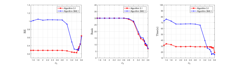
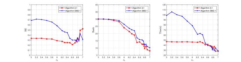
We test the two solvers on simulated data for one-bit matrix completion problems. The true matrix $M^{*}$ of rank $r^{*}$ is generated by $M^{*}\!=M_{L}^{*}(M_{R}^{*})^{\top}$ with $M_{L}^{*}\in\mathbb{R}^{n\times r^{*}}$ and $M_{R}^{*}\in\mathbb{R}^{m\times r^{*}}$ , where the entries of $M_{L}^{*}$ and $M_{R}^{*}$ are drawn i.i.d. from a uniform distribution on $[-\frac{1}{2},\frac{1}{2}]$ . We obtain one-bit observations by adding noise and recording the signs of the resulting values. Among others, the noise obeys the standard logistic distribution for case (I) and the Laplacian distribution $\textbf{Laplace}(0,b)$ for case (II) with $b=2$ . The noisy observation entries $Y_{i_{t},j_{t}}$ with $(i_{t},j_{t})\in\Omega$ are achieved by (38), where the index set $\Omega$ is given by uniform sampling. We use the relative error $\frac{\|X^{\rm out}-M^{*}\|_{F}}{\|M^{*}\|_{F}}$ to evaluate the recovery performance, where $X^{\rm out}=U^{\rm out}(V^{\rm out})^{\top}$ denotes the output of a solver.

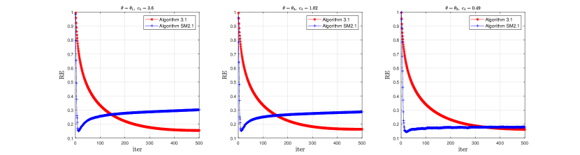
We take $n=m=2000,\,r=3r^{*}$ with $r^{*}=10$ and sample rate ${\rm SR}=0.4$ to test how the relative error (RE) and rank vary with parameter $\lambda=c_{\lambda}\max_{j\in[m]}(\|Y_{j}\|)$ . The parameter $\mu$ in model (1) is always chosen to be $\mu=10^{-8}$ . Figures 1-2 plot the average RE, rank and time (in seconds) curves by running five different instances with Algorithm 1 for $\epsilon_{1}=\epsilon_{3}=5\times 10^{-4}$ and Algorithm 2 for $\epsilon_{2}=\epsilon_{4}=10^{-3}$ , respectively. We see that when solving model (1) with smaller $\lambda$ (say, $c_{\lambda}\leq 3.2$ for Figure 1 and $c_{\lambda}\leq 6.4$ for Figure 2), Algorithm 1 returns lower RE within less time; and when solving model (1) with larger $\lambda$ (say, $c_{\lambda}>3.2$ for Figure 1 and $c_{\lambda}>6.4$ for Figure 2), the two solvers yield the comparable RE and require comparable running time. Note that model (1) with a small $\lambda$ is more difficult than the one with a large $\lambda$ . This shows that Algorithm 1 is superior to Algorithm 2 in terms of RE and running time for those difficult test instances. In addition, during the tests, we find that the relative errors yielded by the two solvers will have a rebound as the number of iterations increases, especially under the scenario where the sample ratio is low, but the RE yielded by Algorithm 2 rebounds earlier than the RE of Algorithm 1; see Figure 3 below.

Refer to caption — Figure 1: Curves of relative error, rank and time for the two solvers under Case I

6 Conclusion

For the low-rank composite factorization model (1), we proposed a majorized PAMA with subspace correction by minimizing alternately the majorization $\widehat{\Phi}_{\lambda,\mu}$ of $\Phi_{\lambda,\mu}$ at each iterate and imposing a subspace correction step on per subproblem to ensure that it has a closed-norm solution. We established the convergence of subsequences for the generated iterate sequence, and achieved the convergence of the whole iterate sequence and the column subspace sequence of factor pairs under the KL property of $\Phi_{\lambda,\mu}$ and a restrictive condition that can be satisfied by the column $\ell_{2,0}$ -norm function. To the best of our knowledge, this is the first subspace correction AM method with convergence certificate for low-rank factorization models. The obtained convergence results also provide the convergence guarantee for softImpute-ALS proposed in [13]. Numerical comparison with a line-search PALM method on one-bit matrix completions validates the efficiency of the subspace correction PAMA.

References

[1] H. Attouch, J. Bolte, P. Redont and A. Soubeyran, Proximal alternating minimization and projection methods for nonconvex problems: an approach based on the Kerdyka-Łojasiewicz inequality, Mathematics of Operations Research, 35(2010): 438-457.
[2] J. Bolte, S. Sabach, and M. Teboulle, Proximal alternating linearized minimization for nonconvex and nonsmooth problems, Mathematical Programming, 146 (2014), pp. 459–494.
[3] S. Bhojanapalli, B. Neyshabur, and N. Srebro, Global Optimality of Local Search for Low Rank Matrix Recovery, Advances in Neural Information Processing Systems, (2016), pp. 3873–3881.
[4] J. Barzilai and J. M. Borwein Two-point step size gradient methods, IMA Journal of Numerical Analysis, 8(1988), pp. 141–148.
[5] S. J. Bi, T. Ta and S. H. Pan, KL property of exponent $1/2$ of $\ell_{2,0}$ -norm and DC regularized factorizations for low-rank matrix recovery, Pacific Journal of Optimization, 18(2022): 1–26.
[6] E. J. Candès and B. Recht, Exact matrix completion via convex optimization Foundations of Computational Mathematics, 9(2009): 717–772.
[7] X. Chen and P. Tseng, Non-Interior continuation methods for solving semidefinite complementarity problems, Mathematical Programming, 95(2003): 431–474.
[8] T. Cai and W. X. Zhou, A max-norm constrained minimization approach to 1-bit matrix completion Journal of Machine Learning Research, 9(2013): 3619–3647.
[9] W. Cao, J. Sun and Z. Xu, Fast image deconvolution using closed-form thresholding formulas of $L_{q}\ (q=\frac{1}{2},\frac{2}{3})$ regularization Journal of Visual Communication and Image representation, 24(2013): 31–41.
[10] E. Chouzenoux, J. C. Pesque and A. Repetti, A block coordinate variable metric forward-backward algorithm, Journal of Global Optimization, 66(2016): 457–485.
[11] C. Ding, D. F. Sun and K. C. Toh, An introduction to a class of matrix cone programming, Mathematical Programming, 144(2014): 141–179.
[12] F. M. Dopico, A note on sin theorems for singular subspace variations, BIT Numerical Mathematics, 40(2): 395–403.
[13] T. Hastie, R. Mazumder, J. D. Lee and R. Zadeh, Matrix Completion and Low-Rank SVD via Fast Alternating Least Squares Journal of Machine Learning Research, 16(2015): 3367-3402.
[14] P. Jain, P. Netrapalli and S. Sanghavi, Low-rank matrix completion using alternating minimization In Proceedings of the 45th annual ACM Symposium on Theory of Computing (STOC), (2013): 665–674.
[15] S. Negahban and M. Wainwright, Estimation of (near) low-rank matrices with noise and high-dimensional scaling, The Annals of Statistics, 39(2011): 1069–1097.
[16] P. Ochs, Unifying abstract inexact convergence theorems and block coordinate variable metric iPiano, SIAM Journal on Optimization, 29(2019): 541–570.
[17] T. Pock and S. Sabach, Inertial proximal alternating linearized minimization (iPALM) for nonconvex and nonsmooth problems, SIAM review, 9(2016): 1756–1787.
[18] B. Recht, M. Fazel, and P. A. Parrilo, Guaranteed minimum-rank solutions of linear matrix equations via nuclear norm minimization, SIAM review, 52(2010): 471-501.
[19] R. T. Rockafellar and R. J-B. Wets, Variational analysis, Springer, 1998.
[20] F. H. Shang, Y. Y. Liu and F. J. Shang , A Unified Scalable Equivalent Formulation for Schatten Quasi-Norms, Mathematics. 8(2020):1-19.
[21] N. Srebro, J. D. M. Rennie and T. Jaakkola, Maximum-margin matrix factorization, Advances In Neural Information Processing Systems, 17, 2005.
[22] G. W. Stewart and J. G. Sun, Maximum-margin matrix factorization, Academic Press, Boston, 1990.
[23] T. Tao, S. H. Pan and S. J. Bi, Error bound of critical points and KL property of exponent $1/2$ for squared F-norm regularized factorization, Journal of Global Optimization, 81(2021): 991–1017.
[24] T. Tao, Y T. Qian and S. H. Pan, Column $\ell_{2,0}$ -norm regularized factorization model of low-rank matrix recovery and its computation, SIAM Journal on Optimization, 32(2022): 959–988.
[25] Y. Y. Xu and W. T. Yin, A globally convergent algorithm for nonconvex optimization based on block coordinate update, Journal of Scientific Computing, 72(2017): 700-734.
[26] Z. Xu, X. Chang, F. Xu and H. Zhang, $\ell_{1/2}$ regularization: A thresholding representation theory and a fast solver, IEEE Transactions on Neural Networks and Learning Systems, 23(2012): 1013–1027.

Appendix A

The following proposition states that any stationary point $(\overline{U},\overline{V})$ of problem (1) satisfies the balance, i.e., $\overline{U}^{\top}\overline{U}=\overline{V}^{\top}\overline{V}$ .

Proposition 1

Denote by $\mathcal{S}^{*}$ the set of stationary points of (1). If $\theta^{\prime}(t)\geq 0$ for $t>0$ , then $\mathcal{S}^{*}\subset{\rm crit}\,F_{\mu}$ , and hence every $(\overline{U},\overline{V})\in\mathcal{S}^{*}$ satisfies $\overline{U}^{\top}\overline{U}=\overline{V}^{\top}\overline{V}$ and $J_{\overline{U}}=J_{\overline{V}}$ , where $F_{\mu}(U,V):=f(UV^{\top})+(\mu/2)(\|U\|_{F}^{2}+\|V\|_{F}^{2})$ for $(U,V)\in\mathbb{R}^{n\times r}\times\mathbb{R}^{m\times r}$ .

Proof: Pick any $(\overline{U},\overline{V})\in\mathcal{S}^{*}$ . From Definition 2.2, it follows that for any $j\in[r]$ ,

0\in\nabla f(\overline{U}\overline{V}^{\top})\overline{V}+\mu\overline{U}+\lambda\partial\vartheta(\overline{U})\ \ {\rm and}\ \ 0\in\big{[}\nabla f(\overline{U}\overline{V}^{\top})\big{]}^{\top}\overline{U}+\mu\overline{V}+\lambda\partial\vartheta(\overline{V}).

(39)

For each $j\in J_{\overline{U}}$ , from the first inclusion in (39) and Lemma 2.2, we have

0=\nabla f(\overline{U}\overline{V}^{\mathbb{T}})\overline{V}_{\!j}+\mu\overline{U}_{j}+\lambda\theta^{\prime}(\|\overline{U}_{\!j}\|)\frac{\overline{U}_{j}}{\|\overline{U}_{\!j}\|},

and hence $\|\nabla f(\overline{U}\overline{V}^{\top})\overline{V}_{\!j}\|=\big{(}\mu+\lambda\frac{\theta^{\prime}(\|\overline{U}_{j}\|)}{\|\overline{U}_{j}\|}\big{)}\|\overline{U}_{\!j}\|$ . Recall that $\theta^{\prime}(t)\geq 0$ for $t>0$ . For each $j\in J_{\overline{U}}$ , it holds that $\|\nabla f(\overline{U}\overline{V}^{\top})\overline{V}_{\!j}\|>0$ and hence $\overline{V}_{\!j}\neq 0$ . Consequently, $J_{\overline{U}}\subset J_{\overline{V}}$ . For each $j\in J_{\overline{V}}$ , from the second inclusion in (39) and Lemma 2.2,

0\in\big{[}\nabla f(\overline{U}\overline{V}^{\top})\big{]}^{\top}\overline{U}_{j}+\mu\overline{V}_{j}+\lambda\theta^{\prime}(\|\overline{V}_{j}\|)\frac{\overline{V}_{j}}{\|\overline{V}_{j}\|},

which by using the same arguments as above implies that $\overline{U}_{\!j}\neq 0$ , and then $J_{\overline{V}}\subset J_{\overline{U}}$ . Thus, $J_{\overline{U}}=J_{\overline{V}}:=J$ . Together with equation (39), it follows that

\nabla\!f(\overline{U}\overline{V}^{\top})\overline{V}_{\!J}+\mu\overline{U}_{\!J}=0\ \ {\rm and}\ \ [\nabla\!f(\overline{U}\overline{V}^{\top})]^{\top}\overline{U}_{\!J}+\mu\overline{V}_{\!J}=0,

which implies that $\nabla\!F_{\mu}(\overline{U},\overline{V})=0$ and $(\overline{U},\overline{V})\in{\rm crit}\,F_{\mu}$ . Consequently, the desired inclusion follows. From [23, Lemma 2.2], every $(\overline{U},\overline{V})\in\mathcal{S}^{*}$ satisfies $\overline{U}^{\top}\overline{U}=\overline{V}^{\top}\overline{V}$ . $\Box$

Proposition 2

Suppose that Assumptions 1-2 holds with $\theta^{\prime}$ being strictly continuous on $\mathbb{R}_{++}$ , that there is $W^{*}\in\mathcal{W}^{*}$ with $\overline{X}^{*}$ having distinct nonzero singular values, and $\Phi_{\lambda,\mu}$ has the KL property at $(\overline{U}^{*},\overline{V}^{*})$ . Let $\delta=0.5\min\limits_{1\leq i<j\leq\overline{r}+1}[\sigma_{i}(\overline{X}^{*})\!-\!\sigma_{j}(\overline{X}^{*})]$ for $\overline{r}\!={\rm rank}(\overline{X}^{*})$ .

(i)

Then, for any $X,X^{\prime}\in\mathbb{B}(\overline{X}^{*},\delta)\cap\{X\in\mathbb{R}^{n\times m}\ |\ {\rm rank}(X)=\overline{r}\}$ and $(U,V)\in\mathbb{O}^{m,n}(X)$ and $(U^{\prime},V^{\prime})\in\mathbb{O}^{m,n}(X^{\prime})$ ,

\max\big{(}\max_{1\leq i\leq\overline{r}}\|U_{i}-U_{i}^{\prime}\|,\max_{1\leq i\leq\overline{r}}\|V_{i}-V_{i}^{\prime}\|\big{)}\leq({2}/{\delta})\|X-X^{\prime}\|_{F};

(ii)

there exists $\overline{k}\in\mathbb{N}$ such that for all $k\geq\overline{k}$ , $\overline{X}^{k}\in\mathbb{B}(\overline{X}^{*},\delta)\cap\{X\in\mathbb{R}^{n\times m}\ |\ {\rm rank}(X)=\overline{r}\}$ ,

	$\displaystyle{\rm dist}\big{(}0,\partial\Phi_{\lambda,\mu}(\overline{U}^{{k}+1},\overline{V}^{{k}+1})\big{)}$	$\displaystyle\leq c_{s}(\\|\overline{X}^{{k}+1}-\overline{X}^{{k}}\\|_{F}+\\|\widehat{X}^{{k}+1}\!\!\!-\!\overline{X}^{{k}}\\|_{F})$
		$\displaystyle+c_{s}(\\|U^{{k}+1}-\overline{U}^{{k}}\\|_{F}+\\|V^{{k}+1}\!\!\!-\!\widehat{V}^{{k}+1}\\|_{F}).$

Proof: (i) As $\overline{X}^{*}$ has distinct nonzero singular values with $\min\limits_{1\leq i<j\leq\overline{r}+1}[\sigma_{i}(\overline{X}^{*})-\sigma_{j}(\overline{X}^{*})]=2\delta$ , from Wely’s Theorem [22, Corollary 4.9], for any $X\in\mathbb{B}(\overline{X}^{*},\delta)\cap\{X\in\mathbb{R}^{n\times m}\,|\,{\rm rank}(X)=\overline{r}\}$ , $\min\limits_{1\leq i<j\leq\overline{r}+1}[\sigma_{i}(X)-\sigma_{j}(X)]\geq\delta$ . Fix any $X,X^{\prime}\in\mathbb{B}(\overline{X}^{*},\delta)\cap\{X\in\mathbb{R}^{n\times m}\,|\,{\rm rank}(X)=\overline{r}\}$ and any $(U,V)\in\mathbb{O}^{m,n}(X)$ and $(U^{\prime},V^{\prime})\in\mathbb{O}^{m,n}(X^{\prime})$ . By [12, Theorem 2.1], we get the result.

(ii) As $\overline{X}^{*}$ is a cluster point of $\{\widehat{X}^{k}\}$ and $\{\overline{X}^{k}\}$ by Theorem 4.2 and $\lim_{k\to\infty}\|\overline{X}^{k}\!-\!\widehat{X}^{k}\|_{F}=0$ by Corollary 4.1 (iv), there exists $\overline{k}\in\mathbb{N}$ such that $\overline{X}^{\overline{k}+1},\widehat{X}^{\overline{k}+1}\in\mathbb{B}(\overline{X}^{*},\delta/2)\cap\{X\in\mathbb{R}^{n\times m}\,|\,{\rm rank}(X)=\overline{r}\}$ . From part (i) with $X=\overline{X}^{\overline{k}+1}$ and $X^{\prime}=\widehat{X}^{\overline{k}+1}$ , (25)-(26) hold with $R_{1}^{\overline{k}+1}=R_{2}^{\overline{k}}=I_{\overline{r}}$ , so Lemma 4.2 holds with $A_{1}^{\overline{k}+1}=B_{1}^{\overline{k}}=I_{\overline{r}}$ . By the local Lipschitz continuity of $\nabla\vartheta_{\!J}$ with $J=[\overline{r}]$ , inequalities (29a)-(29b) hold with $k=\overline{k}$ . From Proposition 4.1,

	$\displaystyle{\rm dist}\big{(}0,\partial\Phi_{\lambda,\mu}(\overline{U}^{\overline{k}+1},\overline{V}^{\overline{k}+1})\big{)}$	$\displaystyle\leq c_{s}(\\|\overline{X}^{\overline{k}+1}-\overline{X}^{\overline{k}}\\|_{F}+\\|\widehat{X}^{\overline{k}+1}-\overline{X}^{\overline{k}}\\|_{F})$
		$\displaystyle\quad+c_{s}(\\|U^{\overline{k}+1}-\overline{U}^{\overline{k}}\\|_{F}+\\|V^{\overline{k}+1}-\widehat{V}^{\overline{k}+1}\\|_{F}).$		(40)

Since $\Phi_{\lambda,\mu}$ has the KL property at $(\overline{U}^{*},\overline{V}^{*})$ , there exist $\eta>0$ , a neighborhood $\mathcal{N}$ of $(\overline{U}^{*},\overline{V}^{*})$ , and a continuous concave function $\varphi\!:[0,\eta)\to\mathbb{R}_{+}$ satisfying Definition 2.3 (i)-(ii) such that for all $(U,V)\in\mathcal{N}\cap[\Phi_{\lambda,\mu}(\overline{U}^{*},\overline{V}^{*})<\Phi_{\lambda,\mu}<\Phi_{\lambda,\mu}(\overline{U}^{*},\overline{V}^{*})+\eta]$ ,

\varphi^{\prime}(\Phi_{\lambda,\mu}(U,V)-\Phi_{\lambda,\mu}(\overline{U},\overline{V})){\rm dist}(0,\partial\Phi_{\lambda,\mu}(U,V))\geq 1.

(41)

Let $\Gamma_{k,k+1}:=\!\varphi\big{(}\Phi_{\lambda,\mu}(\overline{U}^{k},\overline{V}^{k})-\Phi_{\lambda,\mu}(\overline{U}^{*},\overline{V}^{*})\big{)}\!-\!\varphi\big{(}\Phi_{\lambda,\mu}(\overline{U}^{k+1},\overline{V}^{k+1})\!-\!\Phi_{\lambda,\mu}(\overline{U}^{*},\overline{V}^{*})\big{)}$ . If necessary by increasing $\overline{k}$ , $(\overline{U}^{\overline{k}+1},\overline{V}^{\overline{k}+1})\!\in\!\mathcal{N}\cap[\Phi_{\lambda,\mu}(\overline{U}^{*},\overline{V}^{*})<\Phi_{\lambda,\mu}<\Phi_{\lambda,\mu}(\overline{U}^{*},\overline{V}^{*})+\eta]$ . Then

\varphi^{\prime}(\Phi_{\lambda,\mu}(\overline{U}^{\overline{k}+1},\overline{V}^{\overline{k}+1})-\Phi_{\lambda,\mu}(\overline{U}^{*},\overline{V}^{*})){\rm dist}(0,\partial\Phi_{\lambda,\mu}(\overline{U}^{\overline{k}+1},\overline{V}^{\overline{k}+1}))\geq 1.

Together with the concavity of $\varphi$ , it is easy to obtain that

\Phi_{\lambda,\mu}(\overline{U}^{\overline{k}+1},\overline{V}^{\overline{k}+1})-\Phi_{\lambda,\mu}(\overline{U}^{\overline{k}+2},\overline{V}^{\overline{k}+2})\leq{\rm dist}(0,\partial\Phi_{\lambda,\mu}(\overline{U}^{\overline{k}+1},\overline{V}^{\overline{k}+1}))\Gamma_{\overline{k}+1,\overline{k}+2}.

Combining this inequality with Corollary 4.1 (iii) and the above (A majorized PAM method with subspace correction for low-rank composite factorization model), it holds that

\sqrt{a}\Xi^{\overline{k}+2}\leq\frac{\sqrt{a}}{2}\Xi^{\overline{k}+1}+\frac{\sqrt{a}c_{s}}{2}\Gamma_{\overline{k}+1,\overline{k}+2}\quad{\rm with}\ a=\min(\frac{\overline{\gamma}}{4},\frac{\overline{\gamma}}{16\overline{\beta}^{2}}),

where $\Xi^{k+1}:=\|\overline{X}^{\overline{k}+1}\!-\!\overline{X}^{\overline{k}}\|_{F}+\|\widehat{X}^{\overline{k}+1}\!-\!\overline{X}^{\overline{k}}\|_{F}+\|U^{\overline{k}+1}\!-\overline{U}^{\overline{k}}\|_{F}+\|V^{\overline{k}+1}-\widehat{V}^{\overline{k}+1}\|_{F}$ . By Theorem 4.2 (iii), $\Xi^{\overline{k}+1}+c_{s}\varphi\big{(}\Phi_{\lambda,\mu}(\overline{U}^{\overline{k}+1},\overline{V}^{\overline{k}+1})-\Phi_{\lambda,\mu}(\overline{U}^{*},\overline{V}^{*})\big{)}\leq\delta$ and $\|\overline{X}^{k+1}\!-\!\widehat{X}^{k+1}\|_{F}\leq 0.25\delta$ for all $k\geq\overline{k}$ (if necessary by increasing $\overline{k}$ ). Thus, we have $\Xi^{\overline{k}+2}\leq 0.5\delta$ and hence $\overline{X}^{\overline{k}+2},\widehat{X}^{\overline{k}+2}\in\mathbb{B}(\overline{X}^{*},\delta)\cap\{X\in\mathbb{R}^{n\times m}\,|\,{\rm rank}(X)=\overline{r}\}$ . By repeating the above arguments, we have

\sqrt{a}\Xi^{\overline{k}+3}\leq\frac{\sqrt{a}}{2}\Xi^{\overline{k}+2}+\frac{\sqrt{a}c_{s}}{2}\Gamma_{\overline{k}+2,\overline{k}+3},

This implies that $\sqrt{a}(\Xi^{\overline{k}+2}+\Xi^{\overline{k}+3})\leq\frac{\sqrt{a}}{2}\Xi^{\overline{k}+1}+\frac{\sqrt{a}c_{s}}{a}\Gamma_{\overline{k}+1,\overline{k}+3}$ , so $\overline{X}^{\overline{k}+3},\widehat{X}^{\overline{k}+3}\in\mathbb{B}(\overline{X}^{*},\delta)\cap\{X\in\mathbb{R}^{n\times m}\,|\,{\rm rank}(X)=\overline{r}\}$ . By induction, we can obtain the desired result. $\Box$

Appendix B: A line-search PALM method for problem (1).

As mentioned in the introduction, the iterations of the PALM methods in [2, 17, 25] depend on the Lipschitz constants of $\nabla_{U}F(\cdot,V^{k})$ and $\nabla_{V}F(U^{k+1},\cdot)$ . An immediate upper estimation for them is $L_{f}\max\{\|V^{k}\|^{2},\|U^{k+1}\|^{2}\}$ , but it is too large and will make the performance of PALM methods worse. Here we present a PALM method by searching a favourable estimation for them. For any given $(U,V)$ and $\tau>0$ , let $\mathcal{Q}_{U}(U^{\prime},V^{\prime};U,V,\tau)$ and $\mathcal{Q}_{V}(U^{\prime},V^{\prime};U,V,\tau)$ be defined by

	$\displaystyle\mathcal{Q}_{U}(U^{\prime},V^{\prime};U,V,\tau):=F(U,V)+\langle\nabla_{U}F(U,V),U^{\prime}-U\rangle+({\tau}/{2})\\|U^{\prime}-U\\|_{F}^{2},$
	$\displaystyle\mathcal{Q}_{V}(U^{\prime},V^{\prime};U,V,\tau):=F(U,V)+\langle\nabla_{V}F(U,V),V^{\prime}-V\rangle+({\tau}/{2})\\|V^{\prime}-V\\|_{F}^{2}.$

The iterations of the line-search PALM method are described as follows.

Algorithm 2 (A line-search PALM method)

Initialization: Choose $\varrho_{1}>1,\varrho_{2}>1,0<\underline{\alpha}<\overline{\alpha}$ and an initial point $(U^{0},V^{0})\in\mathbb{X}_{r}$ .
For $k=0,1,2,\ldots$

1.

Select $\alpha_{k}\in[\underline{\alpha},\overline{\alpha}]$ and compute

$U^{k+1}\in\mathop{\arg\min}_{U\in\mathbb{R}^{n\times r}}\mathcal{Q}_{U}(U,V^{k};U^{k},V^{k},\alpha_{k}).$
2.
while $F(U^{k+1},U^{k})>\mathcal{Q}_{U}(U^{k+1},V^{k};U^{k},V^{k},\alpha_{k})$ do
- (a)
  
  $\tau_{k}=\varrho\tau_{k}$ ;
- (b)
  
  Compute $U^{k+1}\in\mathop{\arg\min}_{U\in\mathbb{R}^{n\times r}}\mathcal{Q}_{U}(U,V^{k};U^{k},V^{k},\tau_{k})$
end (while)
3.

Select $\alpha_{k}\in[\underline{\alpha},\overline{\alpha}]$ . Compute

$V^{k+1}\in\!\mathop{\arg\min}_{V\in\mathbb{R}^{m\times r}}\mathcal{Q}_{V}(U^{k+1},V;U^{k+1},V^{k},\alpha_{k}).$
4.
while $F(U^{k+1},V^{k+1})>\mathcal{Q}_{V}(U^{k+1},V^{k+1};U^{k+1},V^{k},\tau_{k})$ do
- (a)
  
  $\alpha_{k}=\varrho_{2}\alpha_{k}$ ;
- (b)
  
  Compute $V^{k+1}\in\mathop{\arg\min}_{V\in\mathbb{R}^{m\times r}}\mathcal{Q}_{V}(U^{k+1},V;U^{k+1},V^{k},\alpha_{k})$ .
end (while)
5.

Let $k\leftarrow k+1$ , and go to step 1.

end

Remark 1

In the implementation of Algorithm 2, we use the Barzilai-Borwein (BB) rule [4] to capture the initial $\alpha_{k}$ in steps 1 and 3. That is, $\alpha_{k}$ in step 1 is given by

\max\Big{\{}\min\Big{\{}\frac{\|\langle\nabla_{U}F(U^{k},V^{k})-\nabla_{U}F(U^{k-1},V^{k})\|_{F}}{\|U^{k}-U^{k-1}\|_{F}}\Big{)},\underline{\alpha}\Big{\}},\overline{\alpha}\Big{\}},

while $\alpha_{k}$ in step 2 is chosen to be

\max\Big{\{}\min\Big{\{}\frac{\|\langle\nabla_{V}F(U^{k},V^{k})-\nabla_{V}F(U^{k},V^{k-1})\|_{F}}{\|V^{k}-V^{k-1}\|_{F}}\Big{)},\underline{\alpha}\Big{\}},\overline{\alpha}\Big{\}}.

$\displaystyle\big{\\|}\overline{U}^{k+1}\!-\!\widehat{U}^{k+1}A^{k+1}\big{\\|}_{F}$	$\displaystyle=\big{\\|}\widetilde{R}_{\!J}^{k+1}\overline{D}_{1}^{k+1}\!-\!\widehat{P}_{\!J}^{k+1}R_{1}^{k+1}\widehat{D}_{1}^{k+1}\big{\\|}_{F}$
	$\displaystyle\leq\\|\overline{D}_{1}^{k+1}-\widehat{D}_{1}^{k+1}\\|_{F}+\\|\widehat{D}_{1}^{k+1}\\|\\|\widetilde{R}_{J}^{k+1}-\widehat{P}^{k+1}_{{J}}R_{1}^{k+1}\\|_{F}$
	$\displaystyle\leq\frac{\sqrt{\alpha}+4\overline{\beta}}{2\alpha}\\|\overline{X}^{k+1}-\widehat{X}^{k+1}\\|_{F}$	(27)

$\displaystyle\\|\overline{V}^{k+1}\!-\!\widehat{V}^{k+1}A^{k+1}\\|_{F}$	$\displaystyle=\big{\\|}\overline{P}_{\!J}^{k+1}\overline{D}_{\!J}^{k+1}-\widetilde{Q}_{\!J}^{k+1}R_{1}^{k+1}\widehat{D}_{1}^{k+1}\big{\\|}_{F}$
	$\displaystyle\leq\\|\overline{D}_{1}^{k+1}-\widehat{D}_{1}^{k+1}\\|_{F}+\\|\widehat{D}_{1}^{k+1}\\|\\|\overline{P}_{\!J}^{k+1}-\widetilde{Q}_{\!J}^{k+1}R_{1}^{k+1}\\|_{F}$
	$\displaystyle\leq\frac{\sqrt{\alpha}+4\overline{\beta}}{2\alpha}\\|\overline{X}^{k+1}-\widehat{X}^{k+1}\\|_{F}\quad{\rm for\ each}\ k\geq\widetilde{k}.$	(28)

$\displaystyle\\|S^{k+1}\!\\|_{F}$	$\displaystyle\leq\\|\nabla\!f(\overline{X}^{k+1}\!)\overline{V}^{k+1}\!-\!\nabla\!f(\overline{X}^{k})\overline{V}^{k}B^{k}\\|_{F}\!+\!L_{\!f}\overline{\beta}\\|\widehat{X}^{k+1}\!\!-\!\overline{X}^{k}\!\\|_{F}+\!\mu\\|\overline{U}^{k+1}\!-\!U^{k+1}B^{k}\\|_{F}$
	$\displaystyle\quad\ +\!\gamma_{1,k}(\overline{\beta}/{\sqrt{\alpha}})\\|U^{k+1}\!-\!\overline{U}^{k}\\|_{F}+\lambda\\|\nabla\vartheta_{\!J}(U_{\!J}^{k+1})B_{1}^{k}-\nabla\vartheta_{\!J}(\overline{U}_{\!J}^{k+1})\\|_{F},$	(33)
$\displaystyle\\|T^{k+1}\\|_{F}$	$\displaystyle\leq\\|\nabla\!f(\overline{X}^{k+1})\overline{U}^{k+1}\!-\!\nabla\!f(\widehat{X}^{k+1})\widehat{V}^{k+1}A^{k+1}\\|_{F}+L_{\!f}\overline{\beta}\\|\widehat{X}^{k+1}\!-\!\overline{X}^{k+1}\\|_{F}$
	$\displaystyle\quad\ +\mu\\|\overline{V}^{k+1}\!-V^{k+1}A^{k+1}\\|_{F}+\gamma_{2,k}(\overline{\beta}/{\sqrt{\alpha}})\\|V^{k+1}\!-\widehat{V}^{k+1}\\|_{F}$
	$\displaystyle\quad\ +\lambda\\|\nabla\vartheta_{\!J}(V_{\!J}^{k+1})A_{1}^{k+1}-\nabla\vartheta_{\!J}(\overline{V}_{\!J}^{k+1})\\|_{F}$	(34)

	$\displaystyle\\|S^{k+1}\\|_{F}$	$\displaystyle\leq\big{[}L_{f}\overline{\beta}+0.5\alpha^{-1}(c_{f}+\mu+\!\lambda)(\sqrt{\alpha}\!+\!4\overline{\beta})\big{]}\\|\overline{X}^{k+1}-\overline{X}^{k}\\|_{F}$
		$\displaystyle\quad+(\mu\!+\!\lambda+\gamma_{1,k})({\overline{\beta}}/{\sqrt{\alpha}})\\|U^{k+1}-\overline{U}^{k}\\|_{F}+L_{\!f}\overline{\beta}\\|\widehat{X}^{k+1}\!\!-\!\overline{X}^{k}\!\\|_{F}.$		(35)