A mathematical Model for Rogue Waves,
using Saint-Venant Equations with Friction

We denote by $q=q(x,t)$ the ocean depth at a point $x$ at a time $t$, and $m=m(x,t)$ the corresponding flux. We have $m=q\ u$, where $u$ is the water velocity. The relative velocity of the waves of the ocean surface is given by

$$c\ =\ \sqrt{gq}\ \ \ \ (=c(q))\ .$$

We denote by $k>0$ the friction coefficient of Strickler and we consider as a simplification purpose that the bottom is flat. In this configuration, the Saint-Venant model reads

(1.1)

$$q_{t}\ +\ m_{x}\ =\ 0\ ,$$

(1.2)

$$m_{t}\ +\ 2u\ m_{x}\ +\ \left({c^{2}-u^{2}}\right)\ q_{x}\ +\ k\ \left|{u}\right|u\ =\ 0\ \ .$$

We shall use the representation of waves proposed in  [3] when a source term (here $k\left|{u}\right|u$)
is present. The different states of the same wave are described by a segment of a straight line

(1.3)

$$m\ =\ A\ q\ -\ B\ ,$$

in the phase plane, that is the plane $(q,m)$ here. The parameter $A$ is a constant which corresponds to the wave velocity, of the form $A=u_{ref}-c(q_{ref})$ or $A=u_{ref}+c(q_{ref})$ depending if the wave is travelling eastwards (sign $+$) or westwards (sign $-$) and for a given reference state $M_{ref}=(q_{ref},m_{ref}),$ with $m_{ref}=q_{ref}u_{ref},$ of course. The parameter $B$ is also a constant and is determined by the reference state since $B=m_{ref}+A\ q_{ref}.$ We denote by $M_{0}$ the state of the ocean far on the west side, and by $M_{*}$ the state of the ocean far on the east side. In both cases, the distances are supposed to be larger than the reference wavelength $\lambda$ proposed in (0.1), which allows to use the Saint-Venant model. We suppose that these states also corresponds to reference velocity equal to zero; this assumption is linked to the hypothesis of a flat bottom of the ocean. That way $M_{0}$ represents a state $M_{0}=\left({q_{0},0}\right)$ and $M_{*}$ represents a state $M_{*}=\left({q_{*},0}\right)$. We suppose

$$q_{0}\ >\ q_{*}\ \ .$$

A difference $q_{0}-q_{*}$ of a few decimeters is enough even for a wide depth of the ocean. The profile of the initial state is made of two branches which meet in a state $P=\left({q_{P},m_{P}}\right)$ for example at $x=0,$ which corresponds to the choice of the origin. From the state $P$ to the state $M_{*}$, that is on the East side, the profile is decreasing and referred to the state $M_{*}$. The corresponding states are so situated on the straight line

$$m\ =\ c_{*}\ \left({q-q_{*}}\right)\ \ ,\$$

with $c_{*}=c(q_{*})=\sqrt{gq_{*}}\ .$ As a matter of fact, we have $A=c_{*}$ and $B=c_{*}q_{*}$ for this part of the wave profile. The explicit formulation of the profile is obtained, following  [1], by inverting the profile relation

(1.4)

$$\psi_{E}(q)\ =\ x\ ,$$

where the index $E$ stands for East. The inverse profile $\psi_{E}(q)$ is determined by integrating

$$\psi_{E}^{\prime}(q)\ =\ \frac{B^{2}-c^{2}q^{2}}{k\left|{Aq-B}\right|\left({Aq-B}\right)}\ \ ,\ \ \psi_{E}(q_{P})=0\ \ .$$

We need to have $q_{*}\ <\ q_{0}\ <\ q_{P}$ , in order to ensure an increasing profile on the West side, then a decreasing one on the East side. We get that way a positive flux: $Aq-B=c_{*}\left({q-q_{*}}\right)\ >\ 0$, and by writing $\xi=\frac{q}{q_{*}}$ we get

$$\psi_{E}^{\prime}(q)\ =\ \frac{1-\xi^{3}}{k\left({1-\xi}\right)^{2}}\ =\ \frac{1+\xi+\xi^{2}}{k\left({1-\xi}\right)}\ =\ \frac{1}{k}\ \left({\ \frac{3}{1-\xi}\ -2\ -\xi}\right)\ ,$$

thus

$$\psi_{E}(q)\ =\ -\frac{3q_{*}}{k}\ ln\left({\frac{q-q_{*}}{q_{P}-q_{*}}}\right)\ +\ \frac{2}{k}\ \left({q_{P}-q}\right)\ +\ \frac{1}{2kq_{*}}\ \left({q_{P}^{2}-q_{*}^{2}}\right)\ .$$

By inverting this function $\psi_{E}(q)$ and using  (1.4) we get $q$ as a decreasing function of $x$ which is equal to $q_{P}$ when $x=0\ .$ For the West side of the profile, with the index $W$, the reference state $M_{ref}=\left({q_{ref},m_{ref}}\right)\$must correspond to a depth satisfying

$$q_{ref}\ \geq\ q_{P}\ (\geq q_{0})\ \ ,$$

in order to ensure an increasing profile. The reference velocity associated with the state $M_{ref}$ that is

$$A_{ref}\ =\ \frac{m_{ref}}{q_{ref}}\ +\ c_{ref}\ \ \ ,\ \ \ with\ \ c_{ref}\ =\ c(q_{ref})\ =\ \sqrt{gq_{ref}}\ \ ,$$

is also the velocity of the West side profile of the wave and is positive. The straight line representing this West profile in the phase plane has the form

$$m\ =\ m_{ref}\ +\ A_{ref}\ \left({q-q_{ref}}\right)\ ,$$

and passes by the state $M_{0}\ =(q_{0},0)$. Hence

$$m_{ref}\ =\ A_{ref}\ \left({q_{ref}-q_{0}}\right)\ \ \ ,\ \ B_{ref}\ =\ c_{ref}\ q_{ref}\ \ .$$

The invert profile is described by a function $\psi_{W}$ satisfying

$$\psi_{W}^{\prime}(q)\ =\ \frac{B_{ref}^{2}-c_{ref}^{2}q_{ref}^{2}}{k\ \left({A_{ref}q-B_{ref}}\right)^{2}}\ \ ,\ \ \psi_{W}(q_{P})\ =\ 0\ \ ,$$

with $q_{0}\ \leq\ q_{P}\ \leq\ q_{ref}\ .$ The initial West side profile of the wave is then obtained by inverting, for any $x<0$,

(1.5)

$$\psi_{W}(q)\ =\ x\ .$$

We set

$$\xi\ =\ \frac{q}{q_{ref}}\ \ \ ,\ \ \ \xi_{0}\ =\ \frac{q_{0}}{q_{ref}}\ \ \ ,\ \ F_{ref}\ =\ \frac{m_{ref}}{c_{ref}\ q_{ref}}\ ,\ (\ Froude\ number\ )\ ,\$$

to obtain

$$\psi_{W}(q)\ =\ \frac{q_{ref}}{k\ \left({F_{ref}+1}\right)^{2}}\ \int_{\frac{q_{P}}{q_{ref}}}^{\frac{q}{q_{ref}}}{\left({-\xi-2\xi_{0}+\frac{\xi_{0}\left({\xi_{0}-4}\right)}{\xi-\xi_{0}}+\frac{1-\xi_{0}^{3}}{\left({\xi-\xi_{0}}\right)^{2}}}\right)\ d\xi}\ \ ,$$

that is

$$\psi_{W}(q)=K\left[{\frac{q_{P}^{2}-q^{2}}{2\ q_{ref}}+2\frac{q_{0}}{q_{ref}}\left({q_{P}-q}\right)+\frac{q_{0}}{q_{ref}}\left({q_{0}-4q_{ref}}\right)ln\left({\frac{q-q_{0}}{q_{P}-q_{0}}}\right)+\frac{\left({q_{ref}^{3}-q_{0}^{3}}\right)\left({q-q_{P}}\right)}{q_{ref}\left({q-q_{0}}\right)\left({q_{P}-q_{0}}\right)}}\right]$$

with

$$K\ =\ \frac{1}{k\ \left({F_{ref}+1}\right)^{2}}\ \ .$$

The whole initial profile is now given by  (1.5) for $x<0$ and by  (1.4) for $x>0$. It corresponds to an increasing function $q(x,0)$ for $x<0$ and a decreasing one for $x>0$, which is continuous at $x=0$ where its value is $q=q_{P}$.

The wave profile is expected to propagate eastwards, with the respective velocities $A_{ref}$ and $c_{*}$ which are different for each part West or East. Since the west profile moves lightly faster, the crest of the profile will move up, at the junction of the two parts. The left side of this crest corresponds to the continuity of the West profile, extropolated for depth values $q$ going from $q_{P}$ to the maximal value $q_{ref}$.

The right part of the crest corresponds to a discontinuity, that is a shock wave, whose location is imposed by the mass conservation. At any time $t$ the water contained in the bump under the crest comes from the column of water of length $\left({A_{ref}-c_{*}}\right)t\$shifted since the initial time. We denote by $q_{l}(t)$ and $q_{r}(t)$ the water depths on the left side (index $l$) and on the right side (index $r$) of the discontinuity, and by $x_{0}(t)$ its position. We always have

$$q_{*}\ \leq\ q_{r}(t)\ \leq\ q_{P}\ \leq\ q_{l}(t)\ \leq\ q_{ref}\ .$$

As the West profile is moving with the constant velocity $A_{ref}$, we get it by simply inverting for any time $t$, the relation

$$\psi_{W}(q)\ =\ x\ -\ A_{ref}t\ \$$

for $x<x_{0}(t)$, with the function $\psi_{W}$ defined above. By the same way, the East profile is obtained by inverting the relation

$$\psi_{E}(q)\ =\ x\ -\ c_{*}t\$$

for $x>x_{0}(t)$, with the function $\psi_{E}$ defined above. For a given time $t$, the depths $q_{l}t)$ and $q_{r}(t)$, and the shock position $x_{0}(t)$ are linked by three conditions, entailing three equations. The first equation says that $q_{l}(t)$ is the value of the West profile at $x=x_{0}(t)$, that is

$$\psi_{W}(q_{l}(t))\ =\ x_{0}(t)\ -\ A_{ref\ }t\ .$$

The second equation says that $q_{r}(t)$ is the value of the East profile at $x=x_{0}(t)$, that is

$$\psi_{E}(q_{r}(t))\ =\ x_{0}(t)\ -\ c_{*}\ t\ .$$

The third equation is given by the compatibility relation of Rankine-Hugoniot

(2.1)

$$\displaystyle\left({\displaystyle q_{l}(t)-q_{r}(t)}\right)\displaystyle\sqrt{\displaystyle g\frac{\displaystyle q_{r}(t)+q_{l}(t)}{\displaystyle 2q_{r}(t)q_{l}(t)}}\ +\ \frac{\displaystyle A_{\displaystyle ref}\ q_{0}}{\displaystyle q_{l}(t)}\ -\ \frac{\displaystyle c_{*}\ q_{*}}{\displaystyle q_{r}(t)}\ =\ A_{\displaystyle ref}\ -\ c_{*}\ ,$$

which ensures the mass conservation. A dichotomy method running on the parameter $x_{0}(t)$ allows the simultaneous determination of these three parameters. For practical purposes it is however easier to determine $x_{0}(t)$ by checking directly the mass conservation. Let us consider two points $x_{1}$ and $x_{2}$ such that

$$x_{1}\ +\ A_{ref}\ t\ <\ x_{0}(t)\ <\ x_{2}\ +\ c_{*}\ t\ .\$$

If it is not the case in a first choice, one can increase $x_{2}$ or decrease $x_{1}$ sufficiently. We denote by $M_{0}$ the mass of water laying between the two points $x_{1}$ and $x_{2}$ at the initial time:

$$M_{0}\ =\ \int_{x_{1}}^{x_{2}}{q(x,0)\ dx}\ =\ \int_{x_{1}}^{0}{q_{W}(x,0)\ dx}\ +\ \int_{0}^{x_{2}}{q_{E}(x,0)\ dx}\ ,$$

where $q_{W}$ and $q_{E}$ are the respectives depths of the West and East profiles. The same mass $M_{0}$ has to be found at any time $t$ between the two trajectories of equations

(2.2)

$$x_{1}^{\prime}(t)\ =\ A_{\displaystyle ref}\ -\ \frac{\displaystyle q_{\displaystyle ref}c_{\displaystyle ref}}{\displaystyle q_{W}\displaystyle\left({\displaystyle x_{1}(t)-A_{\displaystyle ref}t}\right)}\ \ ,\ x_{1}(0)\ =\ x_{1}\ ,$$

and

(2.3)

$$x_{2}^{\prime}(t)\ =\ c_{*}\ \displaystyle\left({\displaystyle 1-\frac{\displaystyle q_{*}}{\displaystyle q_{E}\displaystyle\left({\displaystyle x_{2}(t)-c_{*}t}\right)}}\right)\ \ ,\ \ x_{2}(0)\ =\ x_{2}\ ,$$

which means that the relation $M(t)\ =\ M_{0}$ always occurs, with

$$M(t)\ =\ \int_{x_{1}(t)}^{x_{2}(t)}{q(x,t)\ dx}\ .$$

We remark that the mass $M(t)$ may be explicitely calculated from the relation

$$M(t)=\int_{q_{1}(t)}^{q_{l}(t)}{q\ \psi_{W}^{\prime}(q)\ dq}\ +\ \int_{q_{r}(t)}^{q_{2}(t)}{q\ \psi_{E}^{\prime}(q)\ dq}\ ,$$

where $q_{1}(t)=q_{W}(x_{1}(t))\ ,\ q_{2}(t)=q_{E}(x_{2}(t))\ .$ This calculation involves only primitives of rationnal fractions. More simply, using the computing files giving $q_{W}$ on the West side of a point $x_{0}$ and $q_{E}$ on the East side of this point $x_{0}$, one can compute

$$F(x_{0})\ =\ \int_{x_{1}(t)}^{x_{0}}{q_{W}\ dx\ }+\ \int_{x_{0}}^{x_{2}(t)}{q_{E}\ dx}\ ,$$

and next determine $x_{0}=x_{0}(t)$ such that

$$F(x_{0})\ =\ M_{0}$$

by noticing that $F$ is an increasing function.

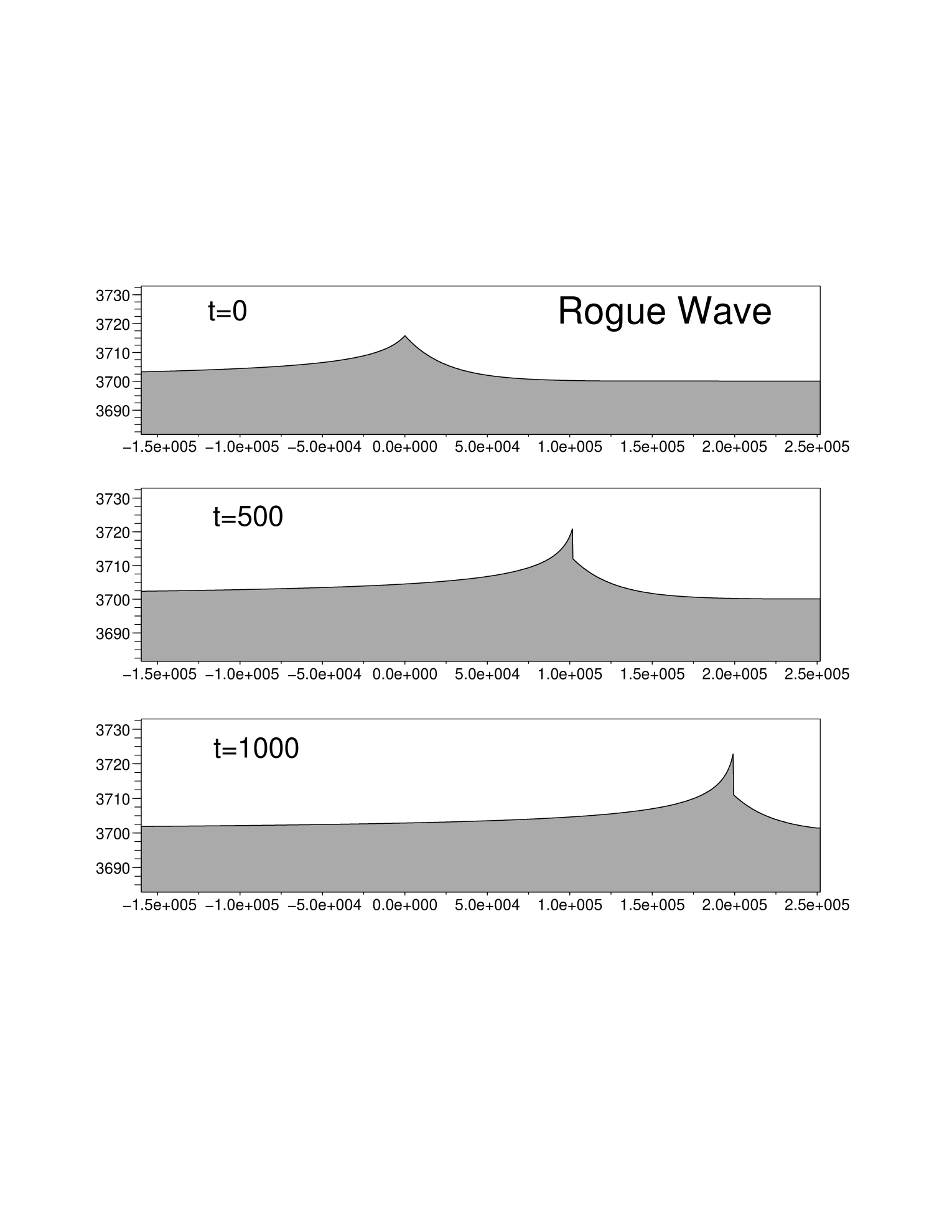
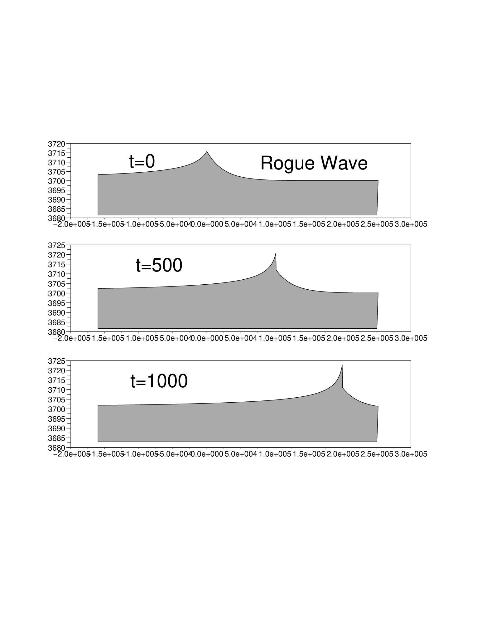
This last process has been used to compute the results shown on the figure above. For this example, we have taken $q_{*}=3700\ m$ and $q_{0}=3700.2\ m$, then $q_{ref}$ at its maximal value, that is $q_{ref}=3731.6737\ m$ here. This choice leads to the value of $q_{P}$, which is $q_{P}=3715.8087\ m$ here. The friction coefficient was taken equal to $k=0.45\ .$ We have to notice that the value of the friction coefficient is strongly linked to the wavelength of the profiles since the smallest frictions give the larger wavelengths. For terrestrial hydraulic flows (rivers or estuaries for example) the values of the friction coefficient is far smaller, of the order of $10^{-3}$ but corresponds to far less deep flows. It seems natural to consider that for larger depths this parameter has to be upgraded. At the time $t=1000$, the shock amplitude $q_{l}-q_{r}$ reaches the value $11\ m$, between the two cells adjascent to the computed position of $x_{0}(t)$ . The relative error on the mass is of order of $10^{-4}$ (mainly due to the meshsize), and the trajectories  (2.2) and  (2.3) were approached by a simple trapezoid formula, since the depth has a small variation along the trajectories $x_{1}(t)$ and $x_{2}(t)$ when they are chosen relatively far from the shock.

By upgrading lightly the value of $q_{0}$, one get more important shock amplitudes. For the next example, with $q_{0}=3700.8\ m$, we obtain the values $q_{ref}=3763.8773,$ and $q_{P}=3731.8248$. The computed shock amplitude $q_{l}-q_{r}$ is equal to $33.787\ m$. The wave crest culminates at more than 50 meters above the sea level.

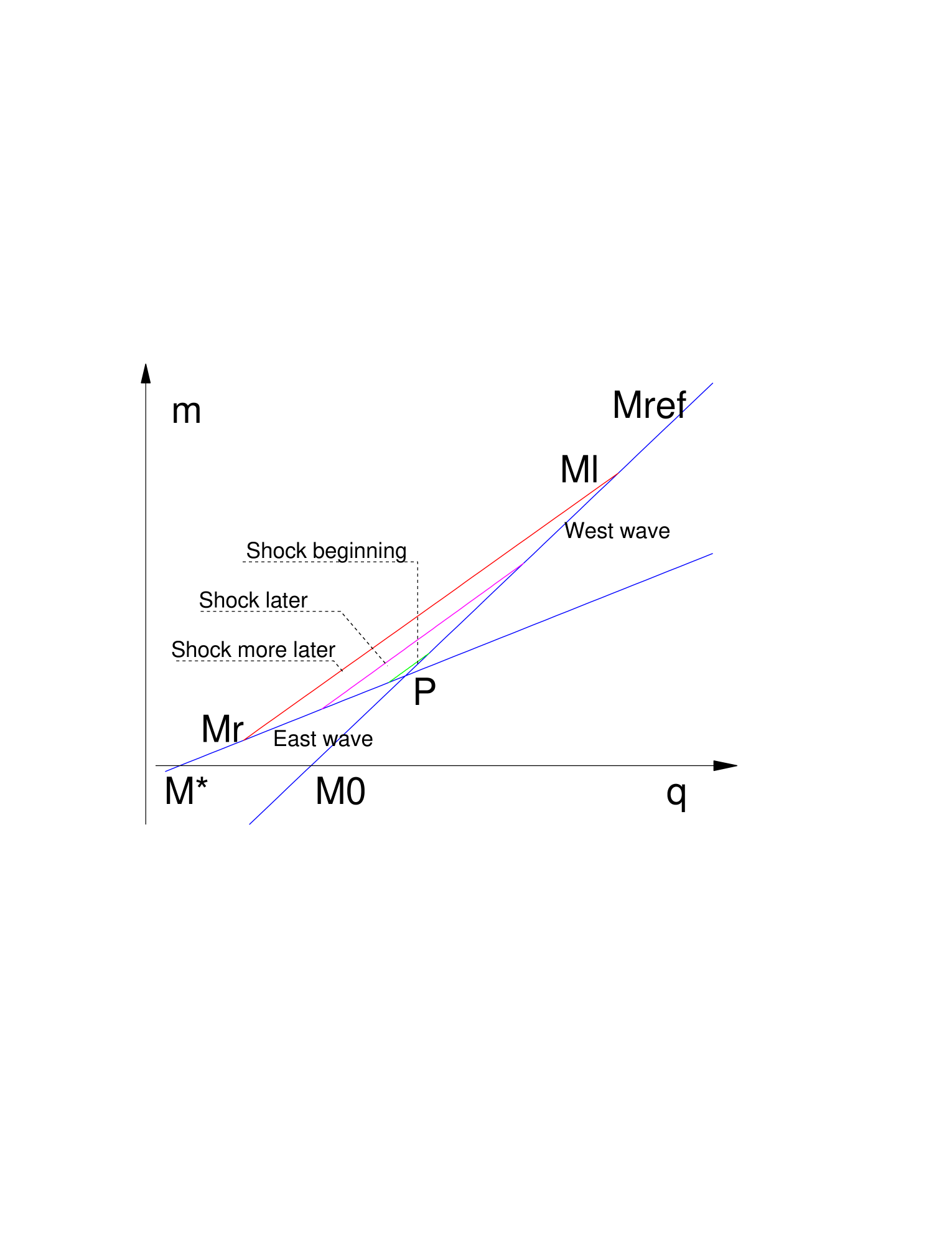
We propose a graphic interpretation in the phase plane $(q,m)$ using the picture below.

The states $M_{*}$ and $M_{0}$ are represented on the $q-$axis. The line passing through $M_{*}$ corresponds to the East wave, of equation $m=c_{*}(q-q_{*})$. The line passing through $M_{0}$ corresponds to the West wave, of equation $m=A_{ref}(q-q_{0})$. These two lines meet at the point $P$. The shock wave is represented by the segment $M_{l}M_{r}$, with $M_{l}$ sliding along the West wave line, from $P$ to $M_{ref}$ and $M_{r}$ sliding along the East wave line, from $P$ to $M_{*}$. This segment $M_{l}M_{r}$ is not exactly a straight one, and its equation is obtained from the Rankine Hugoniot condition  (2.1). The maximal amplitude is reached when the first event between $M_{l}$ reaching $M_{ref}$ or $M_{r}$ reaching $M_{*}$ occurs. After that time the wave is expected to collapse. The scaling of the picture has been strongly modified for readability, since in the real example all those lines are so close to one another that it is impossible to perceive any difference.

This study shows that the outbreak of these waves is due to a differential in the pressure field, resulting from two waves with different profiles, with close but different velocities and sufficiently large wavelengths. The water is pushed up from this pressure effect together with a friction effect. The later behaviour is not studied here: one expects that, when $q_{l}(t)$ reaches the la value $q_{ref}$ (which occurs in a finite time), a backwards wave will appear, with a negative velocity, and will provoke strong perturbations on the West profile near the wave crest, which will collapse soon. However this backwards wave will have a shorter wavelength, probably too small to fit up with the use of the Saint-Venant model, as described by the condition  (0.1).

Another remaining work is to fit out the different parameters in order to be in accordance with real world observations. We also outline the strong sensitivity of the difference $q_{0}-q_{*}$ on the hight of the wave crest, and then on the shock amplitude. A little more important difference between $q_{0}$ and $q_{*}$ causes noticeably more important shock amplitudes. We have only proposed empirical choices of the parameters, in order to get realistic results showing that this study may be a suitable way to understand the shaping of Rogue Waves. We emphasize the friction plays here a fundamental role since it allows a linear behaviuor of the West and the East waves.

Another idea to retain is a new example of the application of the notion of Source Waves after the Roll Waves in channels and rivers, the Tidal Bore waves in the estuaries, the surf waves on the shore near the beach, the hurricanes and tsunamis (see  [5],  [1]).

The authors thank Michel Olagnon from Ifremer-Brest for some useful answers by e-mail. Reading for example  [2] or  [4] is also very instructive for the description of the phenomenon of Rogue Waves and starting some bibliography research. It appears that a discussion on either the linear character or the non linear character of the waves is spreading. In this study we put together both characters since linearity is introduced through the source term, that is the friction term, with different parameters on the two sides of the wave, and the nonlinearity effect is present in the shockwave, linking the two sides of the wave.

References

- [1] A.-Y.LeRoux and M.-N.LeRoux. Source waves, 2004. Submitted, available on the website http://www.math.ntnu.no/conservation/2004/045/html.
- [2] Kristian B. Dysthe, Harald E.Krogstad, Herve Socquet-Juglard, and Karlsten Trulsen. Freak waves, rogue waves, extreme waves and ocean wave climate, 2004. Available on the website http://www.math.uio.no.
- [3] G.Godinaud, A.-Y.LeRoux, and M.-N.LeRoux. Generation of new solvers involving the source terme for a class of nonhomogeneous hyperbolic systems, 2000. Available on the website http://www.math.ntnu.no/conservation/2000/029/html.
- [4] K.B.Dysthe. Modelling a ”rogue wave” - speculations or a realistic possibility? In Proceedings of Rogue Waves 2000, pages 255–264. Brest, 2000.
- [5] A.-Y. LeRoux, M.-N. LeRoux, and J.-A. Marti. Un modele mathematique de cyclone. C.R.Acad.Sciences, Paris, Ser.I, 339:313–316, 2004. English version available on the website http://www.math.ntnu.no/conservation/2004/014.html.
- [6] M.Olagnon and M.Prevosto. Rogue Waves, Brest 2004. Ifremer, 2004. Available on the website http://www.ifremer.fr/web-com/stw2004/rw/.