A Mean-Field Team Approach to Minimize the Spread of Infection in a Network
Abstract
In this paper, a stochastic dynamic control strategy is presented to prevent the spread of an infection over a homogeneous network. The infectious process is persistent, i.e., it continues to contaminate the network once it is established. It is assumed that there is a finite set of network management options available such as degrees of nodes and promotional plans to minimize the number of infected nodes while taking the implementation cost into account. The network is modeled by an exchangeable controlled Markov chain, whose transition probability matrices depend on three parameters: the selected network management option, the state of the infectious process, and the empirical distribution of infected nodes (with not necessarily a linear dependence). Borrowing some techniques from mean-field team theory the optimal strategy is obtained for any finite number of nodes using dynamic programming decomposition and the convolution of some binomial probability mass functions. For infinite-population networks, the optimal solution is described by a Bellman equation. It is shown that the infinite-population strategy is a meaningful sub-optimal solution for finite-population networks if a certain condition holds. The theoretical results are verified by an example of rumor control in social networks.
Proceedings of American Control Conference, 2019.
I Introduction
Networks are ubiquitous in today’s world, connecting people and organizations in various ways to improve the quality of day-to-day life in terms of, for example, health services [1], consumers demand [2], energy management [3], and social activities [4], to name only a few. There has been a growing interest in the literature recently on network analysis, and in particular, on enhancing network reliability and security [5, 6]. This problem has been on the spotlight ever since the dramatic influence of social media on public opinion was observed in a number of major events.
Controlling the spread of undesirable phenomena such as disease and misinformation over a network is an important problem for which different approaches are proposed in the literature [7, 8]. The dynamics of an infection propagating in a network of nodes, where each node has a binary state (susceptible and infected), can be modeled by a Markov chain with a transition probability matrix. Since the computational complexity of such a model is exponential with respect to , mean-field theory has proved to be effective in approximating a large-scale dynamic network by an infinite population one. For this purpose, the dynamics of the probability distribution of infected nodes can be described by a differential equation (called diffusion equation) [9, 10].
In the analysis of infection spread, the main objective is to study the dynamics of the states of nodes, specially after a sufficiently long time, in order to determine the rate of convergence to the steady state [11, 12, 13]. It is shown in [11] that if the rate of spread of infection over the rate of cure is less than the inverse of the largest eigenvalue of the adjacency matrix, the infinite-population network reaches to an absorbing state in which all states are healthy, i.e., the infection is eventually cleared.
In the control of infection spread, on the other hand, the objective is to derive the transition probabilities such that a prescribed performance index, which is a function of implementation cost and the number of infected nodes, is minimized [14, 15, 16, 17, 18]. This problem is computationally difficult to solve, in general. However, in the special case when the diffusion equation and cost function have certain structures, the optimal strategy can be obtained analytically. For example, in [14, 15, 16] it is assumed that the network dynamics and cost are linear in control action (that is immunization or curing rates), which leads to bang-bang control strategy. The interested reader is referred to [17, 18] for more details on optimal resource allocation methods.
This paper studies the optimal control of a network consisting of an arbitrary number of nodes that are influenced (coupled) by the empirical distribution of infected nodes (such couplings are not necessarily linear). The infectious process is assumed to be persistent, in the sense that the infection does not disappear after the initial time. In contrast to the papers cited in the previous paragraph which consider a continuous action set, in this paper it is assumed that there is a limited number of resources available, which means that the action set is finite. In addition, we raise a practical question that when the solution of an infinite-population network constructs a meaningful approximation for the finite-population one. Inspired by existing techniques for mean-field teams [19, 20, 21, 22, 23, 24], we first compute the optimal solution of a finite-population network for the case where the empirical distribution of infected nodes is observable. Next, we derive an infinite-population Bellman equation that requires no observation of infected nodes, and identify a stability condition under which the solution of the infinite-population network constitutes a near-optimal solution for the finite-population one.
The paper is structured as follows. In Section II the problem is formulated and the objectives are subsequently described. The optimal control strategies, as the main results of the paper, are derived on micro and macro scales in Section III. An illustrative example of a social network is presented in Section IV. The results are finally summarized in Section V.
II Problem Formulation
II-A Notational convention
Throughout this article, is the set of real numbers and is the set of natural numbers. For any , let and represent finite sets and , respectively, and denote the vector . In addition, , and refer to the expectation, probability and indicator operators, respectively. For any and , is the binomial probability distribution function of binary trials with success probability .
II-B Model
Consider a population of homogeneous users that are exposed to an infectious process (e.g., disease or fake news). Let be the state of user at time , where and stand for “susceptible” and “infected”, respectively. Denote by the empirical distribution of the infected users at time , i.e., .
II-B1 Resources
Let denote the set of finite options available to the network manager (e.g., a company or a government). The objective of the network manager is to minimize the effect of the infectious process on the users by employing the available options effectively. For instance, one possible option is the degree of nodes and by varying the degree (i.e., topology), the spread of an infection can be impeded. Alternatively, the option may be an action plan such as vaccination or health promotion, influencing the rates of infection and cure. Denote by the option taken by the network manager at time .
II-B2 Infectious process
Let be the state of an infectious process at time , where is a finite set consisting of all possible states. Denote by the transition probability according to which state transits to state under option , . Note that the level of persistence of the infectious process is incorporated in the above transition probability matrix.
II-B3 Dynamics of users
Suppose that the state of user is susceptible, the state of the infectious process is , option is chosen and the number of infected users is , . Then, user becomes infected with the following probability:
| (1) |
where . In addition, when the state of user is infected, it changes to susceptible according to the following probability:
| (2) |
where . It is to be noted that the network topology is implicitly described in transition probabilities (1) and (2).
II-B4 Per-step cost
Let be the cost associated with implementing option when the empirical distribution of the infected users is and the state of the infectious process is . For practical purposes, the per-step cost function is considered to be an increasing function of the empirical distribution of the infected users, i.e., the more infection, the higher cost.
At any time , the network manager chooses its option according to the control law as follows:
| (3) |
Note that is the strategy of the network manager.
II-C Problem statement
Assumption 1
The transition probabilities and cost function are time-homogeneous. In addition, the underlying primitive random variables of users as well as the infectious process are mutually independent in both space and time. Furthermore, the primitive random variables of users are identically distributed.
Given a discount factor , define the total expected discounted cost:
| (4) |
where the above cost function depends on the choice of strategy and the number of users .
Problem 1
Find an optimal strategy such that for any strategy ,
| (5) |
Problem 2
Find a sub-optimal strategy , , , such that its performance converges to the optimal performance of the infinite-population as the number of users increases, i.e.,
| (6) |
where .
III Theoretical results
Prior to solving Problems 1 and 2, it is necessary to understand the dynamics of the empirical distribution of the infected users, and more importantly, the way it evolves over time according to each option of the network manager and state of the infectious process. To this end, the following theorem is needed.
Theorem 1
Let Assumption 1 hold. Given any , and , , the transition probability matrix of the empirical distribution of the infected users is characterized as:
| (7) | |||
| (8) | |||
| (9) | |||
| (10) |
□
Proof
The proof proceeds in three steps. In the first step, suppose , i.e. . In such a case, is a random variable consisting of i.i.d. Bernoulli random variables with the success probability . In the second step, suppose , i.e. . Therefore, is a random variable consisting of i.i.d. Bernoulli random variables with the success probability . In the last step, suppose that . Then, is the sum of two independent random variables, where the first one is comprised of i.i.d. Bernoulli random variables with the success probability while the second one is comprised of i.i.d. Bernoulli random variables with the success probability . The proof is now complete, on noting that the probability mass function of two independent random variables is the convolution of their probability mass functions. ■
Theorem 2
Proof
From the proof of Theorem 1 and the fact that the infectious process evolves in a Markovian manner with a transition probability independent of the states of users, it follows that:
| (12) |
where the left-hand side of eqaution (12) does not depend on the control laws . Hence, one can find the optimal solution of Problem 1 via the dynamic programming principle [25], and this leads to the Bellman equation (11). ■
According to Theorem 2, the optimal strategy does not depend on the history of infected users and infectious process, i.e., it is sufficient to know the current values in order to optimally control the network.
Remark 1
The cardinality of the space of the Bellman equation (11), i.e. , is linear in the number of users . □
In the special case of , the probability mass function of becomes a Dirac measure. In such a case, there is no loss of optimality in restricting attention to the dynamics of the controlled differential equations. More precisely, define
| (13) |
According to [20, Lemma 4], the following equality holds with probability one for any trajectory ,
| (14) |
with . By incorporating the macro-scale (infinite-population) dynamics (14) into the Bellman equation (11), one arrives at the following Bellman equation:
| (15) |
for any and . Let be a minimizer of the right-hand side of equation (15), and define the following action at time :
| (16) |
Notice that is a stochastic process adapted to the filtration for any , i.e.,
| (17) |
To establish the convergence result, the following assumptions are imposed on the model.
Assumption 2
There exist positive constants such that given any , and ,
| (18) | |||
| (19) | |||
| (20) |
Assumption 3
The parameters introduced in Assumption 2 satisfy the inequality .
Theorem 3
Proof
Let denote the empirical distribution of the infected users under strategy at time . For ease of display, let function denote the dynamics (14), i.e. . For any , and at time , the following inequality holds as a result of the triangle inequality, monotonicity of the expectation function, Assumptions 1 and 2, and equations (14), (16) and (17):
| (22) |
where rate is the rate of convergence to the infinite-population limit [20, Lemma 4]. On the other hand, from the triangle inequality, monotonicity of the expectation function, Assumptions 1 and 2, and equations (15), (16) and (17):
| (23) |
From [20, Lemma 2], we have that . Then, the proof follows from Assumption 3 and successively using (Proof) in inequality (Proof). ■
Remark 2
It is to be noted that no continuity assumption is imposed on the infinite-population strategy (16) in order to derive Theorem 3. In addition, an extra stability condition (i.e., Assumption 3) is needed to ensure that the infinite-population strategy is stable when applied to the finite-population network. □
Since the optimization in (15) is over an infinite space , it is computationally difficult to find the exact solution. However, it is shown in [20, Corollary 1] that if the optimization problem is carried out over space , the resultant solution will be a near-optimal solution for the finite-population case under Assumptions 1, 2 and 3.
IV Simulations: A social network example
Nowadays, many people get their daily news via social media, where a small piece of false information may propagate and lead to a widespread misinformation and potentially catastrophic consequences. As a result, it is crucial for network managers as well as governments to prevent large-scale misinformation on social media. Inspired by this objective, we present a simple rumor control problem, where the goal of a network manager is to minimize the number of misinformed users in the presence of a false rumor.
Example 1: Consider users and a matter of public interest with uncertain outcome such as an election. Let mean that user at time is correctly informed about the topic and mean otherwise. Denote by the empirical distribution of the misinformed users at time .
Let be the number of fake news that the source of the rumor publishes on social media at time . The source is assumed to be persistent, i.e., it will find a way to spread the rumor unless it is constantly blocked.
The network manager has three options at each time instant, i.e. , where:
-
•
means that the network manager does not intervene;
-
•
means that the network manager blocks the source of the rumor, and
-
•
means that the network manager broadcasts authenticated information to the users and addresses the issue publicly for transparency.
Let be a random one-unit increment with success probability such that at time ,
| (24) |
The number of fake news may be viewed as the severity level of the misinforation induced by the rumor. In this example, we have implicitly assumed that when option “block” is taken by the manager, the source of rumor starts producing new fake news cautiously from zero again. The initial states of users are identically and independently distributed with probability mass function , where is the probability of being initially misinformed. At any time , given the empirical distribution of misinformed users , the number of fake news and the option taken by the network manager, an informed user is misled by the rumor with the following probability:
| (25) |
where a larger number of misinformed users and fake news means a higher probability that a user becomes misinformed. On the other hand, a misinformed user becomes informed and convinced by the authenticated information provided by the network manager with a high probability. More precisely,
| (26) |
Denote by the implementation cost of each option, and let:
| (27) |
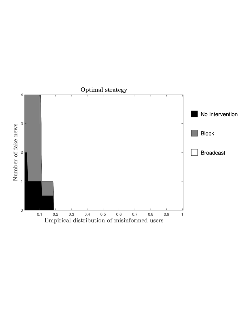
for any . It is desired to minimize the following cost function:
| (28) |
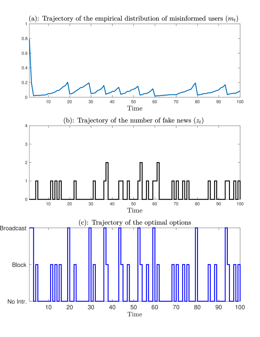
To determine the optimal strategy, we first compute the transition probability matrix in Theorem 1 and then solve the Bellman equation (11) in Theorem 2 by using the value-iteration method. The optimal strategy for is displayed in Figure 1 as a function of the empirical distribution of misinformed users and the number of fake news. Under this optimal strategy, one realization of Example 1 is depicted in Figure 2.
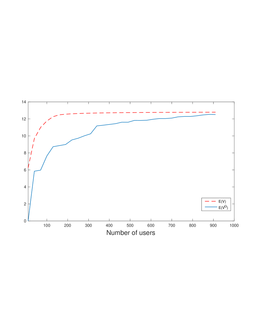
To verify the results of Theorem 3 and Corollary 1, let the Bellman equation (15) be quantized with a step size , and denote the resultant value function by , where is the closest number in to . Subsequently, it is shown in Figure 3 that converges to , as increases.
V Conclusions
A stochastic dynamic control strategy was introduced over a homogeneous network to minimize the spread of a persistent infection. It was shown that the exact optimal solution can be efficiently computed by solving a Bellman equation whose state space increases linearly with the number of nodes. In addition, an approximate optimal solution was proposed based on the infinite-population network, where the approximation error was shown to be upper bounded by a term that decays to zero as the number of users tends to infinity. An example of a social network was then presented to verify the theoretical results.
As a future research direction, the obtained results can be extended to partially homogeneous networks wherein the nodes are categorized into several sub-populations of homogeneous nodes such as low-degree and high-degree nodes. In addition, various approximation methods may be used to further alleviate the computational complexity of the proposed solutions. The development of reinforcement learning algorithms based on the Bellman equations provided in this paper can be another interesting problem for future work.
References
- [1] R. M. Anderson, The population dynamics of infectious diseases: Theory and applications. Springer, 2013.
- [2] O. Shy, “A short survey of network economics,” Review of Industrial Organization, vol. 38, no. 2, pp. 119–149, 2011.
- [3] G. A. Pagani and M. Aiello, “The power grid as a complex network: A survey,” Physica A: Statistical Mechanics and its Applications, vol. 392, no. 11, pp. 2688 –2700, 2013.
- [4] D. Easley and J. Kleinberg, Networks, crowds, and markets: Reasoning about a highly connected world. Cambridge University Press, 2010.
- [5] K. Sha, A. Striege, and M. Song, Security, Privacy and Reliability in Computer Communications and Networks. River Publishers, 2016.
- [6] I. Friedberg, F. Skopik, G. Settanni, and R. Fiedler, “Combating advanced persistent threats: From network event correlation to incident detection,” Computers & Security, vol. 48, pp. 35–57, 2015.
- [7] R. Pastor-Satorras, C. Castellano, P. Van Mieghem, and A. Vespignani, “Epidemic processes in complex networks,” Reviews of Modern Physics, vol. 87, no. 3, p. 925, 2015.
- [8] C. Nowzari, V. M. Preciado, and G. J. Pappas, “Analysis and control of epidemics: A survey of spreading processes on complex networks,” IEEE Control Systems, vol. 36, no. 1, pp. 26–46, 2016.
- [9] J. O. Kephart and S. R. White, “Directed-graph epidemiological models of computer viruses,” in Proceedings of IEEE Computer Society Symposium on Research in Security and Privacy, pp. 343–359, 1992.
- [10] M. Nekovee, Y. Moreno, G. Bianconi, and M. Marsili, “Theory of rumour spreading in complex social networks,” Physica A: Statistical Mechanics and its Applications, vol. 374, no. 1, pp. 457–470, 2007.
- [11] P. Van Mieghem, J. Omic, and R. Kooij, “Virus spread in networks,” IEEE/ACM Transactions on Networking, vol. 17, no. 1, pp. 1–14, 2009.
- [12] Y. Wang, D. Chakrabarti, C. Wang, and C. Faloutsos, “Epidemic spreading in real networks: An eigenvalue viewpoint,” in Proceedings of \nth22 IEEE International Symposium on Reliable Distributed Systems, pp. 25–34, 2003.
- [13] N. A. Ruhi and B. Hassibi, “SIRS epidemics on complex networks: Concurrence of exact markov chain and approximated models,” in Proceedings of the \nth54 IEEE Conference on Decision and Control, pp. 2919 – 2926, 2015.
- [14] R. Morton and K. H. Wickwire, “On the optimal control of a deterministic epidemic,” Advances in Applied Probability, vol. 6, no. 4, pp. 622–635, 1974.
- [15] A. Khanafer and T. Başar, “An optimal control problem over infected networks,” in Proceedings of the International Conference of Control, Dynamic Systems, and Robotics, Ottawa, Ontario, Canada, 2014.
- [16] S. Eshghi, M. Khouzani, S. Sarkar, and S. S. Venkatesh, “Optimal patching in clustered malware epidemics,” IEEE/ACM Transactions on Networking, vol. 24, no. 1, pp. 283–298, 2016.
- [17] A. Di Liddo, “Optimal control and treatment of infectious diseases. the case of huge treatment costs,” Mathematics, vol. 4, no. 2, p. 21, 2016.
- [18] C. Nowzari, V. M. Preciado, and G. J. Pappas, “Optimal resource allocation for control of networked epidemic models,” IEEE Transactions on Control of Network Systems, vol. 4, no. 2, pp. 159–169, 2017.
- [19] J. Arabneydi, “New concepts in team theory: Mean field teams and reinforcement learning,” Ph.D. dissertation, Dep. of Electrical and Computer Engineering, McGill University, Montreal, Canada, 2016.
- [20] J. Arabneydi and A. G. Aghdam, “A certainty equivalence result in team-optimal control of mean-field coupled Markov chains,” in Proceedings of the \nth56 IEEE Conference on Decision and Control, 2017, pp. 3125–3130.
- [21] ——, “Optimal dynamic pricing for binary demands in smart grids: A fair and privacy-preserving strategy,” in Proceedings of American Control Conference, 2018, pp. 5368–5373.
- [22] ——, “Near-optimal design for fault-tolerant systems with homogeneous components under incomplete information,” in Proceedings of the \nth61 IEEE International Midwest Symposium on Circuits and Systems, 2018, pp. 809–812.
- [23] J. Arabneydi, M. Baharloo, and A. G. Aghdam, “Optimal distributed control for leader-follower networks: A scalable design,” in Proceedings of the \nth31 IEEE Canadian Conference on Electrical and Computer Engineering, 2018, pp. 1–4.
- [24] M. Baharloo, J. Arabneydi, and A. G. Aghdam, “Near-optimal control strategy in leader-follower networks: A case study for linear quadratic mean-field teams,” in Proceedings of the \nth57 IEEE Conference on Decision and Control, 2018, pp. 3288–3293.
- [25] D. P. Bertsekas, Dynamic programming and optimal control. Athena Scientific, \nth4 Edition, 2012.