A monotone numerical integration method for mean-variance portfolio optimization under jump-diffusion models
Abstract
We develop a highly efficient, easy-to-implement, and strictly monotone numerical integration method for Mean-Variance (MV) portfolio optimization. This method proves very efficient in realistic contexts, which involve jump-diffusion dynamics of the underlying controlled processes, discrete rebalancing, and the application of investment constraints, namely no-bankruptcy and leverage.
A crucial element of the MV portfolio optimization formulation over each rebalancing interval is a convolution integral, which involves a conditional density of the logarithm of the amount invested in the risky asset. Using a known closed-form expression for the Fourier transform of this conditional density, we derive an infinite series representation for the conditional density where each term is strictly positive and explicitly computable. As a result, the convolution integral can be readily approximated through a monotone integration scheme, such as a composite quadrature rule typically available in most programming languages. The computational complexity of our proposed method is an order of magnitude lower than that of existing monotone finite difference methods. To further enhance efficiency, we propose an implementation of this monotone integration scheme via Fast Fourier Transforms, exploiting the Toeplitz matrix structure.
The proposed monotone numerical integration scheme is proven to be both -stable and pointwise consistent, and we rigorously establish its pointwise convergence to the unique solution of the MV portfolio optimization problem. We also intuitively demonstrate that, as the rebalancing time interval approaches zero, the proposed scheme converges to a continuously observed impulse control formulation for MV optimization expressed as a Hamilton-Jacobi-Bellman Quasi-Variational Inequality. Numerical results show remarkable agreement with benchmark solutions obtained through finite differences and Monte Carlo simulation, underscoring the effectiveness of our approach.
Keywords: mean-variance, portfolio optimization, monotonicity, numerical integration method, jump-diffusion, discrete rebalancing
1 Introduction
Long-term investors, such as holders of Defined Contribution plans, are typically motivated by asset allocation strategies which are optimal under multi-period criteria.111The holder of a Defined Contribution plan is effectively responsible to make investment decisions for both (i) the accumulation phase (pre-retirement) of about thirty years or more, and (ii) the decumulation phase (in retirement), of perhaps twenty years. As a result, multi-period portfolio optimisation plays a central role in asset allocation. In particular, originating with [47], mean-variance (MV) portfolio optimization forms the cornerstone of asset allocation ([24]), in part due to its intuitive nature which is the trade-off between risk (variance) and reward (mean). In multi-period settings, MV portfolio optimization aims to obtain an investment strategy (or control) that maximizes the expected value of the terminal wealth of the portfolio, for a given level of risk as measured by the associated variance of the terminal wealth [83]. In recent years, multi-period MV optimization has received considerable attention in in institutional settings, including in pension fund and insurance applications - see for example [32, 48, 40, 52, 64, 70, 75, 76, 79, 72, 29, 28, 11, 41, 78, 82, 85, 39], among many others.
It is important to distinguish between two categories of optimal investment strategies (optimal controls) for portfolio optimization. The first category, referred to as pre-commitment, typically results in time-inconsistent optimal strategies ([83, 37, 71, 20, 19]). The second category, namely the time-consistent or game theoretical approach, guarantees the time-consistency of the resulting optimal strategy by imposing a time-consistency constraint ([4, 6, 74, 12, 65]). The time-inconsistency of pre-commitment strategies is because the variance term in the MV-objective is not separable in the sense of dynamic programming (see [4, 71]). However, pre-commitment strategies are typically time-consistent under an alternative induced objective function [63], and hence implementable. The merits and demerits of time consistent and pre-commitment strategies are also discussed in [72]. In subsequent discussions, unless otherwise stated, both time consistent and pre-commitment strategies are collectively referred to strategies or controls.
1.1 Background
In the parametric approach, a parametric stochastic model is postulated, e.g. diffusion dynamics, and then is calibrated to market-observed data.222Recently, data-driven (i.e. non-parametric) methods have been proposed for portfolio optimization under different optimality criteria, including mean-variance [39, 10, 51]. Nonetheless, monotonicity of NN-based methods has not been established. A key concern about, and perhaps also a criticism against, MV portfolio optimization in a parametric setting is its potential lack of robustness to model misspecification error. This criticism originated from the fact that, in single-period settings, MV portfolio optimization can provide notoriously unstable asset allocation strategies arising from small changes in the underlying asset parameters ([50, 61, 54, 8]). Nonetheless, in the case of multi-period MV optimization, research findings indicate that, when the risky asset dynamics are allowed to follow pure-diffusion dynamics (e.g. GBM) or any of the standard finite-activity jump-diffusion models commonly encountered in financial settings, such as those considered in this work, the pre-commitment and time-consistent MV outcomes of terminal wealth are generally very robust to model misspecification errors [68].
It is well-documented in the finance literature that jumps are often present in the price processes of risky assets (see, for example, [15, 58]). In addition, findings in previous research work on MV portfolio optimization (pre-commitment and time-consistency strategies) also indicate that (i) jumps in the price processes of risky assets, such as Merton model [49] and the Kou model [36], and (ii) realistic investment constraints, such as no-bankruptcy or leverage, have substantial impact on efficient frontiers and optimal investment strategies of MV portfolio optimization [19, 65]. Furthermore, the results of [46] show that the effects of stochastic volatility, with realistic mean-reverting dynamics, are not important for long-term investors with time horizons greater than 10 years.
Furthermore, for multi-period MV optimization, it is documented in the literature that the composition of the risky asset basket remains relatively stable over time, which suggests that the primary question remains the overall risky asset basket vs. the risk-free asset composition of the portfolio, instead of the exact composition of the risky asset basket. See the available analytical solutions for multi-asset time-consistent MV problems (see, for example, [81]) as well as pre-commitment MV problems (see for example [37]). Therefore, it is reasonable to consider a well-diversified index, instead of a single stock or a basket of stocks, as common in the MV literature [66, 69, 68, 21, 67, 65]. This is the modeling approach adopted in this work, resulting in a low dimensional multi-period MV optimization problem.
1.1.1 Monotonicity and no-arbitrage
In general, since solutions to stochastic optimal control problems, including that of the MV portfolio optimization problem, are often non-smooth, convergence issues of numerical methods, especially monotonicity considerations, are of primary importance. This is because, in the context of numerical methods for optimal control problems, optimal decisions are determined by comparing numerically computed value functions. Non-monotone schemes could produce numerical solutions that fail to converge to financially relevant solution, i.e. a violation of the discrete no-arbitrage principle [53, 56, 77].
To illustrate the above point further, consider a generic time-advancement scheme from time-(-) to time- of the form
| (1.1) |
Here, are the weights and and is an index set typically capturing the computational stencil associated with the -th spatial partition point. This time-advancement scheme is monotone if, for any -th spatial partition point, we have , . Optimal controls at time- are determined typically by comparing candidates numerically computed from applying intervention on time-advancement results . Therefore, these candidates need to be approximated using a monotone scheme as well. If interpolation is needed in this step, linear interpolation is commonly chosen, due to its monotonicity333Other non-monotone interpolation schemes are discussed in, for example, [30, 59].. Loss of monotonicity occurring in the time-advancement may result in even for all .
1.1.2 Numerical methods
For stochastic optimal control problems with a small number of stochastic factors, the PDE approach is often a natural choice. To the best of our knowledge, finite difference (FD) methods remain the only pointwise convergent methods established for pre-commitment and time-consistent MV portfolio optimization in realistic investment scenarios. These scenarios involve the simultaneous application of various types of investment constraints and modeling assumptions, including jumps in the price processes of risky assets, as highlighted in [19, 65]. These FD methods achieve monotonicity in time-advancement through a positive coefficient finite difference discretization method (for the partial derivatives), which is combined with implicit time-stepping. Despite their effectiveness, finite difference methods present significant computational challenges in multi-period settings with long maturities. In particular, they necessitate time-stepping between rebalancing dates, which often occur annually (i.e., control monitoring dates). This time-stepping requirement introduces errors and substantially increase the computational cost of FD methods.
Fourier-based integration methods frequently rely on the presence of an analytical expression for the Fourier transform of the underlying transition density function, or an associated Green’s function, as highlighted in various research such as [45, 62, 2, 34, 26, 44, 43]. Notably, the Fourier cosine series expansion method [25, 60] can achieve high-order convergence for piecewise smooth problems. However, in cases of optimal control problems, which are usually non-smooth, such high-order convergence should not be anticipated.
When applicable, Fourier-based methods offer unique advantages over FD methods and Monte Carlo simulation. These advantages include the absence of timestepping errors between rebalancing (or control monitoring) dates, and the ability to handle complex underlying dynamics such as jump-diffusion, regime-switching, and stochastic variance in a straightforward manner. However, standard Fourier-based methods, much like Monte Carlo simulations, do have a significant drawback: they can potentially lose monotonicity. This potential loss of monotonicity in the context of variable annuities is discussed in depth in [34, 33].
In more detail, consider as the underlying (scaled) transition density, or a related Green’s function. For Lévy processes, which have independent and stationary increments, relies on and only through their difference, i.e., . Thus, the advancement of solutions between control monitoring dates takes the form of a convolution integral as follows
| (1.2) |
In the case of Lévy processes, even though is not known analytically, the Lévy-Khintchine formula provides an explicit representation of the Fourier transform (or the characteristic function) of , denoted by . This permits the use of Fourier series expansion to reconstruct the entire integral (1.2), not just the integrand. The approach creates a numerical integration scheme of the form (1.1), with the weights typically available in the Fourier domain via . Consequently, the algorithms boil down to the utilization of finite FFTs, which operate efficiently on most platforms. However, there is no assurance that the weights are non-negative for all and , which can potentially lead to a loss of monotonicity.
As highlighted in [3], the requirement for monotonicity in a numerical scheme can be relaxed. This notion of weak monotonicity was initially explored in [7] and was later examined in great detail in [26, 44, 43, 42] for general control problems in finance, including variable annuities. More specifically, the condition for monotonicity, i.e. for all , is relaxed to , with being a user-defined tolerance for monotonicity. By projecting the underlying transition density or an associated Green’s function onto linear basis functions, this approach allows for full control over potential monotonicity loss via the tolerance : the potential monotonicity loss can be quantified and restricted to , thereby enabling (pointwise) convergence as .
1.2 Objectives
In general, many industry practitioners find implementing monotone finite difference methods for jump-diffusion models to be complex and time-consuming, particularly when striving to utilize central differencing as much as possible, as proposed in [73]. As well-noted in the literature (e.g. [56, 59]), many seemingly reasonable finite difference discretization schemes can yield incorrect solutions. In addition, while the concept of (strict) monotonicity in numerical schemes is directly tied to the discrete no-arbitrage principle, making it easy to comprehend, weak monotonicity is less clear, which further hinders its application in practice. Moreover, the convergence analysis of weakly monotone schemes is often complex, potentially introducing additional obstacles to their practical application.
This paper aims to fill the aforementioned research gap through the development of an efficient, easy-to-implement and monotone numerical integration method for MV portfolio optimization under a realistic setting. This setting involves the simultaneous application of different types of investment constraints and jump-diffusion dynamics for the price processes of risky assets. In our method, the guarantee of the key monotonicity property comes with a trade-off: a modest level of analytical tractability is required for the jump sizes. Essentially, this stipulates that the associated jump-diffusion model should provide a closed-form expression for European vanilla options. This condition, however, conveniently accommodates a number of widely used models in finance, marking it as a relatively mild requirement in practice. To demonstrate this, we presents results for two popular distributions for jump sizes in finance: the normal distribution as put forth by [49], and the asymmetric double-exponential distribution as proposed in [36]. Although we focus on the pre-commitment strategy case, the proposed method can be extended to time-consistent MV optimization in a straightforward manner by enforcing a time-consistency constraint as in [65].
The main contributions of the paper are as follows.
-
(i)
We present a recursive and localized formulation of the pre-commitment MV portfolio optimization under a realistic context that involves the simultaneous application of different types of investment constraints and jump-diffusion dynamics [36, 49]. Over each rebalancing interval, the key component of the formulation of MV portfolio optimization is a convolution integral involving a conditional density of the logarithm of amount invested in the risky asset.
-
(ii)
Through a known closed-form expression of the Fourier transform of the underlying transition density, we derive an infinite series representation for this density in which all the terms of the series are non-negative and readily computable explicitly. Therefore, the convolution integral can be approximated in a straightforward manner using a monotone integration scheme via a composite quadrature rule. A significant benefit of the proposed method compared to existing monotone finite difference methods is that it offers a computational complexity that is an order of magnitude lower. Utilizing the Toeplitz matrix structure, we propose an efficient implementation of the proposed monotone integration scheme via FFTs.
-
(iii)
We mathematically demonstrate that the proposed monotone scheme is also -stable and pointwise consistent with the convolution integral formulation. We rigourously prove the pointwise convergence of the scheme as the discretization parameter approach zero. As the rebalancing time interval approaches zero, we intuitively demonstrate that the proposed scheme converges to a continuously observed impulse control formulation for MV optimization in the form of a Hamilton-Jacobi-Bellman Quasi-Variational Inequality.
-
(iv)
All numerical experiments are conducted using model parameters calibrated to inflation-adjusted, long-term US market data (89 years), enabling realistic conclusions to be drawn from the results. Numerical experiments demonstrate an agreement with benchmark results obtained by FD method and Monte Carlo simulation of [19].
Although we focus specifically on monotone integration methods for multi-period MV portfolio optimization, our comprehensive and systematic approach could serve as numerical and convergence analysis framework for the development of similar monotone integration methods for other multi-period or continuously observed control problems in finance.
In Section 2, we describe the underlying dynamics and a multi-period rebalancing framework for MV portfolio optimization. A localization of the pre-commitment MV portfolio optimization in the form of an convolution integral together with appropriate boundary conditions are presented in Section 3. Also therein, we present an infinite series representation of the transition density. A simple and easy-to-implement monotone numerical integration method via a composite quadrature rule is described in Section 4. In Section 5, we mathematically establish pointwise convergence the proposed integration method. Section 6 explore possible convergence between the proposed scheme and a Hamilton-Jacobi-Bellman Quasi-Variational Inequality arising from continuously observed impulse control formulation for MV optimization. Numerical results are given in Section 4. Section 8 concludes the paper and outlines possible future work.
2 Modelling
We consider portfolios consisting of a risk-free asset and a well-diversified stock index (the risky asset). With respect to the risk-free asset, we consider different lending and borrowing rates. Specifically, we denote by and the positive, continuously compounded rates at which the investor can respectively borrow funds or earn on cash deposits (with ). We make the standard assumption that the real world drift rate of the risky asset is strictly greater than . Since there is only one risky asset, with a constant risk-aversion parameter, it is never MV-optimal to short stock. Therefore, the amount invest in the risky-asset is non-negative for all , where denotes the fixed investment time horizon or maturity. In contrast, we do allow short positions in the risk-free asset, i.e. it is possible that the amount invested in the risk-free asset is negative. With this in mind, we denote by the time- amount invested in the risk-free asset and by the natural logarithm of the time- amount invested in the risky (so that is the amount).
For defining the jump-diffusion model dynamics, let be a random variable denoting the jump size. For any functional , we let and . Informally, (resp. ) denotes the instant of time immediately before (resp. after) the forward time . When a jump occurs, we have .
2.1 Discrete portfolio rebalancing
Define as the set of predetermined, equally spaced rebalancing times in ,
| (2.1) |
We adopt the convention that and the portfolio is not rebalanced at the end of the investment horizon . The evolution of the portfolio over a rebalancing interval , , can be viewed as consisting of three steps as follows. Over , , change according to some rebalancing strategy (i.e. an impulse control). Over the time period , there is no intervention by the investor according to some control (investment strategy), and therefore are uncontrolled, and are assumed to follow some dynamics for all . Over , the settlement (payment or receipt) of interest due for the time period . In the following, we first discuss stochastic modeling for over , then describe settlement of interest and modelling of rebalancing strategies using impulse controls.
Over the time period , in the absence of control (investor’s intervention according to some control strategy), the amounts in the risk-free and risky assets are assumed to have the following dynamics:
| (2.2) | |||||
Here, as noted earlier, and denote the positive, continuously compounded rates at which the investor can respectively borrow funds or earn on cash deposits (with ), while denotes the indicator function of the event ; is a standard Wiener process, and and are the real world drift rate and the instantaneous volatility, respectively. The jump term is a compound Poisson process. Specifically, is a Poisson process with a constant finite jump intensity ; and, with being a random variable representing the jump size, are independent and identically distributed (i.i.d.) random variables having the same same distribution as the random variable . In the dynamics (2.2), . Here, is the expectation operator taken under a suitable measure. The Poisson process , the sequence of random variables , and the Wiener process and are mutually independent.
We consider two distributions for the random variable , namely the normal distribution [49] and the asymmetric double-exponential distribution [36]. To this end, let be the probability density function (pdf) of . In the former case, , so that its pdf is given by
| (2.3) |
Also, in this case, , and hence can be computed accordingly. In the latter case, we consider an asymmetric double-exponential distribution for . Specifically, we consider , so that its pdf is given by
| (2.4) |
Here and respectively are the probabilities of upward and downward jump sizes. In this case, , so can be computed accordingly.
2.2 Impulse controls
Discrete portfolio rebalancing is modelled using the discrete impulse control formulation as discussed in for example [19, 65, 66], which we now briefly summarize below. Let denote the impulse applied at rebalancing time , which corresponds to the amount invested in the risk-free asset according to the investor’s intervention at time , and let denote the set of admissible impulse values, i.e. for all .
Let be the multi-dimensional underlying process, and denote the state of the system. Suppose that at time-, the state of the system is for some . We denote by the state of the system immediately after the application of the impulse at time , where
| (2.5) |
Here, is a fixed cost444It is straightforward to include a proportional cost into (2.5) as in [19]. However, to focus on the main advantages of the proposed method, we do not consider a proportional cost in this work.; since is undefined if , the amount becomes for a finite .
Associated with the fixed set of rebalancing times , defined in (2.1), an impulse control will be written as the set of impulse values
| (2.6) |
and we define to be the subset of the control applicable to the set of times ,
| (2.7) |
In a discrete setting, the amount invested in the risk-free asset changes only at rebalancing date. Specifically, over each time interval , we suppose the amount invested in the risk-free asset at time after rebalancing being . For test function with both and varying, we model the change in with for . Then, the amount in the risk-free asset would jump to at time , reflecting the settlement (payment or receipt) of interest due for the time interval , . Here, we note that, although there is no rebalancing at time , there is still settlement of interest for the interval .
2.3 Investment constraints
With the time- state of the system being , to include transaction cost, we define the liquidation value to be
| (2.8) |
We strictly enforce two realistic investment constraints on the joint values of and , namely a solvency condition and a maximum leverage condition. The solvency condition takes the following form: when , we require that the position in the risky asset be liquidated, the total remaining wealth be placed in the risk-free asset, and the ceasing of all subsequent trading activities. Specifically, assume that the system is in the state at time , where and
| (2.9) |
We define a solvency region and an insolvency or bankruptcy region as follows
| (2.10) |
The solvency constraint can then be stated as
| (2.11) |
where, as noted above, and is finite. This effectively means that the investment in the risky asset has to be liquidated, the total wealth is to be placed in the risk-free asset, and all subsequent trading activities much cease.
The maximum leverage constraint specifies that the leverage ratio after rebalancing at , where , is stipulated by (2.5) must satisfy
| (2.12) |
for some positive constant typically in the range . Given above the solvency constraint and the maximum leverage constraint, the set of admissible impulse values, namely the set is therefore defined as follows
Based on the definition (2.7), the set of admissible impulse controls is given by
| (2.13) |
3 Formulation
Let and respectively denote the mean and variance of the terminal liquidation wealth, given the system state at time for some following the control over , assuming the underlying dynamics (2.2). The standard scalarization method for multi-criteria optimization problem in [80] gives the mean-variance (MV) objective as
| (3.1) |
where the scalarization parameter reflects the investor’s risk aversion level.
3.1 Value function
Dynamic programming cannot be applied directly to (3.1), since no smoothing property of conditional expectation for variance. The technique of [38, 84] embeds (3.1) in a new optimisation problem, often referred to as the embedding problem, which is amenable to dynamic programming techniques. We follow the example of [13, 22] in defining the PCMV optimization problem as the associated embedding MV problem555For a discussion of the elimination of spurious optimization results when using the embedding formulation, see [23].. Specifically, with being the embedding parameter, we define the value function , as follows
| (3.2) |
where is given in (2.8), subject to dynamics (2.2) between rebalancing times. We denote by the optimal control for the problem , where
| (3.3) |
For an impulse value , we define the intervention operator applied at as follows
| (3.4) |
By dynamic programming arguments [55, 57], for a fixed embedding parameter , and , the recursive relationship for the value function in (3.2) is given by
| (3.5a) | ||||||
| (3.5b) | ||||||
| (3.5c) | ||||||
| (3.5d) | ||||||
Here, in (3.5b), the intervention operator is given by (3.4), with the operator reflecting the optimal choice between no-rebalancing and rebalancing (which is subject to a fixed cost ); (3.5c) reflects the settlement (payment or receipt) of interest due for the time interval , . In the integral (3.5d) the functions denotes the probability density of , the log of the amount invested in the risky asset at a future time (), and the information at the current time (), given . Also, we note that the fact that amount invested in the risk-free asset does not change in the in the interval is reflected in (3.5d) since this amount is kept constant () on both sides of (3.5d).
It can be shown that has the form , and therefore, in (3.5d), the integral takes the form of the convolution of and . That is, (3.5d) becomes
| (3.6) |
Although a closed-form expression for is not known to exist, its Fourier transform, denoted by , is known in closed-form. Specifically, we recall the Fourier transform pair
| (3.7) |
A closed-form expression for is given by
| (3.8) |
Here, , where is the probability density function of with being the random variable representing the jump multiplier.
3.2 An infinite series representation of
The proposed monotone integration method depends on an infinite series representation of the probability density function , which is presented in Lemma 3.1.
Lemma 3.1.
The infinite series representation in (3.9) cannot be applied directly for computation as the -th term of the series involves a multiple integral with , where denotes the probability density of . To feasibly evaluate this multiple integral analytically, as noted earlier, our method requires a quite modest level of analytical tractability for the random variable . To put it more precisely, we need the associated jump-diffusion model of the form to yield a closed-form expression for European vanilla options. Arguments in [17][Section 3.4.1] can be invoked to demonstrate this relationship. Thus, the requirement of analytical tractability for the random variable is not overly stringent, thereby broadening the applicability of our approach in practice.
Next, we demonstrate the applicability of our approach for two popular distributions for in finance: when follow a normal distribution [49] and an asymmetric double-exponential distribution [36].
Corollary 3.1.
Here, NorCDF denotes CDF of standard normal distribution . For brevity, we omit a straightforward proof for the log-normal case (3.10) using Equation (A.3). A proof for the log-double exponential case (3.1) is given in Appendix C. For this case, we note that function can be evaluated very efficiently using the standard normal density function and standard normal distribution function via the three-term recursion [1]
In the subsequent section, we present a definition of the localized problem to be solved numerically.
3.3 Localization and problem statement
The MV formulation (3.5) is posed on an infinite domain. For the problem statement and convergence analysis of numerical schemes, we define a localized MV portfolio optimsation formulation. To this end, with , , where , , , , and are sufficiently large, we define the following spatial sub-domains:
| (3.14) |
We emphasize that we do not actually solve the MV optimization problem in . However, we may use an approximate value to the solution in , obtained by means of extrapolation of the computed solution in , to provide any information required by the MV optimization problem in . We also define the following sub-domains:
| (3.15) |
The solutions within the sub-domains and are not required for our purposes. These sub-domains are introduced to ensure the well-defined computation of the conditional probability density function in (3.6) for the convolution integral (3.6) in the MV optimization problem within . To simplify our discussion, we will adopt a zero-padding convention going forward. This convention assumes that the value functions within these sub-domains are zero for all time , and we will exclude these sub-domains from further discussions.
Due to rebalancing, the intervention operator for , defined in (3.4), may require evaluating a candidate value at a point having , and could be outside , if . Therefore, with selected sufficiently large, we assume .
We now present equations for spatial sub-domains defined in (3.3). We note that boundary conditions for and are obtained by relevant asymptotic forms and , respectively, similar to [19]. This is detailed below.
-
•
For , we apply the terminal condition (3.5a)
(3.16) - •
-
•
For , , settlement of interest (3.5c) is enforced by
(3.18) -
•
For , where , we impose the boundary condition
(3.19) - •
-
•
For , where , from (3.16), for fixed , we assume that for some unknown function , which mimics asymptotic behaviour of the value function as (or equivalently, ). We substitute this asymptotic form into the integral (3.5d), noting the infinite series representation of given Lemma 3.1, and obtain the correspoding boundary condition:
(3.21) - •
In Definition 3.1 below, we formally define the MV portfolio optimization problem
Definition 3.1 (Localized MV portfolio optimization problem).
The MV portfolio optimization problem with the set of rebalancing times defined in (2.1), and dynamics (2.2) with the PDF given by (2.3) or (2.4), is defined in as follows.
At each , the solution to the MV portfolio optimization problem given by (3.17), where satisfies (i) the integral (3.22) in , (ii) the boundary conditions (3.20), (3.21), and (3.19) in , respectively, and (iii) subject to the terminal condition (3.16) in , with the settlement of interest subject to (3.18) in .
We introduce a result on uniform continuity of the solution to the MV portfolio optimization.
Proposition 3.1.
The solution to the MV portfolio optimization in Definition 3.1 is uniformly continuous within each sub-domain , .
Proof.
This proposition can be proved using mathematical induction on . For brevity, we outline key details below. We first note that the domain is bounded and is finite. We observe that if is a uniformly continuous function, then , where defined in (3.4), is also uniformly continuous [31, Lemma 2.2]. As such, is also uniformly continuous since is bounded. Therefore, it follows that if , is uniformly continuous then the intervention result obtained in (3.17) is also uniformly continuous. Next, if , , is uniformly continuous, then the interest settlement result defined in (3.18) is also uniformly continuous. The other key step is to show that, if , , is uniformly continuous, then the solution for given by the convolution integral (3.22) is also uniformly continuous. Combining these above three steps with the fact that the initial condition given in (3.16) is uniformly continuous in , with a bounded domain, gives the desired result. ∎
We conclude this section by emphasizing that the value function may not be continuous across and . The interior domain , , is the target region where provable pointwise convergence of the proposed numerical method is investigated, which relies on Proposition 3.1.
4 Numerical methods
Given the closed-form expressions of , the convolution integral (3.22) is approximated by a discrete convolution which can be efficiently computed via FFTs. For our scheme, the intervals and also serve as padding areas for nodes in . Without loss of generality, for convenience, we assume that and are chosen sufficiently large with
| (4.1) |
With this in mind, and , defined in (3.15), are given by
4.1 Discretization
We discretize MV portfolio optimization problem defined in Defn. 3.1 on the localized domain as follows.
-
(i)
We denote by (resp. and ) the number of intervals of a uniform partition of (resp. and ). For convenience, we typically choose and so that only one set of -coordinates is needed. We use an equally spaced partition in the -direction, denoted by , where
(4.2) -
(ii)
We use an unequally spaced partition in the -direction, denoted by , where , with , , , and .
We emphasize that no timestepping is required for the interval , . As noted earlier, is kept constant. We assume that there exists a discretization parameter such that
| (4.3) |
where the positive constants , , are independent of . For convenience, we occasionally use to refer to the reference gridpoint , , , . Nodes have (i) , in , (ii) , in , (iii) , in . and (iv) and , in padding sub-domains.
For , we denote by the exact solution at the reference node , where , and by the approximate solution at an arbitrary point obtained using the discretization parameter . We refer to the approximate solution at the reference node , where , as and . In the event that we need to evaluate at a point other than a node on the computational gridpoint, linear interpolation is used. We define by the discrete set of admissible impulse values defined as follows
| (4.4) |
where is defined in (2.3), and is the discretization parameter. With being an impulse value (a control), applying at the reference spatial node results in
| (4.5) |
For the special case , as discussed earlier, we only have interest rate payment, but no rebalancing, and therefore, only and are used.
4.2 Numerical schemes
For convenience, we define , and . Backwardly, over the time interval , , there are three key components solving the MV optimisation problem, namely (i) the interest settlement over as given in (3.18); (ii) the time advancement from to , as captured by (3.20)-(3.22), and (iii) the intervention action over as given in (3.17). We now propose the numerical schemes for these steps.
For , we impose the terminal condition (3.16) by
| (4.6) |
For imposing the intervention action (3.17), we solve the optimization problem
| (4.7) |
Here, is the approximate solution to the exact solution , where and is given by (2.5). The approximation is computed by linear interpolation as follows
| (4.8) |
Here, is a linear interpolation operator acting on the time- discrete solutions , and . We note that since , (4.8) boils down to a single dimensional interpolation along the -dimension.
Remark 4.1 (Attainability of local minima).
For the settlement of interest (3.18), linear interpolation/extrapolation is applied to compute as follows.
| (4.9) |
Here be linear interpolation/extrapolation operator acting on the time- discrete solutions , , where are given by (4.6) at and by (4.7) at . Note that when , becomes a linear extrapolation operator which imposes the boundary condition (3.19). That is,
| (4.10) |
For the time advancement of , . The boundary conditions, for as (3.20) and (3.21), can be imposed by
| (4.11) | |||||
| (4.12) |
In , we tackle the convolution integral in (3.22), where is fixed. For simplicity, we adopt the following notational convention: with and , we let , where is given by the infinite series (3.9). We also denote by an approximation to using the first terms of the infinite series (3.9). Applying the composite trapezoidal rule to approximate the convolution integral (3.22) gives the approximation in the form of a discrete convolution as follows
| (4.13) |
where are given in (4.9) and , , and .
Remark 4.2 (Monotonicity).
We highlight that the conditional density given by the infinite series (3.9) is defined and non-negative for all and (or, alternatively, for all and ). Therefore, scheme (4.13) is monotone.
We highlight that for computational purposes, , given by the infinite series (3.9), is truncated to . However, since each term of the series is non-negative, this truncation does not result in loss of monotonicity, which is a key advantage of the proposed approach.
As , there is no loss of information in the discrete convolution (4.13). For a finite , however, there is an error, namely , due to the use of a truncated Taylor series. Specifically, this truncation error can be bounded as follows:
| (4.14) |
Here, in (i), ; in (ii), . Therefore, from (4.14), as , we have , resulting in no loss of information. For a given , we can choose such that the error , for all and . This can be achieved by enforcing
| (4.15) |
It is straightforward to see that, if , then , as . For a given , we denote by be the smallest values that satisfies (4.15). We then have
| (4.16) |
This value can be obtained through a simple iterative procedure, as illustrated in Algorithm 4.1.
4.3 Efficient implementation and algorithms
In this section, we discuss an efficient implementation of the scheme presented above using FFT. For convenience, we define/recall sets of indices: , , , , with and . For brevity, we adopt the notational convention: for and , , where is chosen by (4.15). To effectively compute the discrete convolution in (4.13) for a fixed , we rewrite (4.13) in a matrix-vector product form as follows
| (4.17) |
Here, in (4.17), the vector is of size , the matrix is of size , and the vector is of size . It is important to note that is a Toeplitz matrix [9] having constant along diagonals. To compute the matrix-vector product in (4.17) efficiently using FFT, we take advantage of a cicular convolution product described below.
-
•
We first expand the non-square matrix (of size ) into a circulant matrix of size denoted by , and is defined as follows
(4.21) Here, , , , and are matrices of sizes , , , , and , respectively, and are given below
(4.26) (4.31) (4.36) (4.41) (4.46) -
•
For fixed , we construct a vector of size by augmenting vector , defined in (4.17), with zeros as follows
(4.47) Then, (4.17) can be implemented by applying a circulant matrix-vector product to compute an intermediate vector of discrete solutions as follows
(4.48) Here, the circulant matrix is given by (4.21), and the vector is given by (4.47), and the intermediate result is a vector of size , with is the middle (from the -th to the -th) elements of .
-
•
Observing that a circulant matrix-vector product is equal to a circular convolution product, (4.48) can further be written as a circular convolution product. More specifically, let be the first column of the circulant matrix defined in (4.21), and is given by
(4.49) The circular convolution product is defined componentwise by
where and are two sequences with the period (i.e. and , ). Then, (4.48) can be written as the following circular convolution product
(4.50) -
•
The circular convolution product in (4.50) can be computed efficiently using FFT and iFFT as follows
(4.51) -
•
Once the vector of intermediate discrete solutions is computed, we then obtain the vector of discrete solutions (of size ) for by discarding values , .
The implementation (4.51) suggests that we compute the weight components of only once, and reuse them for the computation over all time intervals. More specifically, for a given user-tolerance , using (4.15), we can compute a sufficiently large the number of terms in the infinite series representation (3.9) for these weights. Then, using Corollary 3.1, these weights for the case following a normal distribution [49] or a double-exponential distribution [36] can be computed only once in the Fourier space, as in (4.51), and reused for all time intervals. The step is described in Algorithm 4.1.
Putting everything together, in Algorithm 4.2, we present a monotone integration algorithm for MV portfolio optimization.
Remark 4.3 (Complexity).
Algorithm 4.2 involves, for , the key steps as follows.
-
•
Compute , , via FFT algorithm. The complexity of this step is , where we take into account (4.3).
-
•
We use exhaustive search through all admissible controls in to obtain global minimum. Each optimization problem is solved by evaluating the objective function times. There are nodes, and timesteps giving a total complexity . This is an order reduction compared to complexity of finite difference methods, which typically is for discrete rebalancing (see [19][Section 6.1].)
4.4 Construction of efficient frontier
We know discuss construction of efficient frontier. To this end, we define the auxiliary function , where , as defined in (3.3), is the optimal control for the problem obtained by solving the localized problem in Definition 3.1. Similar to [19, 66, 65], we now present a localized problem for , with and , in the sub-domains (3.3) as below
| (4.52a) | |||||
| (4.52b) | |||||
| (4.52c) | |||||
| (4.52d) | |||||
| (4.52e) | |||||
Here, in (4.52b), is the optimal impulse value obtained from solving the value function problem (3.17); (4.52c) is due to the settlement (payment or receipt) of interest due for the time interval , ; (4.52d)-(4.52e) are equations for spatial sub-domains , , and . The localized problem (4.52) can be solved numerically in a straightforward manner. In particular, at a reference gridpoint , the optimal impulse value in (4.52b) becomes which is the optimal impulse value obtained from Line (9) of Algorithm 4.2. We emphasize the convention that it may be non-optimal to rebalance, in which case, the convention is . Furthermore, the convolution integral in (4.52e) can be approximated using a scheme similar to (4.13). For brevity, we only provide the proof of numerical scheme for in Appendix B, and omit details of the other schemes for (4.52).
We assume that given the initial state at time and the positive discretization parameter , the efficient frontier (EF), denote by , can be traced out using the embedding parameter as below
| (4.53) |
Here, refers to a discretization approximation to the expression in the brackets. Specifically, for fixed , we let
| (4.54) |
Then and corresponding to in (4.53) are computed as follows
| (4.55) |
5 Pointwise convergence
In this section, we establish pointwise convergence of the proposed numerical integration method. We start by verifying three properties: -stability, monotonicity, and consistency (with respect to the integral formulation (3.22)). We recall that the infinite series is approximated by , where is an user-defined tolerance, and we have the error bound , as noted in (4.16).
It is straightforward to see that the proposed scheme is monotone since all the weights are positive. Therefore, we will primarily focus on -stability and consistency of the scheme. We will then show that convergence of our scheme is ensured if as , or equivalently, as .
For subsequent use, we present a remark about , , .
Remark 5.1.
Recalling that is a (conditional) probability density function, for a fixed , we have , hence . Furthermore, applying quadrature rule to approximate gives rise to an approximation error, denoted by , defined as follows
It is straightforward to see that as , i.e. as . Using the above results, recalling the weights , , are positive, and the error bound (4.16), we have
| (5.1) |
5.1 Stability
Our scheme consists of the following equations: (4.6) for , (4.11) for , (4.12) for , and finally (4.13) for . We start by verifying -stability of our scheme.
Lemma 5.1 (-stability).
Proof of Lemma 5.1.
First, we note that, for any fixed , as given by (4.6), and for a finite , we have , since is a bounded domain. Therefore, we have . Motivated by this observation, to demonstrate -stability of our scheme, we will show that, for a fixed , at any , , we have
| (5.2) |
where (i) is the error of the quadrature rule discussed in Remark 5.1, (ii) , and (iii) . In (5.2), the term is a result of the evaluation of using (4.10) for nodes near . For the rest of the proof, we will show the key inequality (5.2) when is fixed. The proof follows from a straightforward maximum analysis, since is a bounded domain. For brevity, we outline only key steps of an induction proof below.
We use induction , , to show the bound (5.2) for . For the base case, and thus (5.2) becomes
| (5.3) |
For the settlement of interest rate for all , as reflected by (4.9), we have , and . Since , it follows that
| (5.4) |
We now turn to -stability of (4.12) (for ). From (4.12), we note that for and ,
| (5.5) |
noting . Using (5.4), it is trivial that (4.11) (for ) satisfies
| (5.6) |
Now, we focus on the timestepping scheme (4.13) (for ). For and , we have
| (5.7) | ||||
| (5.8) |
Finally, given (5.8), we bound the intervention result , and , obtained from (4.7). Since linear interpolation is used, the weights for interpolation are non-negative. In addition, due to (5.5), (5.6), and (5.8), the numerical solutions at nodes used for interpolation, namely , , are also bounded by
Therefore, by monotonicity of linear interpolation, which is preserved by the operator in (4.7), , and , satisfy (5.3). We have proved the base case (5.3). Similar arguments can be used to show the induction step. This concludes the proof. ∎
5.2 Consistency
In this subsection, we mathematically demonstrate the pointwise consistency of the proposed scheme with respect to the MV optimization in Definition 3.1. Since it is straightforward that (4.6) is consistent with the terminal condition (3.16) (), we primarily focus on the consistency of the scheme on , .
We start by introducing notational convention. We use and , . In addition, for brevity, we use instead of , . We now write the MV portfolio optimization in Definition 3.1 and the proposed scheme in forms amendable for analysis. Recalling defined in (2.5), over each time interval , where , we write the MV portfolio optimization in Definition 3.1 via an operator as follows
| (5.9) |
Here, is given by
| (5.10a) | ||||
| (5.10b) | ||||
| (5.10c) | ||||
Similarly, the term in (5.2) is defined as follows
Next, we write the proposed scheme at , , in an equivalent form via an operator as follows
| (5.12) |
where
| (5.13a) | ||||
| (5.13b) | ||||
| (5.13c) | ||||
Similarly, the term in (5.12) is given by
We now introduce a lemma on local consistency of the proposed scheme.
Lemma 5.2 (Local consistency).
Suppose that (i) the discretization parameter satisfies (4.3), (ii) linear interpolation is used for the intervention action (4.7). For any smooth test function , with and , , and for a sufficiently small , we have
| (5.15) |
Here, as . The operators and are defined in (5.2) and (5.12), respectively, noting that depends on given in (5.13).
Proof of Lemma 5.2.
We first consider the operator defined in (5.13). For the case (5.13b) of (5.13), becomes
| (5.16) |
Here, (i) and (ii) are due to the facts that, for linear interpolation, the constant can be completely separated from interpolated values, and the interpolation error is of size for sufficiently small ; (iii) is due to (5.1) and being sufficiently small. The errors and in (iii) and (iv) are respectively described below.
- •
-
•
In (iv), is the error arising from the simple lhs numerical integration rule
(5.17) Due to the continuity and the boundedness of the integrand, we have as .
Since , is smooth, and is compact, for given in (5.16), we have
| (5.18) |
Next, similar to (5.13b), the term in (5.2) corresponding to is written as follows
| (5.19) |
Therefore, using (5.16), (5.2) and (5.18), and letting , for , the operator in (5.15) can be written as
| (5.20) |
which is (5.15) for , .
5.3 Main convergence theorem
Given the -stability and consistency of the proposed numerical scheme established in Lemmas 5.1 and 5.2, as well as together with its monotonicity, we now mathematically demonstrate the pointwise convergence of the scheme in , , as . Here, as noted earlier, we assume that as . We first need to recall/introduce relevant notation.
We denote by the computational grid parameterized by , noting that as . We also have the respective . In general, a generic gridpoint in , , is denoted by , whereas an arbitrary point in is denoted by . Numerical solutions at , , is denoted by , where it is emphasized that , which is the time- numerical solution at gridpoints is used for the computation of . The exact solution at an arbitrary point in , , is denoted by , where it is emphasized that , which is the time- exact solution in is used. More specifically, and are defined via operators and as follows
| (5.21) |
Here, our convention is that .
The pointwise convergence of the proposed scheme is stated in the main theorem below.
Theorem 5.1 (Pointwise convergence).
Proof of Theorem 5.1.
By Proposition 3.1, there exists (bounded) such that, for any ,
| (5.23) |
We then define
noting our convention that . To show (5.22), we will prove by mathematical induction on the following result: for any , and for sequence such that as ,
| (5.24) |
In the following proof, we let , , and be generic positive constants independent of and , which may take different values from line to line.
Base case : by (5.23), we can write . Therefore, by monotonicity of the scheme and (5.1), we have
| (5.25) |
Using (5.25) and the triangle inequality gives
| (5.26) |
By local consistency established in Lemma 5.2, we have
| (5.27) |
Due to smoothness of and regularity of , we have
| (5.28) |
Therefore, using (5.26), (5.27), (5.28), we can show that
| (5.29) | |||
noting as , and is bounded for all .
Induction hypothesis: assume that, for some , we have
| (5.30) |
Induction step: By the triangle inequality, we have
| (5.31) |
Now, we examine the first term (5.31). By the induction hypothesis (5.30), , where as . Therefore, the first term in (5.31) can be bounded by
| (5.32) |
Here, (i) follows from the local consistency of the numerical scheme established in Lemma 5.2. Next, we focus on the second term. Using the same arguments for the base case (see (5.29), with being replaced by ), the second term in (5.31) can be bounded by , where as . Here, we note that is bounded for all by Lemma 5.1 on stability. Combining this with (5.32), we have , where is bounded for all , and as . This concludes the proof. ∎
Remark 5.2 (Convergence on an infinite domain).
It is possible to develop a numerical scheme that converge to the solution of the theoretical formulation (3.5), in particular to the convolution integral (3.5d) which is posed on an infinite domain. This can be achieved by making a requirement on the discretization parameter (in addition to the assumption in (4.3)) as follows:
| (5.33) |
As such, as , we have (implying as well. It is straightforward to ensure (4.3) and (5.33) simultaneously as is being refined. For example, with , we can quadruple and sextuple as is being halved. Nonetheless, with and chosen sufficiently large as in our extensive experiments, numerical solutions in the interior () virtually do not get affected by the boundary conditions.
6 Continuously observed impulse control MV portfolio optimization
Recall that is the rebalancing time interval. In this section, we intuitively demonstrate that as , of the proposed numerical scheme converge to the viscosity solution [16, 3] of an impulse formulation of the continuously rebalanced MV portfolio optimization in [19]. A rigorous analysis of convergence to the viscosity solution of this impulse formulation is the topic of a paper in progress.
The impulse formulation proposed in [19] takes the form of an Hamilton-Jacobi-Bellman Quasi-Variational Inequality (HJB-QVI) as follows (boundary conditions omitted for brevity)
| (6.1a) | ||||
| (6.1b) | ||||
where and respectively are the differential and jump operators defined as follows
A -stable and consistent finite difference numerical scheme for the HJB-QVI (6.1) is presented in [19] in which monotonicity is ensured via a positive coefficient method. Therefore, convergence of this finite different scheme to the viscosity solution of the HJB-QVI is guaranteed [16, 3].
To intuitively see that the proposed scheme (5.12) is consistent in the viscosity sense with the impulse formulation (6.1) in , , we write (5.12) for via , where
| (6.2) |
where and are respectively given by
For a smooth test function , and a constant , term in (6.2) of are
| (6.3) |
Now, we first examine the term . Noting that
we have term- of (6.3)
| (6.4) |
Using similar techniques as in [44][Lemma 5.4], noting the it is possible to show that
| (6.5) |
By choosing , from (6.5), noting , the first term of (6.4) can be written as
| (6.6) |
The second term of (6.4) can be simplified as [44][Lemma 5.4]
| (6.7) |
Putting (6.6)-(6.7) into (6.4), noting that term- in (6.3) has the form , we have
| (6.8) |
Term in (6.2) can be handled using similar steps as in (5.16)-(5.18). Thus, (6.2) becomes
This show local consistency of the proposed scheme to (6.1a), that is,
| (6.9) |
Together with -stability and monotonicity of the proposed scheme, it is possible to utilize a Barles-Souganidis analysis [3] to show convergence to the viscosity solution of the impulse formulation (6.1) as . We leave this for our future work.
7 Numerical examples
7.1 Empirical data and calibration
In order to parameterize the underlying asset dynamics, the same calibration
data and techniques are used as detailed in [20, 27].
We briefly summarize the empirical data sources. The risky asset data
is based on daily total return data (including dividends and other
distributions) for the period 1926-2014 from the CRSP’s VWD index666Calculations were based on data from the Historical Indexes 2015©,
Center for Research in Security Prices (CRSP), The University of Chicago
Booth School of Business. Wharton Research Data Services was used
in preparing this article. This service and the data available thereon
constitute valuable intellectual property and trade secrets of WRDS
and/or its third party suppliers. , which is a capitalization-weighted index of all domestic stocks
on major US exchanges. The risk-free rate is based on 3-month US T-bill
rates777Data has been obtained from See http://research.stlouisfed.org/fred2/series/TB3MS.
over the period 1934-2014, and has been augmented with the NBER’s
short-term government bond yield data888Obtained from the National Bureau of Economic Research (NBER) website,
http://www.nber.org/databases/macrohistory/contents/chapter13.html. for 1926-1933 to incorporate the impact of the 1929 stock market
crash. Prior to calculations, all time series were inflation-adjusted
using data from the US Bureau of Labor Statistics999The annual average CPI-U index, which is based on inflation data for
urban consumers, were used - see http://www.bls.gov.cpi
..
In terms of calibration techniques, the calibration of the jump models is based on the thresholding technique of [15, 14] using the approach of [20, 27] which, in contrast to maximum likelihood estimation of jump model parameters, avoids problems such as ill-posedness and multiple local maxima101010If denotes the th inflation-adjusted, detrended log return in the historical risky asset index time series, a jump is identified in period if , where is an estimate of the diffusive volatility, is the time period over which the log return has been calculated, and is a threshold parameter used to identify a jump. For both the Merton and Kou models, the parameters in Table 7.2 is based on a value of , which means that a jump is only identified in the historical time series if the absolute value of the inflation-adjusted, detrended log return in that period exceeds 3 standard deviations of the “geometric Brownian motion change”, definitely a highly unlikely event. . In the case of GBM, standard maximum likelihood techniques are used. The calibrated parameters are provided in Table 7.2 (reproduced from [65, 66][Table 5.1]).
| Ref. level | -grid () | -grid () |
|---|---|---|
| 0 | 128 | 25 |
| 1 | 256 | 50 |
| 2 | 512 | 100 |
| 3 | 1024 | 200 |
| 4 | 2048 | 400 |
| Parameters | Merton | Kou |
|---|---|---|
| (drift) | 0.0817 | 0.0874 |
| (diffusion volatility) | 0.1453 | 0.1452 |
| (jump intensity) | 0.3483 | 0.3483 |
| (log jump multiplier mean) | -0.0700 | n/a |
| (log jump multiplier stdev) | 0.1924 | n/a |
| (probability of an up-jump) | n/a | 0.2903 |
| (exponential parameter up-jump) | n/a | 4.7941 |
| (exponential parameter down-jump) | n/a | 5.4349 |
| (borrowing interest rate) | 0.00623 | 0.00623 |
| (lending interest rate) | 0.00623 | 0.00623 |
For all experiments, unless otherwise noted, we use , and with the initial wealth being . We set , , , and , so that and .
For the user-defined tolerance used for the truncation of the infinite series representation of in (4.15), we use , which can be satisfied in discretely rebalancing examples when (i.e. the number terms in the truncated series of is 15).
7.2 Validation examples
Since for PCMV portfolio optimization under a solvency condition (no bankruptcy allowed) and a maximum leverage condition does not admit known analytical solution, we rely on existing numerical methods, namely (i) finite difference [19, 21] and (ii) Monte Carlo (MC) simulation to verify results. For brevity, we will refer to the proposed monotone integration method as the “MI” method, and to the finite difference method of [19, 21] as the “FD” method.
As noted earlier, to the best of our knowledge, the FD methods proposed in [19, 21] are the only existing FD methods for MV optimization under jump-diffusion dynamics with investment constraints. In discrete rebalancing setting, FD methods typically involve solving, between two consecutive rebalancing times, a Partial Integro Differential Equation (PIDE), where the amount invested in the risky asset is the independent variable. These FD methods achieve monotonicity in time-advancement through a positive coefficient finite difference discretization method (for the partial derivatives), which is combined with implicit timestepping. Optimal strategies are obtained by solving an optimization problem across rebalancing times. Despite their effectiveness, finite difference methods present significant computational challenges in multi-period settings with very long maturities, as encountered in DC plans. In particular, they necessitate time-stepping between rebalancing dates (i.e., control monitoring dates), which often occur annually. This time-stepping requirement introduces errors and substantially increase the computational cost of FD methods (as noted earlier in Remark 4.3. In the numerical experiments, the FD results are obtained on the same computational domain as those obtained by the MI method with the number of partition points in the - and -grids being and , respectively, with 256 timesteps between yearly rebalancing times. (This approximates to a daily timestepping.)
Validation against MC simulation is proceeded in two steps. In Step 1, we solve the PCMV problem using the MI method on a relatively fine computational grid: the number of partition points in the - and -grids are and , respectively. During this step, the optimal controls are stored for each discrete state value and rebalancing time . In Step 2, we carry out Monte Carlo simulations with paths from to following these stored numerical optimal strategies for asset allocation across each , using linear interpolation, if necessary, to determine the controls for a given state value. For Step 2, an Euler’s timestepping method is used for timestepping between consecutive rebalancing times and we use a total of timesteps.
7.2.1 Discrete rebalancing
For discretely rebalancing experiments, we use (years), with year (yearly rebalancing). The the details of the mesh size/timestep refinement level used are given in Table 7.1.
Table 7.3 presents the numerically computed and under the Kou model obtained for different refinement levels with and and (years). To provide an estimate of the convergence rate of the proposed MI method, we compute the “Change” as the difference in values from the coarser grid and the “Ratio” as the ratio of changes between successive grids. For validation purposes, and obtained by FD method, as well as those obtained by MC methods, together with 95% confidence intervals (CIs), are also provided. As evident from Table 7.3, means and standard deviations obtained by the MI method exhibit excellent agreement with those obtained by the FD method and MC simulation.
Results obtained by MC simulation agree with those obtained by our numerical method. Results for the Merton jump case when and (years) are presented in Table 7.4 and similar observations can be made.
| Method | Ref. level | Change | Ratio | Change | Ratio | |||
| MI | ||||||||
| 20 | ||||||||
| (years) | MC | |||||||
| CI | ||||||||
| FD | ||||||||
| MI | ||||||||
| 30 | ||||||||
| (years) | MC | |||||||
| CI | ||||||||
| FD | ||||||||
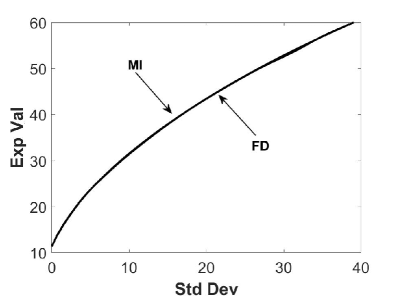
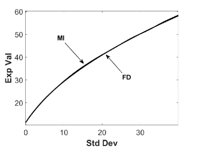
In Figure 7.1 presents we present efficient frontiers for the Merton model (Figure 7.1 (a)) and for the Kou model (Figure 7.1 (b)) obtained by the MI’s methods with refinement level ( and ). We observe that efficient frontiers produced by the MI’s method agree well with those obtained by the FD method.
| Method | Ref. level | Change | Ratio | Change | Ratio | |||
| MI | ||||||||
| 20 | ||||||||
| (years) | MC | |||||||
| CI | ||||||||
| FD | 73.9518 | 46.5288 | ||||||
| MI | ||||||||
| 30 | ||||||||
| (years) | MC | |||||||
| CI | ||||||||
| FD | 93.6812 | 41.7168 | ||||||
7.2.2 Continuous rebalancing
While continuous rebalancing is not the primary focus of this paper, we believe it is valuable to include numerical results for the continuous rebalancing setting in order to validate the method. For experiments in the continuous rebalancing setting, we use (years), with year. The details of the mesh size/timestep refinement level used are given in Table 7.5. The model parameters, according to [19], are given in Table 7.6.
In these experiments, we also consider the scenario where the dynamics of the risky asset follow a Geometric Brownian Motion (GBM) model. In cases where pure diffusion is desired, such as in a GBM model, the occurrence of jumps can be eliminated by setting . Table 7.7 displays the numerical results for (expected value) and (standard deviation) obtained at various refinement levels. These results correspond to the case where and years, assuming a GBM model. For validation purposes, we also include the expected values and standard deviations obtained using the FD method proposed by [19]. The results are presented alongside the values obtained through the proposed MI method in Table 7.7. Notably, it is evident from the table that the FD and MI results show excellent agreement.
| Ref. level | Timesteps | -grid | -grid |
|---|---|---|---|
| 0 | 10 | 128 | 25 |
| 1 | 20 | 256 | 50 |
| 2 | 40 | 512 | 100 |
| 3 | 80 | 1024 | 200 |
| 4 | 160 | 2048 | 400 |
| Parameters | GBM | Merton |
|---|---|---|
| (drift) | 0.15 | 0.0795487 |
| (diffusion volatility) | 0.15 | 0.1765 |
| (jump intensity) | n/a | 0.0585046 |
| (log jump multiplier mean) | n/a | -0.788325 |
| (log jump multiplier stdev) | n/a | 0.450500 |
| (borrowing interest rate) | 0.04 | 0.0445 |
| (lending interest rate) | 0.04 | 0.0445 |
| Method | Ref. level | Change | Ratio | Change | Ratio | ||
|---|---|---|---|---|---|---|---|
| MI | |||||||
| FD | 38.4789 | 5.0888 | |||||
| Method | Ref. level | Change | Ratio | Change | Ratio | ||
|---|---|---|---|---|---|---|---|
| MI | |||||||
| FD | 24.6032 | 22.2024 | |||||
8 Conclusion
In this study, we present a highly efficient, straightforward-to-implement, and monotone numerical integration method for MV portfolio optimization. The model considered in this paper addresses a practical context that includes a variety of investment constraints, as well as jump-diffusion dynamics that govern the price processes of risky assets. Our method employs an infinite series representation of the transition density, wherein all series terms are strictly positive and explicitly computable. This approach enables us to approximate the convolution integral for time-advancement over each rebalancing interval via a monotone integration scheme. The scheme uses a composite quadrature rule, simplifying the computation significantly. Furthermore, we introduce an efficient implementation of the proposed monotone integration scheme using FFTs, exploiting the structure of Toeplitz matrices. The pointwise convergence of this scheme, as the discretization parameter approaches zero, is rigorously established. Numerical experiments affirm the accuracy of our approach, aligning with benchmark results obtained through the FD method and Monte Carlo simulation, as demonstrated in [19]. Notably, our proposed method offers superior efficiency compared to existing FD methods, owing to its computational complexity being an order of magnitude lower.
Further work includes investigation of self-exciting jumps for MV optimization, together with a convergence analysis as to a continuously observed impulse control formulation for MV optimization taking the form of a HJB Quasi-Variational Inequality.
References
- [1] M. Abramowitz and I. A. Stegun. Handbook of mathematical functions. Dover, New York, 1972.
- [2] J. Alonso-Garcca, O. Wood, and J. Ziveyi. Pricing and hedging guaranteed minimum withdrawal benefits under a general Lévy framework using the COS method. Quantitative Finance, 18:1049–1075, 2018.
- [3] G. Barles and P.E. Souganidis. Convergence of approximation schemes for fully nonlinear equations. Asymptotic Analysis, 4:271–283, 1991.
- [4] S. Basak and G. Chabakauri. Dynamic mean-variance asset allocation. Review of Financial Studies, 23:2970–3016, 2010.
- [5] Edouard Berthe, Duy-Minh Dang, and Luis Ortiz-Gracia. A shannon wavelet method for pricing foreign exchange options under the heston multi-factor cir model. Applied Numerical Mathematics, 136:1–22, 2019.
- [6] T. Björk and A. Murgoci. A theory of Markovian time-inconsistent stochastic control in discrete time. Finance and Stochastics, (18):545–592, 2014.
- [7] O. Bokanowski, A. Picarelli, and C. Reisinger. High-order filtered schemes for time-dependent second order HJB equations. ESAIM Mathematical Modelling and Numerical Analysis, 52:69–97, 2018.
- [8] T. Bourgeron, E. Lezmi, and T. Roncalli. Robust asset allocation for robo-advisors. Working paper, 2018.
- [9] Wlodzimierz Bryc, Amir Dembo, and Tiefeng Jiang. Spectral measure of large random hankel, markov and toeplitz matrices. Annals of probability, 34(1):1–38, 2006.
- [10] Andrew Butler and Roy H Kwon. Data-driven integration of regularized mean-variance portfolios. arXiv preprint arXiv:2112.07016, 2021.
- [11] Z. Chen, G. Li, and J. Guo. Optimal investment policy in the time consistent mean–variance formulation. Insurance: Mathematics and Economics, 52(2):145–156, March 2013.
- [12] F. Cong and C.W. Oosterlee. On pre-commitment aspects of a time-consistent strategy for a mean-variance investor. Journal of Economic Dynamics and Control, 70:178–193, 2016.
- [13] F Cong and CW Oosterlee. On robust multi-period pre-commitment and time-consistent mean-variance portfolio optimization. International Journal of Theoretical and Applied Finance, 20(07):1750049, 2017.
- [14] R. Cont and C. Mancini. Nonparametric tests for pathwise properties of semi-martingales. Bernoulli, (17):781–813, 2011.
- [15] R. Cont and P. Tankov. Financial modelling with jump processes. Chapman and Hall / CRC Press, 2004.
- [16] M. G. Crandall, H. Ishii, and P. L. Lions. User’s guide to viscosity solutions of second order partial differential equations. Bulletin of the American Mathematical Society, 27:1–67, 1992.
- [17] D. M. Dang, K. R. Jackson, and S. Sues. A dimension and variance reduction Monte Carlo method for pricing and hedging options under jump-diffusion models. Applied Mathematical Finance, 24:175–215, 2017.
- [18] D. M. Dang and Luis Ortiz-Gracia. A dimension reduction Shannon-wavelet based method for option pricing. Journal of Scientific Computing, 2017. https://doi.org/10.1007/s10915-017-0556-y.
- [19] D.M. Dang and P.A. Forsyth. Continuous time mean-variance optimal portfolio allocation under jump diffusion: A numerical impulse control approach. Numerical Methods for Partial Differential Equations, 30:664–698, 2014.
- [20] D.M. Dang and P.A. Forsyth. Better than pre-commitment mean-variance portfolio allocation strategies: A semi-self-financing Hamilton–Jacobi–Bellman equation approach. European Journal of Operational Research, (250):827–841, 2016.
- [21] D.M. Dang, P.A. Forsyth, and K.R. Vetzal. The 4 percent strategy revisited: a pre-commitment mean-variance optimal approach to wealth management. Quantitative Finance, 17(3):335–351, 2017.
- [22] Duy-Minh Dang and Peter A Forsyth. Continuous time mean-variance optimal portfolio allocation under jump diffusion: An numerical impulse control approach. Numerical Methods for Partial Differential Equations, 30(2):664–698, 2014.
- [23] Duy-Minh Dang, Peter A Forsyth, and Yuying Li. Convergence of the embedded mean-variance optimal points with discrete sampling. Numerische Mathematik, 132(2):271–302, 2016.
- [24] E.J. Elton, M.J. Gruber, S.J. Brown, and W.N. Goetzmann. Modern portfolio theory and investment analysis. Wiley, 9th edition, 2014.
- [25] F. Fang and C.W. Oosterlee. A novel pricing method for European options based on Fourier-Cosine series expansions. SIAM Journal on Scientific Computing, 31:826–848, 2008.
- [26] P. A. Forsyth and G. Labahn. -monotone Fourier methods for optimal stochastic control in finance. 2017. Working paper, School of Computer Science, University of Waterloo.
- [27] P.A. Forsyth and K.R. Vetzal. Dynamic mean variance asset allocation: Tests for robustness. International Journal of Financial Engineering, 4:2, 2017. 1750021 (electronic).
- [28] P.A. Forsyth and K.R. Vetzal. Optimal asset allocation for retirement saving: Deterministic vs. time consistent adaptive strategies. Applied Mathematical Finance, 26(1):1–37, 2019.
- [29] P.A. Forsyth, K.R. Vetzal, and G. Westmacott. Management of portfolio depletion risk through optimal life cycle asset allocation. North American Actuarial Journal, 23(3):447–468, 2019.
- [30] F. N. Fritsch and R. E. Carlson. Monotone piecewise cubic interpolation. SIAM Journal on Numerical Analysis, 17:238–246, 1980.
- [31] X. Guo and G. Wu. Smooth fit principle for impulse control of multidimensional diffusion processes. SIAM Journal on Control and Optimization, 48(2):594–617, 2009.
- [32] B. Hojgaard and E. Vigna. Mean-variance portfolio selection and efficient frontier for defined contribution pension schemes. Research Report Series, Department of Mathematical Sciences, Aalborg University, R-2007-13, 2007.
- [33] Y.T. Huang and Y.K. Kwok. Regression-based Monte Carlo methods for stochastic control models: variable annuities with lifelong guarantees. Quantitative Finance, 16(6):905–928, 2016.
- [34] Y.T. Huang, P. Zeng, and Y.K. Kwok. Optimal initiation of guaranteed lifelong withdrawal benefit with dynamic withdrawals. SIAM Journal on Financial Mathematics, 8:804–840, 2017.
- [35] S. G. Kou. A jump diffusion model for option pricing. Management Science, 48:1086–1101, August 2002.
- [36] S.G. Kou. A jump-diffusion model for option pricing. Management Science, 48(8):1086–1101, 2002.
- [37] D. Li and W.-L. Ng. Optimal dynamic portfolio selection: multi period mean variance formulation. Mathematical Finance, 10:387–406, 2000.
- [38] D. Li and W.L. Ng. Optimal Dynamic Portfolio Selection: Multiperiod Mean-Variance Formulation. Mathematical Finance, 10(3):387–406, 2000.
- [39] Y. Li and P.A. Forsyth. A data-driven neural network approach to optimal asset allocation for target based defined contribution pension plans. Insurance: Mathematics and Economics, (86):189–204, 2019.
- [40] X. Liang, L. Bai, and J. Guo. Optimal time-consistent portfolio and contribution selection for defined benefit pension schemes under mean-variance criterion. ANZIAM, (56):66–90, 2014.
- [41] X. Lin and Y. Qian. Time-consistent mean-variance reinsurance-investment strategy for insurers under cev model. Scandinavian Actuarial Journal, (7):646–671, 2016.
- [42] Y. Lu and D.M. Dang. A pointwise convergent numerical integration method for Guaranteed Lifelong Withdrawal Benefits under stochastic volatility.
- [43] Y. Lu and D.M. Dang. A semi-Lagrangian -monotone Fourier method for continuous withdrawal GMWBs under jump-diffusion with stochastic interest rate.
- [44] Y. Lu, D.M. Dang, P.A. Forsyth, and G. Labahn. An -monotone Fourier method for Guaranteed Minimum Withdrawal Benefit (GMWB) as a continuous impulse control problem.
- [45] X. Luo and P.V. Shevchenko. Valuation of variable annuities with guaranteed minimum withdrawal and death benefits via stochastic control optimization. Insurance: Mathematics and Economics, 62(3):5–15, 2015.
- [46] K. Ma and P. A. Forsyth. Numerical solution of the Hamilton-Jacobi-Bellman formulation for continuous time mean variance asset allocation under stochastic volatility. Journal of Computational Finance, 20(01):1–37, 2016.
- [47] H. Markowitz. Portfolio selection. The Journal of Finance, 7(1):77–91, March 1952.
- [48] F. Menoncin and E. Vigna. Mean-variance target-based optimisation in DC plan with stochastic interest rate. Working paper, Collegio Carlo Alberto, (337), 2013.
- [49] R.C. Merton. Option pricing when underlying stock returns are discontinuous. Journal of Financial Economics, 3:125–144, 1976.
- [50] R.O. Michaud and R.O. Michaud. Efficient asset management: A practical guide to stock portfolio optimization and asset allocation. Oxford University Press, 2 edition, 2008.
- [51] Chendi Ni, Yuying Li, Peter Forsyth, and Ray Carroll. Optimal asset allocation for outperforming a stochastic benchmark target. Quantitative Finance, 22(9):1595–1626, 2022.
- [52] C.I. Nkeki. Stochastic funding of a defined contribution pension plan with proportional administrative costs and taxation under mean-variance optimization approach. Statistics, optimization and information computing, (2):323–338, 2014.
- [53] A.M. Oberman. Convergent difference schemes for degenerate elliptic and parabolic equations: Hamilton–Jacobi Equations and free boundary problems. SIAM Journal Numerical Analysis, 44(2):879–895, 2006.
- [54] S. Perrin and T. Roncalli. Machine Learning Optimization Algorithms and Portfolio Allocation, chapter 8, pages 261–328. Wiley Online Library, 2020.
- [55] H. Pham. On some recent aspects of stochastic control and their applications. Probability Surveys, 2:506–549, 2005.
- [56] D.M. Pooley, P.A. Forsyth, and K.R. Vetzal. Numerical convergence properties of option pricing PDEs with uncertain volatility. IMA Journal of Numerical Analysis, 23:241–267, 2003.
- [57] M. Puterman. Markov Decison Processes: Discrete Stochastic Dynamic Programming. Wiley, New York, 1994.
- [58] C. Ramezani and Y. Zeng. Maximum likelihood estimation of the double exponential jump-diffusion process. Annals of Finance, 3(4):487–507, 2007.
- [59] C. Reisinger and P.A. Forsyth. Piecewise constant Policy approximations to Hamilton-Jacobi-Bellman equations. Applied Numerical Mathematics, 103:27–47, 2016.
- [60] M.J. Ruijter, C.W. Oosterlee, and R.F.T. Aalbers. On the Fourier cosine series expansion (COS) method for stochastic control problems. Numerical Linear Algebra with Applications, 20:598–625, 2013.
- [61] Y. Sato. Model-free reinforcement learning for financial portfolios: A brief survey. Working paper, 2019.
- [62] P.V. Shevchenko and X. Luo. A unified pricing of variable annuity guarantees under the optimal stochastic control framework. Risks, 4(3):1–31, 2016.
- [63] M. Strub, D. Li, and X. Cui. An enhanced mean-variance framework for robo-advising applications. SSRN 3302111, 2019.
- [64] J. Sun, Z. Li, and Y. Zeng. Precommitment and equilibrium investment strategies for defined contribution pension plans under a jump–diffusion model. Insurance: Mathematics and Economics, (67):158–172, 2016.
- [65] P. M. Van Staden, D.M. Dang, and P.A. Forsyth. Time-consistent mean-variance portfolio optimization: a numerical impulse control approach. Insurance: Mathematics and Economics, 83(C):9–28, 2018.
- [66] P. M. Van Staden, D.M. Dang, and P.A. Forsyth. Mean-quadratic variation portfolio optimization: A desirable alternative to time-consistent mean-variance optimization? SIAM Journal on Financial Mathematics, 10(3):815–856, 2019.
- [67] P. M. Van Staden, D.M. Dang, and P.A. Forsyth. On the distribution of terminal wealth under dynamic mean-variance optimal investment strategies. SIAM Journal on Financial Mathematics, 12(2):566–603, 2021.
- [68] P. M. Van Staden, D.M. Dang, and P.A. Forsyth. The surprising robustness of dynamic mean-variance portfolio optimization to model misspecification errors. European Journal of Operational Research, 289:774–792, 2021.
- [69] Pieter M Van Staden, Duy-Minh Dang, and Peter A Forsyth. Practical investment consequences of the scalarization parameter formulation in dynamic mean–variance portfolio optimization. International Journal of Theoretical and Applied Finance, 24(05):2150029, 2021.
- [70] E. Vigna. On efficiency of mean-variance based portfolio selection in defined contribution pension schemes. Quantitative Finance, 14(2):237–258, 2014.
- [71] E. Vigna. On time consistency for mean-variance portfolio selection. International Journal of Theoretical and Applied Finance, 23(6), 2020.
- [72] Elena Vigna. Tail optimality and preferences consistency for intertemporal optimization problems. SIAM Journal on Financial Mathematics, 13(1):295–320, 2022.
- [73] J. Wang and P.A. Forsyth. Maximal use of central differencing for Hamilton-Jacobi-Bellman PDEs in finance. SIAM Journal on Numerical Analysis, 46:1580–1601, 2008.
- [74] J. Wang and P.A. Forsyth. Continuous time mean variance asset allocation: A time-consistent strategy. European Journal of Operational Research, 209(2):184–201, 2011.
- [75] L. Wang and Z. Chen. Nash equilibrium strategy for a DC pension plan with state-dependent risk aversion: A multiperiod mean-variance framework. Discrete Dynamics in Nature and Society, (1-17), 2018.
- [76] L. Wang and Z. Chen. Stochastic game theoretic formulation for a multi-period DC pension plan with state-dependent risk aversion. Mathematics, 7(108):1–16, 2019.
- [77] Xavier Warin. Some non-monotone schemes for time dependent Hamilton-Jacobi-Bellman equations in stochastic control. Journal of Scientific Computing, 66(3):1122–1147, 2016.
- [78] J. Wei and T. Wang. Time-consistent mean-variance asset-liability management with random coefficients. Insurance: Mathematics and Economics, (77):84–96, 2017.
- [79] H. Wu and Y. Zeng. Equilibrium investment strategy for defined-contribution pension schemes with generalized mean-variance criterion and mortality risk. Insurance: Mathematics and Economics, 64:396–408, 2015.
- [80] P Le Yu. Cone convexity, cone extreme points, and nondominated solutions in decision problems with multiobjectives. Journal of Optimization Theory and Applications, 14(3):319–377, 1974.
- [81] Y. Zeng and Z. Li. Optimal time-consistent investment and reinsurance policies for mean-variance insurers. Insurance: Mathematics and Economics, 49(1):145–154, July 2011.
- [82] H. Zhao, Y. Shen, and Y. Zeng. Time-consistent investment-reinsurance strategy for mean-variance insurers with a defaultable security. Journal of Mathematical Analysis and Applications, 437(2):1036–1057, May 2016.
- [83] X. Zhou and D. Li. Continuous time mean variance portfolio selection: a stochastic LQ framework. Applied Mathematics and Optimization, 42:19–33, 2000.
- [84] X.Y. Zhou and D. Li. Continuous-time mean-variance portfolio selection: A stochastic LQ framework. Applied Mathematics and Optimization, 42(1):19–33, 2000.
- [85] Z. Zhou, H. Xiao, J. Yin, X. Zeng, and L. Lin. Pre-commitment vs. time-consistent strategies for the generalized multi-period portfolio optimization with stochastic cash flows. Insurance: Mathematics and Economics, (68):187–202, 2016.
Appendices
Appendix A Proof of Lemma 3.1
Recalling the inverse Fourier transform in (3.7) and the closed-form expression for in (3.8), we have
| (A.1) |
where , and are given in (3.9), and . Following the approach developed in [17, 18, 5] , we expand the term in (A.1) in a Taylor series, noting that
| (A.2) |
where is the probability density of , and , with , and for , . Then, we have
| (A.3) | |||||
| (A.4) |
where the first term of the series corresponds to and is equal to . Here, in (i), we use the Fubini’s theorem and the well known result .
Appendix B : boundary expressions
Recalling the sub-domain definitions in (3.3), we observe that is the boundary where . For fixed , noting the terminal condition (3.16), we assume that for some unknown function . Using the infinite series representation of given Lemma 3.1 (proof in Appendix A) and the integral (3.5d), we have
where we use , and .
Similarly, for each fixed , we assume the auxiliary linear value function , for some unknown function . we have
Appendix C Proof of for
In this case, according to Lemma 3.1, we have
| (C.1) |
Here, the term in (C.1) is clearly non-negative and can be computed as
| (C.2) |
where is the PDF of the random variable , for fixed . To find , the key step is the decomposition of into sums of i.i.d exponential random variables [35]. More specifically, we have
| (C.3) |
Here, and are given in (3.1), and and are i.i.d. exponential variables with rates and , respectively. The PDF for each of the cases in (C.3) respectively are
| (C.4) |
Taking into account (C.3)-(C.4), (C.2) becomes
| (C.5) |
Considering the term ,
Making the change of variable ,
Making the change of variable ,
| (C.6) | ||||
where is defined in (3.13). Similarly for the term ,
| (C.7) | ||||
where is defined in (3.13). Using (C.5), (C.6) and (C.7) together with further simplifications gives us (3.1).