A multinode quantum network over a metropolitan area
Abstract
Towards realizing the future quantum internet, a pivotal milestone entails the transition from two-node proof-of-principle experiments conducted in laboratories to comprehensive, multi-node setups on large scales. Here, we report on the debut implementation of a multi-node entanglement-based quantum network over a metropolitan area. We equipped three quantum nodes with atomic quantum memories and their telecom interfaces, and combined them into a scalable phase-stabilized architecture through a server node. We demonstrated heralded entanglement generation between two quantum nodes situated 12.5 km apart, and the storage of entanglement exceeding the round-trip communication time. We also showed the concurrent entanglement generation on three links. Our work provides a metropolitan-scale testbed for the evaluation and exploration of multi-node quantum network protocols and starts a new stage of quantum internet research.
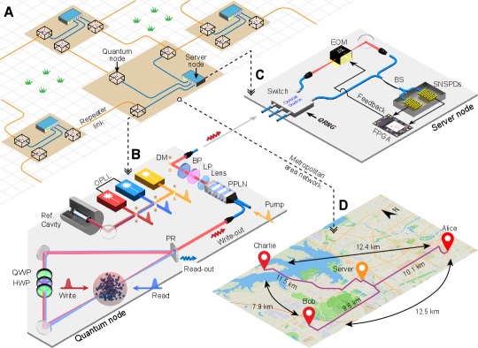
Quantum networks [1, 2] operate differently from their classical counterparts, as their nodes can store and process quantum information and are linked through the sharing of entangled states. The non-local nature of entanglement enables a range of disruptive applications such as quantum cryptography [3], distributed quantum computing [4], and enhanced sensing [5, 6]. Quantum nodes within a metropolitan area can be entangled through optical channels of a few tens of kilometers with a moderate transmission loss (e.g. dB for 50 km fiber at 1550 nm). For entangling intercity nodes, quantum repeater protocols [7, 8] need to be implemented to overcome the exponential growth in transmission loss. Fig. 1A envisions a wide area complex quantum network, consisting of a number of high-connectivity metropolitan area networks that are furthermore interconnected via quantum repeater channels.
The building block of a quantum network is the heralded entanglement between a pair of adjacent quantum nodes. This has been successfully demonstrated across various physical platforms including atomic ensembles [9, 10, 11], single atoms [12], diamond nitrogen-vacancy centers [13, 14, 15], trapped ions [16], rare-earth doped crystals [17, 18] and quantum dots [19, 20], among others. Currently, the maximum physical separation achieved is 1.3 km [14]. Building on this progress, three-node quantum network primitives have been established recently on a laboratory scale [21, 22, 23], opening up opportunities for multi-user applications such as the creation of three-body entangled GHZ states [21, 22], entanglement swapping between two elementary links [22], and qubit teleportation between non-neighboring nodes [23]. The next challenge is to extend these laboratory or short-scale experiments to a metropolitan scale, which needs the combination of several requirements: low fiber transmission loss, independent quantum nodes and a scalable network architecture. Thanks to the great progress of the quantum frequency conversion (QFC) technique [24], platforms operating at high transmission-loss wavelengths are now able to access the fiber network with minimal loss. This has enabled a series of works distributing local light-matter entanglement over up to a few kilometer fibers [25, 26, 27, 28, 29, 30]. Furthermore, two seminal experiments demonstrated heralded entanglement between two quantum nodes via long fiber links, one using two single atoms and 33 km of fiber [31] and the other using two atomic ensembles and 50 km of fiber [32]. However, the entanglement between two single atoms was generated at a low rate of approximately 1 min-1 and the entanglement between two atomic ensembles was generated between two non-independent nodes, raising concerns about their scalability towards large-scale and multi-user scenarios.
Here, we overcome these challenges with a set of key innovations and present a multinode quantum network over a metropolitan area. Our network consists of three quantum nodes (Alice, Bob, and Charlie) and a server node arranged in a star topology (Fig. 1D). The three quantum nodes are located on the three vertices of a triangle with sides of 7.9 km to 12.5 km in length in Hefei city, and run independently. The server node is situated approximately in the center of the triangle and linked to each quantum node via optical fibers for both classical and quantum communication. In each quantum node, a cavity enhanced laser-cooled Rubidium atomic ensemble serves as the long-lived quantum memory [33], generating atom-photon entanglement using the Duan-Lukin-Cirac-Zoller (DLCZ) protocol [34]. The photon is sent to the server node for entangling, while the atomic qubit is stored for subsequent applications. To reduce photon loss in the fiber, each quantum node is equipped with a QFC module, which coherently shifts visible photons at the Rubidium resonance to the telecom O band [32]. Quantum nodes are furthermore synchronized in phase using a remote phase stabilization method. Using this architecture, we demonstrated the generation of entanglement between distant quantum nodes and the storage of entanglement exceeding the round-trip communication time. Furthermore, we extended the remote entanglement generation to all three links in the network and executed them concurrently.
Network architecture for remote entanglement generation
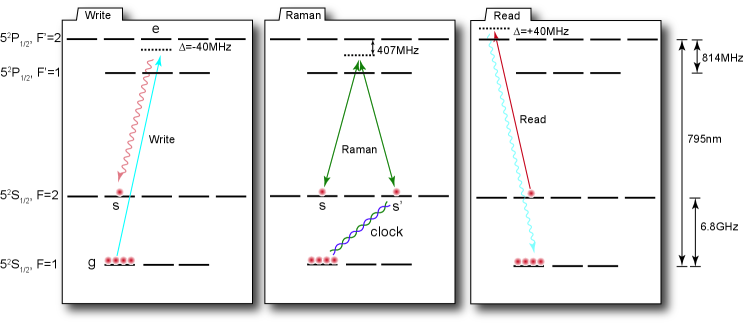
We generate remote entanglement between a pair of distant quantum nodes via a single photon scheme [34]. We start by preparing the light-matter entanglement in each quantum node (Fig. 1B) using the DLCZ protocol [34]. A weak write pulse induces a spontaneous Raman-scattered photon (write-out) in a small probability , whose presence and absence is associated to that of collective excitation of the atomic ensemble. This forms a Fock-basis light-matter entanglement , where and refer to the number of photon or atomic excitation, indicated by the subscript a and p, respectively, from hereafter. The atomic excitation can be stored up to 560 s until being retrieved for following operations [30]. The write-out photon is down-converted from 795 nm (3.5 dB/km) at Rubidium resonance to 1342 nm (0.3 dB/km) in the telecom O band in a periodically poled lithium niobate (PPLN) waveguide chip with the help of a strong 1950 nm Pump laser. The telecom photon then is sent to the server node for interference. The QFC module, including the down-conversion, noise filtering and fiber coupling, constitute an end-to-end efficiency of 46% and noise of Hz. In the server node (Fig. 1C), a beamsplitter combines the write-out photon from two quantum nodes and erases their which-path information. A click from a superconducting nanowire single photon detector (SNSPD) heralds the maximally entangled states between two ensembles
| (1) |
where the sign depends on the heralding detector. accounts for the optical phase difference accumulated during the entangling process, including and , the phase difference of Write lasers and of Pump lasers in two nodes, respectively, as well as , the phase difference of two fiber channels.
The key to the success of the single-photon scheme lies in accurately setting to a known value. To this end, previous laboratory experiments have typically used an ad hoc laser shared by separated nodes, and locked the closed-loop interferometer composed of the laser splitting paths and the quantum channels [9, 20, 32, 22, 17]. It adds complexity to the networking by requiring additional fiber and hardware resources and exposes the quantum nodes to the risk of potential attacks during quantum communication [35]. Crucially, additional unknown fiber phases are introduced to the generated state, which erases the state’s coherence.
To address these challenges, we developed a network architecture based on a weak-field remote phase stabilization method. The method relies on detecting the phase difference in situ at the entanglement generation facilities using weak-field phase probe (PP) pulses and photon counting, and compensating for it immediately, similar to that being realized recently in quantum key distribution experiments [36]. To obtain an accurate measurement of , we prepare a PP pulse with a length of s at the write-out photon’s frequency from the Read laser (due to its frequency likeness to the write-out photon) in each node, and use it to simulate the write-out photon’s transmission s earlier than the entanglement trial. Analogous to the entangling process, two PP pulses interfere in the server node, with the results reflected in the counts of SNSPDs. We extract the phase difference from the interference and compensate for it in an electro-optical modulator (EOM) before the interference beamsplitter. This method has three critical requirements for the PP pulses: their frequency difference is much smaller than , their linewidths are much narrower than and , and they inherit the same laser phase as the write-out photons. To meet these requirements, we lock all lasers in each node onto a reference cavity and get a linewidth of sub-kilohertz and a drift of a few kilohertz per day for all lasers. We perform a one-off frequency calibration of the corresponding lasers in different nodes. Additionally, we synchronize the Write and Read lasers using an optical phase-locked loop (OPLL). As a result, each PP pulse differs from the corresponding write-out photon with a phase , leading to a residual phase (the difference of in two nodes) in Eq. 1 after compensation. One can either remove by synchronizing the OPLLs in two nodes or choose as the phase reference to observe the entanglement. We chose the latter method in the following experiments.
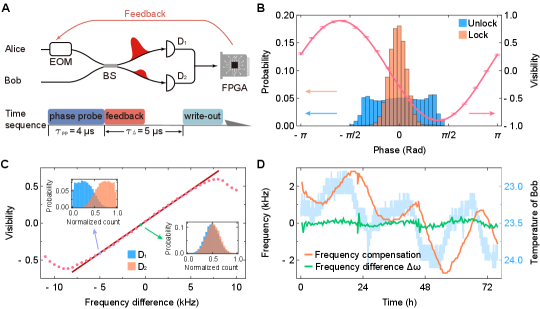
In practice, we conduct twice the phase stabilization in each trial for a better performance (Fig. 2A). To characterize the stabilization performance, we send an additional PP pulse from each quantum node 5 s after the feedback and find a Gaussian phase distribution with a standard deviation of 17∘, as shown in Fig. 2B. By changing the relative phase between the additional pair of PP pulses, we observe a sinusoidal oscillation of their interference visibility (Fig. 2B), which confirms a good phase correlation between two nodes.
An additional challenge in operations arises from the slow frequency drift of the reference cavities, which can transfer to the lasers and eventually to write-out photons. To avoid this, we employ a continuous frequency calibration using the PP interference data. We determine the minor laser frequency offset by analyzing the phase evolution between successive entanglement trials over a duration of and compensate it to the Pump lasers. Considering the long coherence time of the lasers ( ms) and the slow fluctuations in the fiber, the phase evolves solely due to . We verify this by observing the interference visibility as a function of shown in Fig. 2C. Through the implementation of the calibration, we are able to maintain kHz over a span of 76 hours, despite an observed drift of 5 kHz (Fig. 2D).
Entanglement between a pair of distant nodes
We first generate remote entanglement between Alice and Bob. In addition to laser frequency and phase stabilization, we apply polarization filtering using a fiber polarizing beamsplitter (PBS) for the photons when they arrive the server node and continuously adjust an electrical polarization controller before the PBS to maximize the filtering efficiency (not shown in the setup schematic). To measure the distant entanglement between the two atomic ensembles, we retrieve each atomic state to a photonic mode via a read pulse generated from the Read laser, and obtain . To evaluate the entanglement, one needs the knowledge of coherence between and . As it is experimentally hard to perform qubit operations in the Fock basis, prior experiments mostly inferred by interfering two read-out modes using a beamsplitter [9, 32, 17], which is not favorable for spatially separate cases. To overcome this challenge, we develop a method based on the weak-field homodyne measurement schemes [37, 38] that allows us to witness remote Fock-basis entanglement through local operations and measurements. Additionally, our method effectively converts the Fock-basis entanglement into a polarization maximally entangled (PME) state [34], making it accessible for entanglement-based communication schemes.
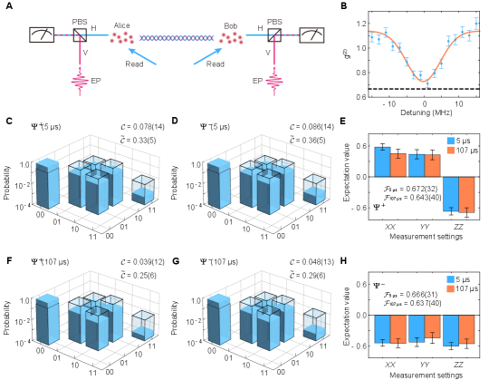
Our method starts by generating an entanglement probe (EP) pulse from the Write laser in each node. It is a weak coherent light field that has the same frequency and profile as the read-out field, but orthogonally polarized. When choosing the phase reference of , one can write the joint state of two EP pulses as , which is in phase with . Next, we combine the read-out field with the EP pulse in every node using a PBS and perform projection measurements under different polarization bases (Fig. 3A). Initially, we measure the mixed field in both nodes in the basis. On the detector corresponding to horizontal polarization, the EP is removed, thus we find , , , and through statistical analysis, where represents the probability of having excitations in Alice and excitations in Bob. When measuring in the superposition basis, the read-out field interfere with the EP pulses, resulting in remote correlation. Specifically, when basis is chosen, we have the correlation function
| (2) |
where represent the coincidence events between the mode in Alice and mode in Bob ( takes or , referring to and , respectively). In this case, we find . Now we can estimate the degree of entanglement with concurrence . This measure ranges from 0 for a separable state to 1 for a maximally entangled state.
Although being a good measure of entanglement, does not indicate how useful the entangled state is in entanglement-based communication. To answer this question, we consider the mixed field right after the combining PBS at each node, which can be approximated (with arbitrary phase factors and no normalization)
| (3) |
where is the identity operator and is the photon creation operator with the subscript indicating its node (Alice or Bob) and polarization ( or ). Selecting at least one photon at each node, Eq. 3 becomes
| (4) |
Neglecting the higher-order term , Eq. 4 is a PME state between two photonic modes. This allows local Pauli operations (, , and ) and enables entanglement based communication protocols. More details about the weak-field entanglement verification method are discussed in Ref. [39].
The weak-field method to verify remote entanglement relies on the EP pulse’s likeness to the read-out field. We examine this by performing a Hong-Ou-Mandel (HOM) experiment between these two fields. By scanning the detuning of the EP pulse, we observe a HOM dip in the correlation function shown in Fig. 3B, and get a minimum value of , close to the thermal-coherent interference limit of (the EP pulse is a coherent state and the read-out field without conditioning by the write-out field is a thermal state). This will lead to a 10% underestimation of in measurements [39].
Next, we verify the remote entanglement generated between Alice and Bob using the weak-field method. In the first experiment, we verify the entanglement in a delayed-choice fashion [40]. The atomic states are retrieved 5 s after the atom-photon entanglement is created, earlier than the entanglement is heralded. Fig. 3C and D summarize the reconstructed density matrices between the read-out fields and the corresponding . for both and witness the existence of remote entanglement. By deducting the loss during retrieval and detection, we infer the density matrices between two atomic ensembles and their corresponding concurrence to two atomic ensembles and show them in the same figures. Meanwhile, we find the fidelity for and 0.666(31) for to corresponding maximally entangled state, both above 0.5 to certify the entanglement (Fig. 3E and H). In the second experiment, we create the remote entanglement in the same fashion but store it for s, exceeding the round-trip transmission time between the quantum and the server nodes. We get a slightly lower concurrence result for each case, as summarized in Fig. 3F and G. However, the fidelities of are on par with that of the former experiment (Fig. 3E and H). Comparing the variation of and between two experiments, we confirm that a large portion of noise in the generated entangled states is the vacuum component and can be effectively filtered out using our weak-field method and other protocols [34]. The measured heralding probability is and for the first and second experiments, respectively, which corresponds to an entangling rate of 1.93 Hz and 0.83 Hz, considering the experiment repetition rate of 2.76 kHz and 1.03 kHz.
Concurrent entanglement generation in the network
| Alice-Bob | Alice-Charlie | Bob-Charlie | ||
|---|---|---|---|---|
| 0.086(14) | 0.074(14) | 0.032(12) | ||
| 0.086(14) | 0.063(13) | 0.048(13) | ||
| 0.38(5) | 0.35(5) | 0.17(5) | ||
| 0.38(5) | 0.30(5) | 0.23(5) |
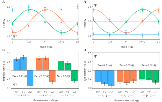
Now we complete the network architecture by including the third quantum node, Charlie, and concurrently generate entanglement , and on three links, Alice-Bob, Bob-Charlie and Alice-Charlie, respectively. To this end, the server node is equipped with a multi-input-two-output optical switch and assigns two of the three users to the detection upon request. In our demonstration, we assign a 5.8 s time slot for each pair of users and dynamically switch user pairs according to a quantum random number generator (QRNG), simulating unknown requests in real-world applications. Since different links are frequently switched, a ‘hot swapping’ feature is crucial, i.e. the entangling conditions are meet immediately after switching. In our architecture, the phase stabilization is executed for every entanglement trial and is unaffected by switching. The good laser stability guarantees ignorable relative frequency drift although a 1/3 effective calibration time is assigned for each pair of nodes. Furthermore, we store the optimal EPC parameters for the polarization filtering to each specific fiber and load them during switching.
We first observe the local manipulation of non-local states. For instance, when applying a unitary operation locally at one of the quantum nodes (e.g., Charlie), its relevant non-local states ( and ) change in form while the entanglement is preserved. The irrelevant non-local states remain unchanged. In practice, we vary the phase at Charlie and measure the correlation of each pair of entanglement. As shown in Fig. 4A and B, we observe sinusoidal oscillations in the expected pairs and , while contributes a constant in this measurement. A delay between the oscillations of and arises from the phase stabilization mechanism [39].
In the end, we characterize the generated remote entangled states on three links in the delayed-choice fashion. Tab. 1 summarizes the concurrence results and and Fig. 4C, D show the correlation measurement results of the PME states. For all three links, we find to confirm the presence of atomic entanglement and to witness the entanglement in corresponding PME state. The entangled states between Alice and Bob are comparable to that generated in the fixed connection case, indicating no extra decoherence being introduced in the switching process. The lower entanglement quality in other links arises from experimental imperfections [39]. The entangling rates of all three links are roughly 1/3 of that measured in the fixed connection case as expected. Some simple upgrades to the server node will immediately improve the networking performance, such as parallel (rather than concurrent) creation of multiple entanglement pairs with the help of wavelength division multiplexing technique [41] and genuine three-body entanglement creation using a modified interferometer [42, 21, 43].
Discussion and outlook
In this work, we present the debut implementation of a metropolitan area entanglement-based quantum network. With this facility, we have successfully demonstrated the heralded generation of remote entanglement between two quantum nodes separated by 12.5 km and store it longer than the two-way communication time. We also showed the concurrent generation of multiple entanglement pairs within the network. The high entangling rate in our network is enabled by a series of methods, two of which are crucial. Firstly, the remote phase stabilization guarantees the basis to implement the single photon scheme. In addition, it provides a flexible and scalable network infrastructure that can accommodate more quantum nodes within the metropolitan area. Secondly, the weak-field method simplifies the verification of remote Fock-basis entanglement. It removes the necessity to interfere two remote Fock-basis photons, instead only requires local linear optics operations and measurements. Moreover, using this method, one can effectively convert Fock-basis entanglement to polarization maximally entanglement, making entanglement-based communication within the reach. Adapting these methods to other physical platforms will accelerate their networking process.
Further advances of the network performance will happen in four main aspects, increasing the entangling rate by shifting the wavelength to telecom C band [27, 31] and by adapting multiplexed atomic quantum memories [44, 45, 46]; decreasing the entanglement infidelity by suppressing unwanted higher order atomic excitations with the help of Rydberg blockade mechanism [38, 47]; realizing a better entanglement verification by filtering out the vacuum components in the remote entangled state [34, 10] or by using nonlinear atomic state detection techniques [48, 49]; and prolonging the entanglement storage time to the second scale by further limiting atomic thermal motion with optical lattice technique [50, 51]. With these improvements, we expect remote entanglement can be generated much faster than it is lost, laying the basis for mediating serval metropolitan area quantum networks via quantum repeater protocols [7, 8].
Acknowledgment
We acknowledge QuantumCTek for the allocation of node Bob, and Hefei Institutes of Physical Science for the allocation of node Charlie. Funding: This research was supported by the Innovation Program for Quantum Science and Technology (No. 2021ZD0301104), National Key R&D Program of China (No. 2020YFA0309804), Anhui Initiative in Quantum Information Technologies, National Natural Science Foundation of China, and the Chinese Academy of Sciences. Competing interests: The authors declare no competing interests. Data and materials: The data are archived at Zenodo [52].
References
- Kimble [2008] H. J. Kimble, Nature 453, 1023 (2008).
- Wehner et al. [2018] S. Wehner, D. Elkouss, and R. Hanson, Science 362, eaam9288 (2018).
- Gisin et al. [2002] N. Gisin, G. Ribordy, W. Tittel, and H. Zbinden, Reviews of Modern Physics 74, 145 (2002).
- Jiang et al. [2007] L. Jiang, J. M. Taylor, A. S. Sørensen, and M. D. Lukin, Physical Review A 76, 062323 (2007).
- Gottesman et al. [2012] D. Gottesman, T. Jennewein, and S. Croke, Physical Review Letters 109, 070503 (2012).
- Kómár et al. [2014] P. Kómár, E. M. Kessler, M. Bishof, L. Jiang, A. S. Sørensen, J. Ye, and M. D. Lukin, Nature Physics 10, 582 (2014).
- Briegel et al. [1998] H.-J. Briegel, W. Dür, J. I. Cirac, and P. Zoller, Physical Review Letters 81, 5932 (1998).
- Sangouard et al. [2011] N. Sangouard, C. Simon, H. de Riedmatten, and N. Gisin, Reviews of Modern Physics 83, 33 (2011).
- Chou et al. [2005] C. W. Chou, H. de Riedmatten, D. Felinto, S. V. Polyakov, S. J. van Enk, and H. J. Kimble, Nature 438, 828 (2005).
- Chou et al. [2007] C.-W. Chou, J. Laurat, H. Deng, K. S. Choi, H. de Riedmatten, D. Felinto, and H. J. Kimble, Science 316, 1316 (2007).
- Yuan et al. [2008] Z.-S. Yuan, Y.-A. Chen, B. Zhao, S. Chen, J. Schmiedmayer, and J.-W. Pan, Nature 454, 1098 (2008).
- Hofmann et al. [2012] J. Hofmann, M. Krug, N. Ortegel, L. Gérard, M. Weber, W. Rosenfeld, and H. Weinfurter, Science 337, 72 (2012).
- Bernien et al. [2013] H. Bernien, B. Hensen, W. Pfaff, G. Koolstra, M. S. Blok, L. Robledo, T. H. Taminiau, M. Markham, D. J. Twitchen, L. Childress, and R. Hanson, Nature 497, 86 (2013).
- Hensen et al. [2015] B. Hensen, H. Bernien, A. E. Dréau, A. Reiserer, N. Kalb, M. S. Blok, J. Ruitenberg, R. F. L. Vermeulen, R. N. Schouten, C. Abellán, W. Amaya, V. Pruneri, M. W. Mitchell, M. Markham, D. J. Twitchen, D. Elkouss, S. Wehner, T. H. Taminiau, and R. Hanson, Nature 526, 682 (2015).
- Humphreys et al. [2018] P. C. Humphreys, N. Kalb, J. P. J. Morits, R. N. Schouten, R. F. L. Vermeulen, D. J. Twitchen, M. Markham, and R. Hanson, Nature 558, 268 (2018).
- Moehring et al. [2007] D. L. Moehring, P. Maunz, S. Olmschenk, K. C. Younge, D. N. Matsukevich, L.-M. Duan, and C. Monroe, Nature 449, 68 (2007).
- Lago-Rivera et al. [2021] D. Lago-Rivera, S. Grandi, J. V. Rakonjac, A. Seri, and H. de Riedmatten, Nature 594, 37 (2021).
- Liu et al. [2021] X. Liu, J. Hu, Z.-F. Li, X. Li, P.-Y. Li, P.-J. Liang, Z.-Q. Zhou, C.-F. Li, and G.-C. Guo, Nature 594, 41 (2021).
- Delteil et al. [2016] A. Delteil, Z. Sun, W.-B. Gao, E. Togan, S. Faelt, and A. Imamoğlu, Nature Physics 12, 218 (2016).
- Stockill et al. [2017] R. Stockill, M. J. Stanley, L. Huthmacher, E. Clarke, M. Hugues, A. J. Miller, C. Matthiesen, C. Le Gall, and M. Atatüre, Physical Review Letters 119, 010503 (2017).
- Jing et al. [2019] B. Jing, X.-J. Wang, Y. Yu, P.-F. Sun, Y. Jiang, S.-J. Yang, W.-H. Jiang, X.-Y. Luo, J. Zhang, X. Jiang, X.-H. Bao, and J.-W. Pan, Nature Photonics 13, 210 (2019).
- Pompili et al. [2021] M. Pompili, S. L. N. Hermans, S. Baier, H. K. C. Beukers, P. C. Humphreys, R. N. Schouten, R. F. L. Vermeulen, M. J. Tiggelman, L. d. S. Martins, B. Dirkse, S. Wehner, and R. Hanson, Science 372, 259 (2021).
- Hermans et al. [2022] S. L. N. Hermans, M. Pompili, H. K. C. Beukers, S. Baier, J. Borregaard, and R. Hanson, Nature 605, 663 (2022).
- Kumar [1990] P. Kumar, Optics Letters 15, 1476 (1990).
- De Greve et al. [2012] K. De Greve, L. Yu, P. L. McMahon, J. S. Pelc, C. M. Natarajan, N. Y. Kim, E. Abe, S. Maier, C. Schneider, M. Kamp, S. Höfling, R. H. Hadfield, A. Forchel, M. M. Fejer, and Y. Yamamoto, Nature 491, 421 (2012).
- Bock et al. [2018] M. Bock, P. Eich, S. Kucera, M. Kreis, A. Lenhard, C. Becher, and J. Eschner, Nature Communications 9, 1998 (2018).
- van Leent et al. [2020] T. van Leent, M. Bock, R. Garthoff, K. Redeker, W. Zhang, T. Bauer, W. Rosenfeld, C. Becher, and H. Weinfurter, Physical Review Letters 124, 010510 (2020).
- Tchebotareva et al. [2019] A. Tchebotareva, S. L. N. Hermans, P. C. Humphreys, D. Voigt, P. J. Harmsma, L. K. Cheng, A. L. Verlaan, N. Dijkhuizen, W. de Jong, A. Dréau, and R. Hanson, Physical Review Letters 123, 063601 (2019).
- Krutyanskiy et al. [2019] V. Krutyanskiy, M. Meraner, J. Schupp, V. Krcmarsky, H. Hainzer, and B. P. Lanyon, npj Quantum Information 5, 72 (2019).
- Luo et al. [2022] X.-Y. Luo, Y. Yu, J.-L. Liu, M.-Y. Zheng, C.-Y. Wang, B. Wang, J. Li, X. Jiang, X.-P. Xie, Q. Zhang, X.-H. Bao, and J.-W. Pan, Physical Review Letters 129, 050503 (2022).
- van Leent et al. [2022] T. van Leent, M. Bock, F. Fertig, R. Garthoff, S. Eppelt, Y. Zhou, P. Malik, M. Seubert, T. Bauer, W. Rosenfeld, W. Zhang, C. Becher, and H. Weinfurter, Nature 607, 1 (2022).
- Yu et al. [2020] Y. Yu, F. Ma, X.-Y. Luo, B. Jing, P.-F. Sun, R.-Z. Fang, C.-W. Yang, H. Liu, M.-Y. Zheng, X.-P. Xie, W.-J. Zhang, L.-X. You, Z. Wang, T.-Y. Chen, Q. Zhang, X.-H. Bao, and J.-W. Pan, Nature 578, 240 (2020).
- Bao et al. [2012] X.-H. Bao, A. Reingruber, P. Dietrich, J. Rui, A. Dück, T. Strassel, L. Li, N.-L. Liu, B. Zhao, and J.-W. Pan, Nature Physics 8, 517 (2012).
- Duan et al. [2001] L.-M. Duan, M. D. Lukin, J. I. Cirac, and P. Zoller, Nature 414, 413 (2001).
- Pang et al. [2020] X.-L. Pang, A.-L. Yang, C.-N. Zhang, J.-P. Dou, H. Li, J. Gao, and X.-M. Jin, Physical Review Applied 13, 034008 (2020).
- Zhou et al. [2023] L. Zhou, J. Lin, Y. Jing, and Z. Yuan, Nature Communications 14, 928 (2023).
- Tan et al. [1991] S. M. Tan, D. F. Walls, and M. J. Collett, Physical Review Letters 66, 252 (1991).
- Li et al. [2013] L. Li, Y. O. Dudin, and A. Kuzmich, Nature 498, 466 (2013).
- [39] Materials and methods are available as supplementary materials.
- Ma et al. [2012] X.-S. Ma, S. Zotter, J. Kofler, R. Ursin, T. Jennewein, Č. Brukner, and A. Zeilinger, Nature Physics 8, 479 (2012).
- Wengerowsky et al. [2018] S. Wengerowsky, S. K. Joshi, F. Steinlechner, H. Hübel, and R. Ursin, Nature 564, 225 (2018).
- Choi et al. [2010] K. S. Choi, A. Goban, S. B. Papp, S. J. van Enk, and H. J. Kimble, Nature 468, 412 (2010).
- Dür et al. [2000] W. Dür, G. Vidal, and J. I. Cirac, Physical Review A 62, 062314 (2000).
- Collins et al. [2007] O. A. Collins, S. D. Jenkins, A. Kuzmich, and T. A. B. Kennedy, Physical Review Letters 98, 060502 (2007).
- Pu et al. [2017] Y.-F. Pu, N. Jiang, W. Chang, H.-X. Yang, C. Li, and L.-M. Duan, Nature Communications 8, 15359 (2017).
- Parniak et al. [2017] M. Parniak, M. Dąbrowski, M. Mazelanik, A. Leszczyński, M. Lipka, and W. Wasilewski, Nature Communications 8, 2140 (2017).
- Sun et al. [2022] P.-F. Sun, Y. Yu, Z.-Y. An, J. Li, C.-W. Yang, X.-H. Bao, and J.-W. Pan, Physical Review Letters 128, 060502 (2022).
- Xu et al. [2021] W. Xu, A. V. Venkatramani, S. H. Cantú, T. Šumarac, V. Klüsener, M. D. Lukin, and V. Vuletić, Physical Review Letters 127, 050501 (2021).
- Yang et al. [2022] C.-W. Yang, C.-W. Yang, C.-W. Yang, J. Li, J. Li, J. Li, M.-T. Zhou, M.-T. Zhou, M.-T. Zhou, X. Jiang, X. Jiang, X. Jiang, X.-H. Bao, X.-H. Bao, X.-H. Bao, X.-H. Bao, J.-W. Pan, J.-W. Pan, J.-W. Pan, and J.-W. Pan, Optica 9, 853 (2022).
- Yang et al. [2016] S.-J. Yang, X.-J. Wang, X.-H. Bao, and J.-W. Pan, Nature Photonics 10, 381 (2016).
- Wang et al. [2021] X.-J. Wang, S.-J. Yang, P.-F. Sun, B. Jing, J. Li, M.-T. Zhou, X.-H. Bao, and J.-W. Pan, Physical Review Letters 126, 090501 (2021).
- [52] J.-L. Liu, X.-Y. Luo, Y. Yu, C.-Y. Wang, B. Wang, Y. Hu, J. Li, M.-Y. Zheng, B. Yao, Z. Yan, D. Teng, J.-W. Jiang, X.-B. Liu, X.-P. Xie, J. Zhang, Q.-H. Mao, X. Jiang, Q. Zhang, X.-H. Bao, and J.-W. Pan, Data for "A multinode quantum network over a metropolitan area", zenodo (2023); https://doi.org/10.5281/zenodo.8149009.
SUPPLEMENTAL MATERIAL
I Details of the experimental setup
I.1 General details
We cool down and trap the atomic ensemble using a magneto-optical trap (MOT). We run the MOT at a repetition rate of Hz. In each MOT cycle, we cool down the atoms in the first 25 ms/24 ms (for a storage time of 5 s/107 s), pump the atoms to the specific Zeeman ground state in the next 1 ms, and perform the entanglement measurement using the rest time. Each entanglement trial takes 33 s in the delayed-choice measurements and 131 s when storing the qubit longer than the round-trip communication time, leading to an average experimental repetition rate of 2.76 kHz and 1.03 kHz.
Fig. S1 depicts the energy level scheme of three main steps at each quantum node, i.e., the write, read process of the DLCZ quantum memory and the spin-wave freezing technique using the Raman operations. More details of the energy level and the spin-wave freezing technique are discussed in Ref. [1].
I.2 Experimental control and synchronization
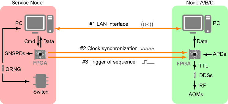
Fig. S2 depicts the schematic of our experimental control system. In each network node, a field programmable gate array (FPGA) takes charge of time sequence generation and data acquisition. The acquiesced data are instantaneously uploaded to a computer for storage. The FPGA in the server node disseminates its clock signal and experimental triggers to the quantum nodes via optical fibers for experiment synchronization. In the server node, we store the random number taken from the quantum random number generator [2] for data synchronization. More details of the system control and synchronization can be found in our previous paper [1].
II The phase of entanglement states
Here we give a complete description of the phase involved in the remote entanglement generation and verification. Fig. S3 depicts a detailed schematic of a quantum node. The notations used in the following derivation and their corresponding description are listed in Tab. S1.
| Notations | Description |
|---|---|
| The time for the write-in or read-out operation, respectively. | |
| The initial phase of the Write laser at time . | |
| The initial phase of the Pump laser at time . | |
| The initial phase of the Read laser at time . | |
| The optical path phase of the Write pulse. | |
| The optical path phase of the Read pulse. | |
| The part of accumulated in the local interferometer. | |
| The part of accumulated outside the local interferometer. | |
| The optical path phase of the write-out photon. | |
| The part of accumulated in the local interferometer. | |
| The part of accumulated outside the local interferometer. | |
| The optical path phase of the read-out photon. | |
| The optical path phase of the EP pulse. | |
| The phase accumulated during atomic storage. | |
| The total phase of the write-out-read-out photon pair. | |
| The feedback phase of the EOM at the server node. | |
| The local phase related to a single node. | |
| The remote phase related to two nodes. | |
| The phase of the PME state. |
We start from the local atom-photon entanglement pair generation. The interference and the detection of the write-out photons herald the entanglement of two atomic ensembles. Then the atomic excitations are retried as photons for entanglement verification. The retrieval and write-out photon detection processes are communitive, so we consider a delayed-choice experiment where the atomic state is retrieved immediately after its creation. In this case, the local entanglement between the write-out and the read-out photon mode reads
| (S1) |
where
| (S2) |
correspond to the phase of the fiber channel in the main text. With a click event of an SNSPD, the remote entangled state reads
| (S3) |
Apart from the phase of photon pairs , the phase is involved because the phase feedback is applied before the remote entanglement generation.
During the entanglement verification, we combine an EP pulse with the read-out photons at each node. We generate the EP pulse from the Write laser (because of its frequency likeliness with the read-out photon). Hence the EP pulse inherits the initial phase of the Write laser. In the limit of weak power, we can write the joint state of two EP pulses in two nodes as follows,
| (S4) |
We encode the read-out photon modes in Eq. S3 in the horizontal polarization (), the EP pulse mode in Eq. S4 in the vertical polarization mode () and combine them using PBSs (shown in the Fig. 3A of the main text). By selecting one photon at each node, we obtain a polarization maximally entangled (PME) state
| (S5) |
We define as the phase of the PME state,
| (S6) |
where we divide the total phase into the local phase at nodes A and B () and the remote phase between two nodes (). They are given by:
| (S7) |
| (S8) |
In the expression of (Eq. S7), the first term stands for the phase during the storage in the atomic ensembles. The first bracket represents the phase difference of some optical paths, constituting an interferometer highlighted in Fig. S3. The second bracket indicates the phase inherited from the lasers at different times.
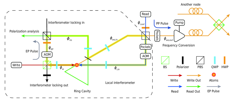
To keep stable in the 100 s time scale, we reduce the Zeeman energy level fluctuation of atoms by securing a constant magnetic environment (see Ref. [1]) and transferring the spin wave to clock transition to reduce the sensitivity to the magnetic field. The stable laser phase is guaranteed by locking lasers to a stable and narrow linewidth reference cavity. To stabilize the local interferometer, we inject a locking beam during the MOT loading phase and apply the feedback onto a mirror glued with a piezo-electric transducer. The acousto-optic modulators (AOMs) on the optical paths function as frequency shifters. One shifts the PP pulse to the write-out photon’s frequency during the phase probing phase, and the other shifts the EP pulse to the read-out photon’s frequency during the entanglement verification phase.
We lock the remote phase with the weak-field remote phase stabilization methods. For practical reasons, we add an addition in the feedback (i.e. ), which implies,
| (S9) |
By adding three equations in Eq. S9, we get:
| (S10) |
which explains the phase delay between and in Fig. 4A and 4B in the main text.
III The model of entanglement verification
Using the EP pulses, we can transfer the Fock state entanglement to PME states, which makes entanglement verification much simpler. Thus, we can use entanglement fidelity to quantify the quality of entanglement. Here, we give the form of entanglement fidelity and show the limitation under our experimental imperfections.
III.1 The model of the state and the measurement
The click of an SNSPD heralds the entanglement of two atomic ensembles. We consider the atomic state being retrieved as read-out photons. The density matrix of the joint read-out state under the Fock basis reads [3]
| (S11) |
where represents photons at Alice and photons at Bob, and represents the coherence term. To certify the remote entanglement, we generate an EP pulse at each quantum node, which is essentially a weak coherent pulse resembling the read-out mode in all degree-of-freedoms. The density matrix of the joint EP state is
| (S12) |
where () represents the phase of the EP pulses at Alice (Bob). We encode the read-out photon onto the horizontal polarization, the EP pulse onto the vertical polarization and mix them using a PBS at each node. The state after mixing reads
| (S13) |
After mixing, we perform the polarization projection measurement. We register the events where only one detector clicks at each node. When measuring at the basis, the four associated observables reads
| (S14) |
where represents the detection of a photon with polarization at node A and a photon with polarization at node B with ( takes or ).
III.2 PME states and their fidelity estimation
We define the state in Eq. S13 when choosing one photon at each node as a polarization maximally entangled (PME) state. The correlator of the PME state can be calculated as
| (S15) |
Similarly, the correlator can be calculated as,
| (S16) |
The observables represent the detection of a photon with polarization at node A and a photon with polarization at node B. We get them using the basis transformation
| (S17) |
where is the mode mixing operator. The correlator has the same form as , so we omit it here.
By fixing the phase of the EP pulses, we target the PME states to two Bell state , with the sign depending on the phase of the initial atomic entanglement. We can estimate the fidelity of the PME states to their target Bell state as
| (S18) |
Substituting the expressions of the correlators we learn that the fidelity is a function of the EP state intensity . In our experiments, we set to maximize the fidelity. After ignoring the higher-order terms, , the fidelity is given by:
| (S19) |
where and . The former describes the coherence between and , which can also be understood as the interference visibility when we combine two read-out modes with a beamsplitter, and the latter describes the contribution of high order excitations.
To have more insight of the PME fidelity, we associate the fidelity expression with the atomic state. We define as atomic excitations at node A and at node B upon an SNSPD heralding the remote entanglement between two atomic ensembles. We can associate and using the retrieval efficiency ,
| (S20) |
where we neglected the small contribution from on . The non-zero part of comes from the incorrect heralding of the SNSPD, such as a dark count. is given by the higher-order atomic excitations. We estimate them as follows,
| (S21) |
where SNR is the signal-to-noise ratio of write-out photon, and is the internal excitation probability. Then we can get:
| (S22) |
Substituting it into Eq. S19, we obtain:
| (S23) |
From the above equation, retrieval efficiency does not significantly affect fidelity, while internal excitation probability and SNR play a significant role.
III.3 Concurrence
Concurrence is a widely used entanglement criterion for Fock state entanglement. Due to its monotonicity under local operation and classical communication (LOCC), for the read-out photons verifies the entanglement of the atomic ensembles at two nodes. The key to estimating the entanglement is the coherence term measurement, which is usually done by interfering with the read-out photons and measuring the visibility [3, 4, 5]. Here, we show that we can give a lower bound on according to the visibility in the basis, and thus we can give a lower bound on the concurrence.
From Eq. S16, we can get:
| (S24) |
Then, we can get:
| (S25) |
where is the absolute value of the correlator XX/YY. Then, the concurrence is given by:
| (S26) |
According to the data measured in basis, we can get the photon statistics of the read-out photons. Furthermore, with (we use the mean value of and to calculate ) we can give a lower bound on the concurrence .
III.4 Photon transmission losses and non-unit detection efficiency
The above calculations are based on unit detection efficiency, and the losses during the photon transmission are not considered. This section will show that these two factors do not affect the above conclusion.The non-unit transmission efficiency of a mode can be modeled by a BS with transmission of , whose operator is:
| (S27) |
where is the mode we care about, and is an auxiliary mode that models the losses of photons in mode. This loss operator, on the one hand, describes the losses due to all kinds of optical devices; on the other hand, it describes the non-unit detection efficiency. The partial density matrix of the total density matrix S12 at one node is a mixture of general two-mode quantum state, which is given by:
| (S28) |
where is the Fock state basis. The general two-mode quantum state can be also transferred to the coherent state basis with the completeness relation:
| (S29) |
Then, it can be written in the form:
| (S30) |
In coherent state basis, it’s easy to check the following equation:
| (S31) |
which means that after tracing all the auxiliary modes , we can exchange the position of the loss operator and the mode mixing operator . So, in the basis the non-unit detection efficiency is equivalent to the losses before the mode mixing operation. This equivalence in the basis is trivial.
Now, we can concentrate on the losses of EP pulses and the read-out photons. For the former one, we can get:
| (S32) |
which shows that losses only change the amplitude of the EP pulses. For the latter, the losses can be regarded as a decrease in the retrieval efficiency, which does not change the form of the density matrix S11. Thus, by adjusting the amplitude of the EP pulses and redefining the density matrix of the read-out photons(including all the losses and the limited detection efficiency), the conclusion derived in the ideal cases still works in the realistic experimental parameters.
IV Data analysis
IV.1 The imperfection of
We have given the form of the visibility in basis in Eq. S16. We find that it is subject to the following inequality:
| (S33) |
where the equality holds under the condition , which is approximately satisfied in our experiments. Then we can compare the experimental results with , where can be given by definition or estimated from the experimental parameters according to Eq. S22. The results are given in Tab. S2:
| Storage time (ST) | ||||
| Storage time (ST) | ||||
| A-B | ||||
| A-C | ||||
| B-C | ||||
We can see that the experimental results agree well with the estimated value .
IV.2 The imperfection of
In Eq. S24, we have shown that the visibility is bounded by . The parameter captures the imperfection due to the high-order excitations, and the left part , defined as , describes the coherence of the Fock state entanglement. It can also be interpreted as the interference visibility of the read-out photons when two read-modes are combined with a BS. Here, we focus on several experimental imperfections that reduce the visibility , and we use to represent the maximum visibility under a particular factor.
IV.2.1 High order excitations
The photon counts distribution contain the contribution of high order excitations, which reduce the interference visibility. Considering the balanced retrieval efficiency and the atomic excitation distribution , the photon count distribution can be given by:
| (S34) |
where the high order excitation terms are estimated as . The maximum visibility is given by:
| (S35) |
With the mean retrieval efficiency and the internal excitation probability substituted into the above equation, we get the maximum visibility , as shown in Tab. S3:
IV.2.2 The indistinguishability of the read-out photons and the EP pulses
We use Hong-Ou-Mandel (HOM) interference to estimate the indistinguishability of the read-out photons and the EP pulses. The unnormalized density matrix of the read-out photons and the phase-randomized EP pulses can be given by:
| (S36) |
where are the average photon numbers of read-out photons and the EP pulses, represent the probability of two-photon term, and higher order terms are ignored. In ideal cases, of the read-out photons is given by 2, and of the EP pulses is given by 1. After mixing two fields with a BS, we can get the coincidence probability:
| (S37) |
The first and second terms come from the two-photon component in the read-out photons and EP pulses, and the last term comes from the single-photon component of both fields. If they are completely indistinguishable, the last term disappears, and represents the indistinguishability of two fields [6]. When both fields are on, is given by:
| (S38) |
When , reaches its minimum value of . We get by setting , and then measuring . The measurement results of three nodes are listed in Tab. S4.
The indistinguishability of the read-out photons and the EP pulses will affect the visibility . We use the following polarization entangled state to model this imperfection:
| (S39) |
where is the other degree of freedom of photons,, represent the indistinguishability parameter at two nodes. In the superposition basis, the visibility is given by . This value describes the decrease of due to the mode mismatch, and related experimental results are given in Tab. S5
IV.2.3 The imbalance between and
The imbalance of and , which stems from the imbalance of the internal excitation probability , the transmission efficiency of write-out photons and the retrieval efficiency , will also lead to the decrease of . We have given the density matrix of the read-out photons in Eq. S11. The positive semidefiniteness of the density matrix puts an upper bound on :
| (S40) |
With the definition of , we get:
| (S41) |
The above equation shows the limitation of due to the imbalance of , and the experimental results are given in Tab. S6:
We can see that the imbalance of decreases the visibility little.
IV.2.4 The phase instability
The phase instability is the critical factor that reduces the visibility . The polarization entanglement states with a phase uncertainty can be written as: . Considering a distribution of , the average visibility is given by:
| (S42) |
We assume that follows a Gaussian probability distribution with a mean of 0 and a standard deviation () of . Then, we will get:
| (S43) |
which shows that the of the phase is the critical parameter we need to consider.
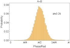
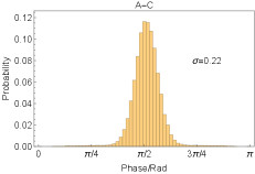
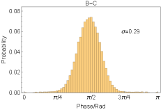
In the part , we have given the phase of the entanglement states in connection: . Then the is given by two local phases and one remote phase . We estimate the of the remote phase with the photon distribution of the phase probe laser after phase locking. The results are given in Fig. S4. Due to the higher phase noise of the lasers in node B, the phase locking performance in the A-B/B-C connection is worse than in the A-C connection.
As for the local phase , it consists of three parts: the memory phase , the interferometer phase and the laser phase . The memory phase is determined by the magnetic field at the atoms and the storage time:
| (S44) |
The fluctuation of the magnetic field, which has a characteristic frequency of 50 Hz, is mainly caused by the surrounding power supplies. The SD of the magnetic field in three nodes is given by . With the storage time of about , we can get the SD of the memory phase, as shown in Tab. S7. As for the extended storage time experiments, the spin wave is transferred to clock transition, leading to three orders of magnitude reduction of the magnetic field sensitivity so that we can neglect the extra memory phase fluctuation due to longer storage time.
The phase instability coming from the local interferometers is estimated according to the interference signal after the phase locking, and the locking performance is also shown in Tab. S7. The significant difference in interferometer locking precision is due to vibration noise in the environment.
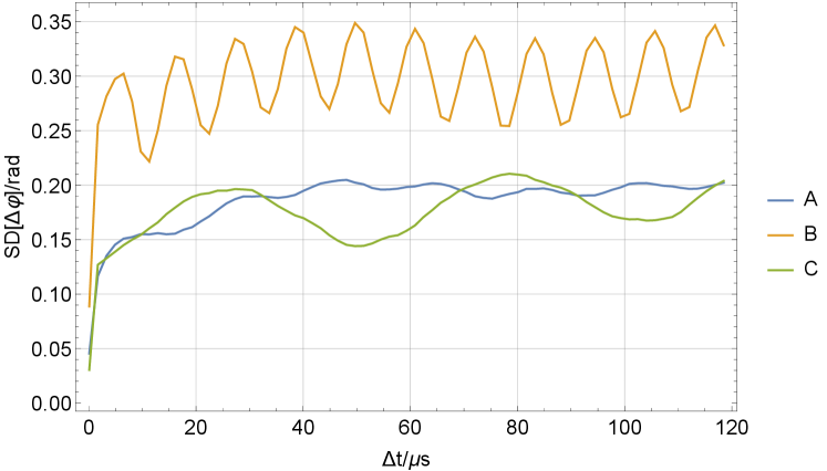
The last part of the phase instability comes from the lasers. We estimate according to the beat frequency of the write and read lasers, which are locked to an ultra-stable cavity and then phase-locked to each other. The beat signal at 6.8GHz is shifted to the DC range with a microwave signal source and a frequency mixer, and then recorded with an oscilloscope, whose bandwidth is 500 MHz. In this way, we can measure the phase difference of write and read laser: , and then we can estimate the phase instability of lasers by , where , is the storage time. The measurement results are given in Fig. S5 and Tab. S7. The phase oscillation shows the characteristic frequency noise of the lasers at each node.
| Standard Deviation/rad | node | node | node |
|---|---|---|---|
| 0.084 | 0.035 | 0.018 | |
| 0.029 | 0.135 | 0.063 | |
| 0.14 | 0.31 | 0.14 | |
| 0.20 | 0.33 | 0.17 |
With all the phase instability given above, the total of the local phase is given by:
| (S45) |
Then the phase instability of the entanglement state of two nodes A and B is estimated as:
| (S46) |
From Eq. S43 , we can evaluate the influence of the total phase instability on the visibility, and the results are given in Tab. S8
| 0.89 | 0.88 | 0.89 | 0.95 | 0.89 |
IV.2.5 Summary
| High order excitations | |||||
|---|---|---|---|---|---|
| Mode mismatch | |||||
| Phase instability | 0.89 | 0.88 | 0.89 | 0.95 | 0.89 |
| Imbalance of Read-out photons | |||||
In the above sections, we have discussed several experimental imperfections that reduce the visibility :
1. The high order excitations.
2. The indistinguishability of the read-out photons and the EP pulses.
3. The imbalance between and .
4. The phase instability.
The main reducing factors are the high-order excitations, the mode mismatch, and the phase instability. At the same time, the imbalance of the read-out photons has little influence. For different quantum nodes, the laser phase noises at node B are much larger than the other two. Due to more considerable transmission losses of the field deployed optical fibers between node C and the server node, we set a little higher internal excitation probability at node C to balance the transmission losses. These two factors result in worse visibility in the B-C connection. Here, all the maximum visibility under these experimental imperfections are summarized in Tab. S9, and we multiply them together as to estimate their total contribution. The experimental results , calculated according to its definition, are also given in Tab. S9. The experimental results are lower than the theoretical estimate, which hints other uncaptured experimental imperfections. For example, the slow laser intensity drift of the local interferometer locking beam will lead to the drift of the phase locking point, thus reducing the visibility .
References
- [1] X.-Y. Luo, et al., Physical Review Letters 129, 50503 (2022).
- [2] Y.-Q. Nie, et al., Review of Scientific Instruments 86, 063105 (2015).
- [3] C. W. Chou, et al., Nature 438, 828 (2005).
- [4] Y. Yu, et al., Nature 578, 240 (2020).
- [5] D. Lago-Rivera, S. Grandi, J. V. Rakonjac, A. Seri, H. de Riedmatten, Nature 594, 37 (2021).
- [6] L. Li, Y. Dudin, A. Kuzmich, Nature 498, 466 (2013).