A Nearly Similar Powerful Test for Mediation
Abstract
This paper derives a new powerful test for mediation that is easy to use.
Testing for mediation is empirically very important in psychology,
sociology, medicine, economics and business, generating over 100,000
citations to a single key paper. The no-mediation hypothesis also poses a theoretically interesting statistical
problem since it defines a manifold that is non-regular in the origin where
rejection probabilities of standard tests are extremely low. We prove that a
similar test for mediation only exists if the size is the reciprocal of an
integer. It is unique, but has objectionable properties. We propose a new
test that is nearly similar with power close to the envelope without these
abject properties and is easy to use in practice. Construction uses the
general varying -method that we propose. We illustrate the results in an
educational setting with gender role beliefs and in a trade union sentiment
application.
Keywords: Varying -method, Mediation, Indirect Effect, Power Envelope, Similar Tests, Invariant Tests, Optimal Tests
Version October, 2021
1 Introduction
This paper derives a new powerful test for mediation that is easy to use. Testing for mediation effects is empirically extremely important in various scientific disciplines. A key paper in psychology, Baron and Kenny (1986) has more than 100,000 citations111 Cited by 106,782 on 13 October 2021, 90,147 on 15 January 2020, and 79,205 on 22 October 2018. and is used in many other fields. Mediation testing is important in accounting, e.g. Coletti et al. (2005), marketing, e.g. MacKenzie et al. (1986), sociology, e.g. Alwin and Hauser (1975) who used the expression indirect effect, a term commonly used in economics also.For a recent overview of mediation in economics see Huber (2020) and e.g. Heckman and Pinto (2015a, b) on treatment effects and production technology, and Imbens (2020) who extensively reviews connections between directed acyclic graphs (DAGs), potential outcomes, causal inference, instrumental variables, and mediation. Frewen et al. (2013) is exemplary for the increasing network literature, including DAGs, using mediation. The minimal selection here is hardly representative for the vast body of literature on mediation analysis. It only illustrates the breadth of its empirical relevance. Tests for mediation can have extremely low power, especially when the effect is small, or estimated with large variance. The primary purpose of this paper is to provide a new and more powerful test that is easy to use.
The aim of mediation testing is to discover if an independent variable () causes a dependent variable () via an intervening, or mediating variable (). The mediating variable is exogenous in the common experimental setting in psychology and other fields, but is also considered exogenous in other settings where assignments are random or constitute a natural experiment. The basic model is simply:
| (1) | ||||
| (2) |
where all variables are taken in deviation from their means, or more generally after partialing out other exogenous effects. The disturbances and are assumed to be independent because of an experimental set up and more generally because no influence of on is assumed in this type of model. This independence is a crucial identification condition, since the parameter cannot be estimated consistently if is endogenous. We make a convenient distributional assumption: , with the number of observations. This facilitates a likelihood analysis, but is not necessary for the asymptotic normality of the -statistics that will be used.
MacKinnon et al. (2002) give a literature review and compare 14 different methods for testing the effects of a mediation variable. These methods are based on standardized measures of the product of two coefficients or based on the difference of two related coefficients () in equations (1) and (3):
| (3) |
If there is a mediation effect, then influences such that and influences such that If there is no mediation by then the effect of on is not altered by the inclusion of such that
Model (3) is a restricted version of (1) with and it is straightforward therefore to show that the OLS estimates for the three models satisfy and the relation also holds in model interpretation terms; see Appendix A.

Figure 1 illustrates mediation, no mediation, and the related concept of moderation in terms of directed acyclic graphs. is a moderator if it changes the relation between and . In its basic form this is modeled by adding the interaction term between and to the model. When confounders are observed and included we have:
| (4) |
can also be included in (1) - (3), but partialed out such that , and are residuals after regressions on Moderation and confoundedness can be tested by the ordinary or tests on and but testing for mediation is less straightforward.
The best well known and commonly used test for mediation by Sobel (1982) is a Wald-type test of the form , with an estimate of the standard error of the product It is available in standard statistical packages such as SAS, R, Stata, or SPSS. It has good properties when either or is large and the standard errors of and are small, but if the two -tests for testing and tend to be small, properties deteriorate. For parameter values under the null, the Null Rejection Probability (NRP) can be very close to zero and, under the alternative, power can fall far below the size (highest NRP) of that we use throughout. All tests considered in MacKinnon et al. (2002) suffer from these problems. The distributions of the test statistics considered in the literature depend on the value of the parameters under the null. As a consequence none of these tests is similar, meaning that rejection probabilities are not constant on the boundary of the null hypothesis. In fact rejection probabilities under alternatives close to the origin, i.e. power, can be much lower than size and these tests are biased.
Much effort in the literature has gone into improving well-known test statistics, such as the Wald statistic, without a satisfactory solution. The bootstrap is invalid (see Van Garderen and Van Giersbergen (2021)) and cannot salvage these statistics. The key step in our approach is to move away from test statistics and consider the critical region in the sample space directly and optimize the flexible boundary we define.
We make two main contributions. Our main theoretical contribution in Theorem 2 shows that a similar mediation test exists if and only if the level of the test is the reciprocal of an integer, i.e. or . Hence, for practical levels such as , or an exact similar test exists. The proof is constructive and the test is unique within the class considered. Unfortunately, the critical region is objectionable in that it includes an area near the origin where both -statistics are arbitrarily close to zero. Such values do not provide overwhelming evidence against the null and Perlman and Wu (1999) coined the term “Emperor’s New Tests” for similar tests with undesirable properties like these. Insistence on similarity can render LR tests -inadmissible, cf. Lehmann and Romano (2005, Section 6.7), but Perlman and Wu (1999) give examples where similar tests have extremely undesirable properties, yet inadmissible LR tests still provide reasonable answers. In the mediation setting the LR test is also inadmissible, but does not provide a satisfactory answer in this case. It is much better than the Wald test as we will see, but nevertheless suffers from extremely poor power properties for parameter values close to the origin.
So a better test is called for and our second, more important contribution therefore is practical. We construct a new simple test for mediation that is uniformly more powerful than the LR test without the undesirable properties sketched by Perlman and Wu (1999), and that is nearly similar and practically unbiased.
It is extremely simple to use:
- 1.
- 2.
| 0 | 0.01 | 0.02 | 0.03 | 0.04 | 0.05 | 0.06 | 0.07 | 0.08 | 0.09 | |
|---|---|---|---|---|---|---|---|---|---|---|
| 0.0 | 0 | 0.01 | 0.02 | 0.03 | 0.04 | 0.05 | 0.06 | 0.07 | 0.08 | 0.09 |
| 0.1 | 0.1 | 0.10672 | 0.10672 | 0.10672 | 0.10672 | 0.10672 | 0.11672 | 0.12671 | 0.13670 | 0.14669 |
| 0.2 | 0.15669 | 0.16668 | 0.17667 | 0.18666 | 0.19666 | 0.20665 | 0.21664 | 0.22663 | 0.23663 | 0.24662 |
| 0.3 | 0.25661 | 0.26660 | 0.27660 | 0.28659 | 0.29658 | 0.30658 | 0.31657 | 0.32656 | 0.33655 | 0.34655 |
| 0.4 | 0.35654 | 0.36653 | 0.37652 | 0.38652 | 0.39651 | 0.40650 | 0.41649 | 0.42649 | 0.43648 | 0.44647 |
| 0.5 | 0.45646 | 0.46646 | 0.47645 | 0.48644 | 0.49643 | 0.50643 | 0.51642 | 0.52641 | 0.53640 | 0.54640 |
| 0.6 | 0.55639 | 0.56638 | 0.57637 | 0.58637 | 0.59636 | 0.60635 | 0.61634 | 0.62634 | 0.63633 | 0.64632 |
| 0.7 | 0.65631 | 0.66631 | 0.67630 | 0.68629 | 0.69628 | 0.70628 | 0.71627 | 0.72626 | 0.73625 | 0.74625 |
| 0.8 | 0.75624 | 0.76623 | 0.77622 | 0.78622 | 0.79621 | 0.80620 | 0.81620 | 0.82619 | 0.83618 | 0.84617 |
| 0.9 | 0.85617 | 0.86616 | 0.87615 | 0.88614 | 0.89614 | 0.90613 | 0.91612 | 0.92611 | 0.93611 | 0.94610 |
| 1.0 | 0.95609 | 0.96608 | 0.97608 | 0.98607 | 0.99606 | 1.00605 | 1.01605 | 1.02604 | 1.03603 | 1.04602 |
| 1.1 | 1.05602 | 1.06601 | 1.07600 | 1.08599 | 1.09599 | 1.10598 | 1.11597 | 1.12596 | 1.13596 | 1.14595 |
| 1.2 | 1.15594 | 1.16593 | 1.17593 | 1.18592 | 1.19591 | 1.20590 | 1.21590 | 1.22589 | 1.23588 | 1.24587 |
| 1.3 | 1.25587 | 1.26586 | 1.27585 | 1.28584 | 1.29584 | 1.30583 | 1.31286 | 1.31310 | 1.31310 | 1.31310 |
| 1.4 | 1.31310 | 1.31310 | 1.31310 | 1.31310 | 1.31310 | 1.31750 | 1.32750 | 1.33750 | 1.34750 | 1.35750 |
| 1.5 | 1.36750 | 1.37750 | 1.38750 | 1.39750 | 1.40750 | 1.41750 | 1.42750 | 1.43750 | 1.44750 | 1.45750 |
| 1.6 | 1.46750 | 1.47750 | 1.48750 | 1.49750 | 1.50750 | 1.51750 | 1.52750 | 1.53750 | 1.54750 | 1.55750 |
| 1.7 | 1.56750 | 1.57750 | 1.58750 | 1.59750 | 1.60750 | 1.61750 | 1.62750 | 1.63750 | 1.64750 | 1.65750 |
| 1.8 | 1.66750 | 1.67750 | 1.68750 | 1.69750 | 1.70750 | 1.71750 | 1.72750 | 1.73750 | 1.74750 | 1.75750 |
| 1.9 | 1.76750 | 1.77750 | 1.78750 | 1.79750 | 1.80750 | 1.81750 | 1.82750 | 1.83750 | 1.84750 | 1.85750 |
| 2.0 | 1.86750 | 1.87750 | 1.88750 | 1.89750 | 1.90750 | 1.91750 | 1.92750 | 1.93750 | 1.94750 | 1.95750 |
| 2.1 | 1.95996 | 1.95996 | 1.95996 | 1.95996 | 1.95996 | 1.95996 | 1.95996 | 1.95996 | 1.95996 | 1.95996 |
That the test can be based on elementary -statistics is important for ease of application, but is theoretically justified below by sufficiency and invariance arguments. The testing problem is invariant to permutations of parameters and statistics and sign changes. We show that the ordered absolute -statistic, is a maximal invariant. The critical region is a subset of the relevant sample space which is an octant in . This can also be justified asymptotically under very weak assumptions and different estimation methods.
The new test is constructed by varying the boundary of the critical region, defined as a function , such that the test is almost similar and minimizing the distance to the power envelope surface. It is based on a new general, so called varying- method that can be applied to other testing problems with nuisance parameters more generally to obtain near similar tests. It does not require a choice of mixture distribution, nor the construction of least favorable distributions, cf. Andrews and Ploberger (1994), Andrews et al. (2006, 2008), Elliott et al. (2015), Guggenberger et al. (2019). It can be given a random critical value interpretation as in Moreira and Mourão (2016) since any critical region in a higher-dimensional space has a boundary for one statistic in terms of the remaining statistics. The critical region that we construct is fixed however, not random, avoids simulation, and our approach appears to lend itself better to multivariate extensions, as will be shown for dimension three.
We use and develop numerical methods that avoid simulations and use numerical integration instead. With the required computing completed for the mediation problem, practitioners can simply use Table 1 or the computer code provided in the appendix. In fact no further reading on the motivation and derivation of the test is required for its implementation.
Section 5 shows the ease of implementation using an interesting application by Alan et al. (2018) on educational attainment. The test confirms that the negative effect on girls’ attainment of 1-year exposure to teachers with traditional attitudes, is mediated through students’ own gender role beliefs. Neither the procedure in Alan et al. (2018) nor the LR test reject the no mediation hypothesis in this case, but our new test does.
A further empirical illustration on union sentiment among southern nonunion textile workers is provided in Section 7. Different mediation channels are tested involving two mediating variables and requires an extension of our methods. We therefore consider general hypotheses of the form . We give the relevant distributions of maximal invariants that can be used to derive the critical regions that are nearly similar and do so explicitly for three dimensions.
For practitioners the major advantage of our test is that there is a better chance of formally showing that there is a mediation effect. Our test has better power, especially when the two channeling effects are small or less accurately estimated. Given the enormous interest in testing for mediation and the fact that our test can have close to more power than standard level tests, many unpublished examples will exist where it can now be concluded that there is a statistically significant mediation effect.
2 Theory
The joint density of given in equations (1) and (2) can be written as:
with , , and . The parameters , and vary freely as a result of the triangular structure of the model. The mediation variable is the endogenous variable in (2), but is exogenous for in (1) since is not causal for . For a sample of independent observations the loglikelihood equals the sum of two normal loglikelihoods corresponding to (1) and (2)222This can easily be extended to include more regressors/covariates. Instrumental variables can also be used, but note that and appear in both equations and in the standard setup and are independent because of the experimental interpretation of . All that is required is the asymptotic normality of the estimators and -statistics.:
| (5) |
As a consequence the Maximum Likelihood Estimators (MLEs) for and are the basic OLS estimators for the two equations separately. Furthermore, both observed and expected Fisher information matrices will be block diagonal in terms of and as well as in , , and As a result the standard -statistics and for and respectively are asymptotically independent and normally distributed with means , where , denote the true parameter values and , the standard deviations of the OLS estimators: , with
Restricting attention to can be justified by statistical sufficiency, since the MLE is minimal sufficient and complete, and by invariance since the values of and do not affect whether is true or not. Hillier et al. (2021) show that is a maximal invariant under a relevant group of transformations. The testing problem has two more obvious symmetries. The problem is not affected by sign changes or permutations. This also holds in higher dimensions, e.g. when mediation is through a chain of effects as in our empirical illustration. If then parameters are required to be non-zero for this channel to operate. In dimensions the null hypothesis that at least one parameter is zero and the alternative is all parameters non-zero:
There are many other hypotheses including collapsibility in contingency tables, testing indirect effects, channels in DAGs, see Dufour et al. (2017) for a range of examples.
In the multivariate setting we also assume that the estimator is normally distributed with known covariance matrix . Hence, if we let and such that are the -ratios and are the non-centrality parameters, we assume:
Assumption 1
:
The testing problem is invariant to reordering the parameters (permutations) and sign changes (reflections) of the parameters . The group of permutations, say, has elements and the group of sign changes, say, has elements (two possible signs for each element). The groups and have only the identity element in common, but are otherwise non-overlapping. The full group generated by and therefore has elements. Exploiting the invariance and symmetry properties of the problem reduces the domain of integration by a factor . This is important because all optimizations require probabilities calculated by numerical integration. The density after a sign change in is obtained by a corresponding sign change in and for a permutation of also permutes accordingly. Hence for any element we have or so the distribution is invariant; see Lehmann and Romano (2005).
Theorem 1
The testing problem is invariant under the group of transformations acting on and , given Assumption 1. The absolute order statistic with is a maximal invariant statistic and the absolute order parameter with is a maximal invariant parameter under the group of transformations The distribution of depends only on
The Wald and LR tests are functions of the maximal invariant and so will our new test. The density is required for probability calculations and optimizations for the new test. It is easily derived for arbitrary dimension using Equation (6) of Vaughan and Venables (1972):
Lemma 1
The probability density function of the absolute order statistic is given by:
| (6) |
with the permanent333The permanent is defined as with the sum over all permutations of the numbers akin the determinant but without the signature of the permutation. of the square matrix and the noncentral Chi-distribution with one degree of freedom and noncentrality parameter .
The noncentral Chi-distribution with one degree of freedom equals the folded normal distribution and if then the density of can be written as for . Substitution in Lemma 1 and simplifying gives the following result that is the basis for the numerical calculations that follow:
Lemma 2
The density of the ordered absolute -statistics for the mediation hypothesis is:
The ordered squared -statistic could also be used as maximal invariant. Lemma 1 would then lead to a density in terms of noncentral Chi-squared distributions.
2.1 Problems with Standard (Single) Mediation Test Statistics
Standard mediation test statistics used in practice have distributions that depend on the parameter values under the null. The rejection probabilities are therefore not constant and the tests are biased with power dropping below the size of the test, especially in a neighborhood of the origin. We illustrate the issue for the classic Wald and LR tests.
The null hypothesis defines a manifold that is almost everywhere continuously differentiable, with the exception of the origin which is a so-called “double point” where the two restrictions and , each defining a one-dimensional line, coincide. The widely used Sobel (1982) test equals the square root of the Wald test. Glonek (1993) derives the asymptotic distribution for the Wald test statistic:
| (7) |
As a consequence the asymptotic critical value for when both and is but jumps to i.e. the usual Chi-squared critical value for one restriction, for any other value. The discrete jump in the asymptotic distribution from the origin to any other fixed parameter is remarkable and shows explicitly that the distribution depends heavily on the parameter values under the null. This discontinuity in the asymptotic distribution and dependence on the parameter also invalidates bootstrap procedures and they are oversized. For an NRP of at the origin the critical value should be but this would lead to over-rejection for other values under the null and the test would be oversized (size ) and invalid. One could consider drifting sequences of parameter values to investigate the behavior of the Wald statistic near the origin, but that would not solve the problem. The problematic behavior of the Wald test under the null with singularities is well documented by Drton and Xiao (2016) and Drton (2009). No satisfactory solution has been found in the preceding decades to salvage the Wald statistic, see e.g. Dufour et al. (2017). This prompted our investigation and to propose an alternative solution.
The LR test was shown by Van Giersbergen (2014) to equal:
| (8) |
and rejects when both and are rejected by basic -tests. In MacKinnon et al. (2002) this is referred to as the test for joint significance, but not identified as the LR test. The rejection probability for critical value is:
by independence of and . These rejection probabilities are monotonically increasing in the absolute values of and . Correct size is therefore obtained by choosing the critical value of the test by letting when or if to guarantee that the rejection probability under the null is always smaller than or equal to the nominal size. The asymptotic critical value is therefore the usual . The NRP will depend on the values of and and vary between the following two extremes:
where is the upper percentile of the standard normal distribution. For an NRP of at the origin the critical value should equal . This leads to massive over-rejection if only one parameter is zero and the other much larger. The test with this critical value is oversized size and invalid.
The third classic test, the Lagrange Multiplier (LM) or score test, is even more problematic because its definition depends on parameter values under the null and there are three different versions depending on which , or both ’s are zero.
All these classic tests are functions of two -statistics. Their distributions, as well as their NRPs, clearly depend on the parameter values under the null and the tests are not similar. A test is called similar on the boundary of if the probability of rejecting the null is constant for all parameter values on the boundary of and . For mediation, this boundary equals itself and consists of the horizontal and vertical axes of the space. None of the classic tests is similar and in a neighborhood of the origin the NRPs are close to zero. As a result the power in a neighborhood of the origin is also close to zero and far below the size of the test and the tests are biased since there are parameter values with probability of rejection under the alternative lower than under the null.
2.2 Critical Regions
The behavior and construction of the classic test statistics is problematic. Given that no satisfactory adjustments of classic test statistics have been found, despite considerable efforts over recent decades, a different approach is required.
In order to derive an alternative test procedure we shift the focus from the test statistic to the critical region (CR). A critical region defines a test statistic of course, but choosing a class of tests, such as Wald, LR, or LM tests, restricts the shape of the critical region. For the same reason the tests focusing on improving the standard error of or analyzed in MacKinnon et al. (2002) restrict possible shapes of the critial region.
We construct a new test procedure by constructing the critical region directly by determining its shape in the two-dimensional sample space of the -statistics used in the construction of the tests. We consider critical regions that are bounded by a function and reject when We impose some weak regularity conditions. In particular we assume that is a càdlàg function from (including 0) to This will allow to have jumps, but limits the number of jumps to countably many. We also insist that is weakly increasing. This assures that a rejection (acceptance) for a realization is not reversed when either or is increased (decreased). This reasoning also motivates a CR that is (topologically) simply connected. Denote the set of weakly increasing càdlàg functions by , as in the common Skorokhod space notation, but here with weak monotonicity.
Definition 1
A function is called the boundary function (of the critical region) when it defines:
| Critical Region | |||
| Acceptance Region |
Justification for only using -statistics is by sufficiency and invariance. First, the MLE is a complete minimal sufficient statistic. The model constitutes a full exponential model since the dimensions of the minimal sufficient statistic and the parameter space are equal; see Van Garderen (1997). Second, and have distributions under the null that are independent of the nuisance parameters and Hillier et al. (2021) shows that, also in finite samples, is a maximal invariant under an appropriate group of transformations generalizing the scale invariance of the -statistics. Theorem 1 shows that as a consequence of the permutation and reflection invariance only of the two-dimensional sample space of needs to be considered and we define the critical region in the first octant (east to north-east). The other seven octants in follow by symmetry. The test defined by is indeed invariant to permutations, reflections, and scale transformations. The domain of can therefore be restricted to the non-negative real line and bounded by the line:
We can put the definition of a similar test in terms of the boundary function , noting that is itself the boundary of and :
Definition 2
is said to be a similar boundary function if the probability of the critical region defined by is constant under :
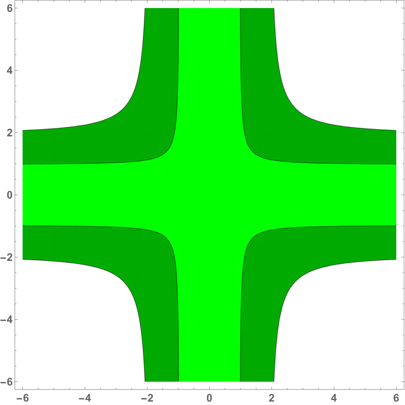
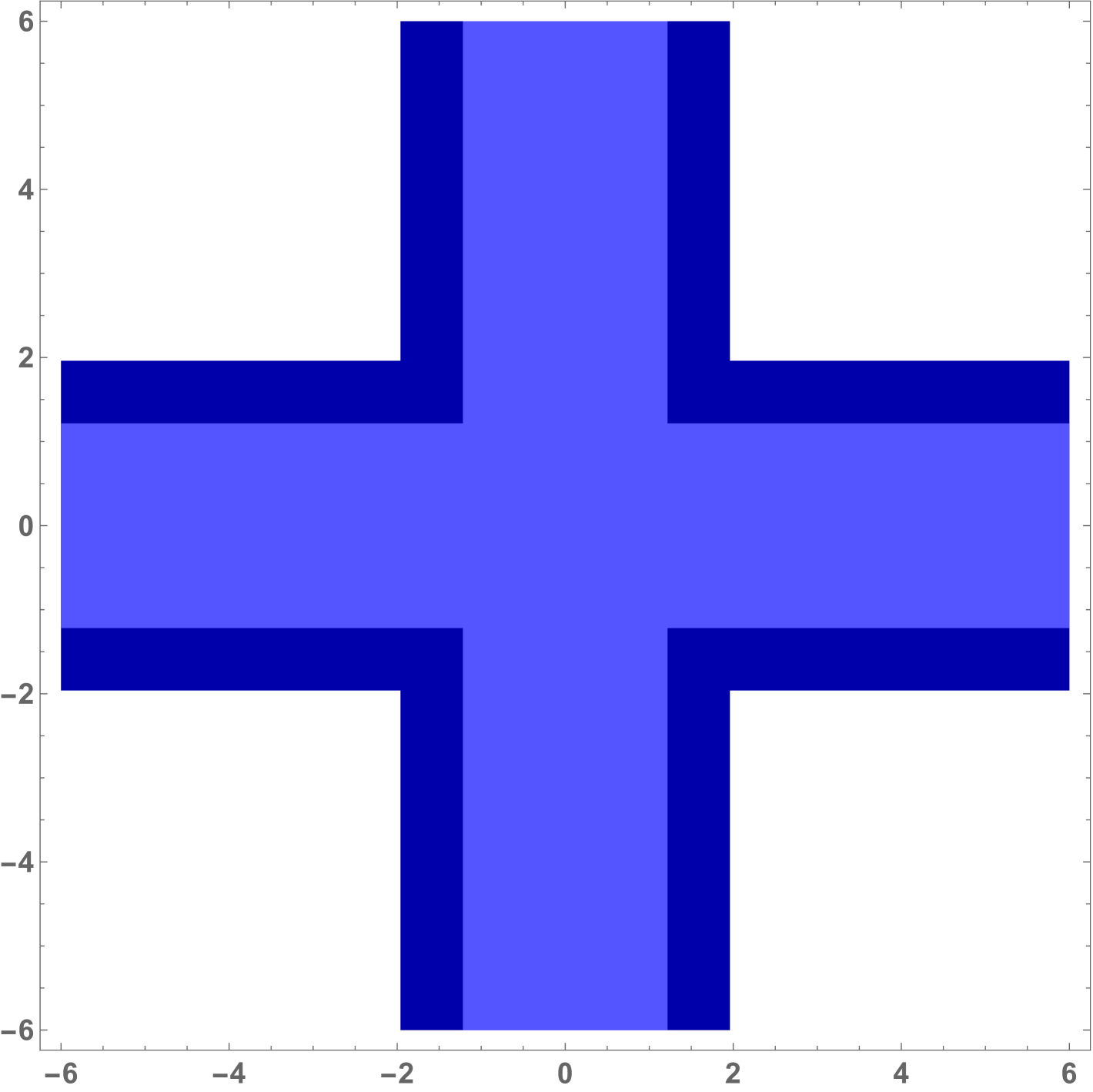
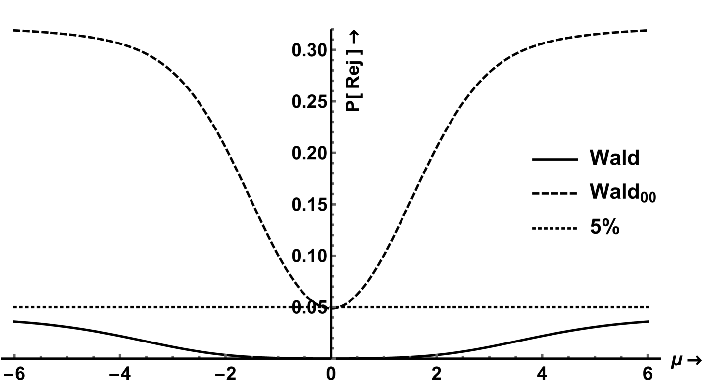
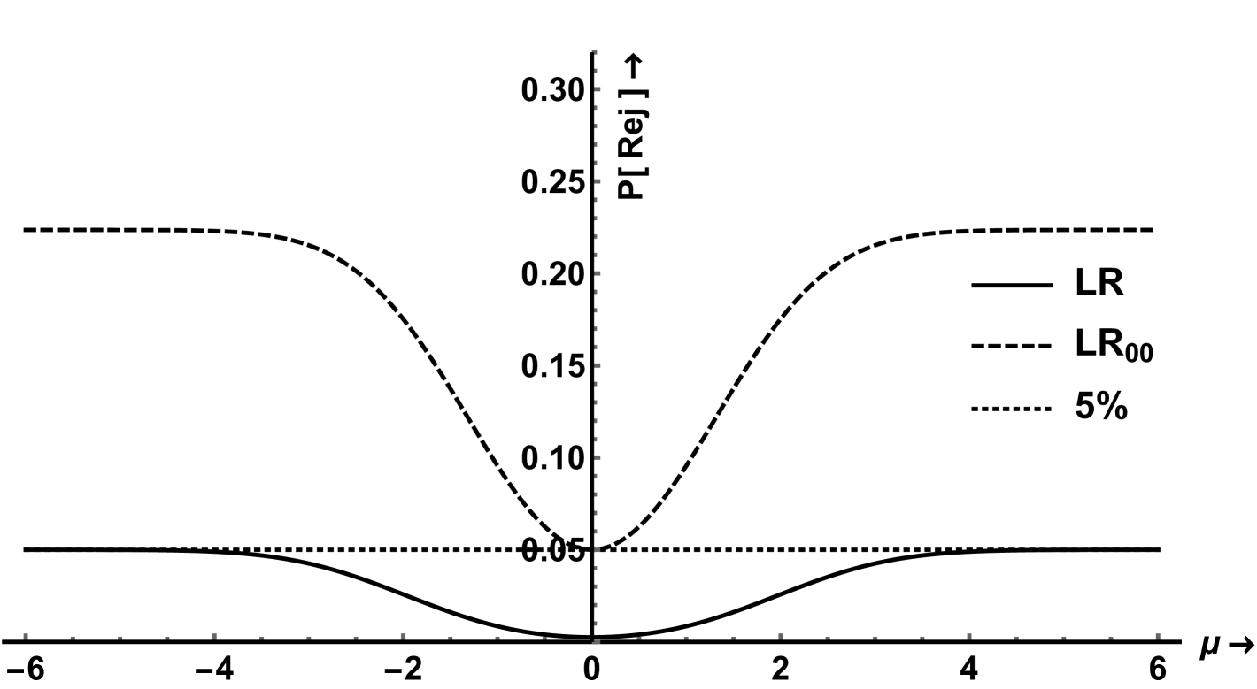
The boundary functions defined by the Wald (Sobel) and LR are not similar. Figures 2(a) and 2(b) show the boundary functions that define the critical region in terms of for the Wald and LR test. We show the boundaries for two critical values: one such that for large or the NRP is asymptotically. This value is the usual for the Wald test and for the LR test. The second, smaller critical value is such that the NRP is when This value is for the Wald test and for the LR test. The rejection probabilities are shown as a function of the noncentrality parameter for given such that holds. For the LR test with critical value the NRP goes down to when In the second case, with the smaller critical value , the NRP is by construction when but this is not a valid test since for other values the NRPs are much higher than the nominal size of . The same situation will occur when constructing point optimal invariant tests. The Wald test is considerably worse than the LR test with lower NRP over a wider range of , see figures 2(c) and 2(d).
The trinity of classic tests is clearly nonsimilar. The question is if we can do much better. Does there exist a similar test or is this a problem that is intrinsically unsolvable? The next theorem, and the main theoretical contribution, answers this question.
Theorem 2
A similar boundary function exists for testing if and only if is an integer (or trivially ). If it exists, the boundary is unique in
For common significance levels, including , , and , the theorem proves that exact similar tests exist. The proof is given in Appendix C and exploits the symmetries of the problem and the completeness of the normal distribution. The proof is constructive showing that the function must be a step function and is unique within the class of weakly increasing càdlàg functions. For the exact similar boundary is shown in Figure 3.
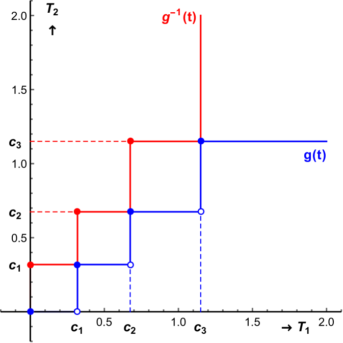
The CR shows a clear parallel with Figure 2 of Berger (1989). The step function starts horizontal and defines a CR with objectionable features. In particular, the CR will include all such that . For this corresponds to rejection when both -statistics are smaller than in absolute value (but non-zero) (for and smaller than and respectively). Such -statistics close to zero cannot be characterized as strong evidence against the null, in favor of both and being non-zero. Nevertheless, the test is size correct and renders the LR test -inadmissible. So it is an “Emperor’s New Tests” in the terminology of Perlman and Wu (1999) and does not provide a satisfactory solution to the problem of finding a better test. A second unattractive feature of this exact similar boundary is that for increasing values of the test statistics parallel and close to the diagonal, the decision alternates between rejection and acceptance, despite the fact that evidence against the null appears monotonically increasing.
Given the uniqueness of the similar test, we relax the strict similarity requirement and consider a class of near similar tests with NRPs that differ from by no more than . Within this class of so called -similar tests given in Definition 3 below, we determine a test that avoids the objectionable properties of the exact similar test, but achieves good power properties. Within this class of near similar tests we determine the power envelope and determine the test that minimizes the distance between its power surface and this power envelope. This new test is therefore optimal in this sense. It is easy to implement using Table 1 or using the R-code in Appendix E.
The first step in the composition of this optimal test is a new general method for constructing near similar tests.
3 Near Similar Test Construction: Varying g-Method
A general method for constructing near similar tests involves three generic steps:
-
1.
Define a flexible boundary for the critical region in the relevant sample space.
-
2.
Define a criterion function that penalizes the deviation of the NRP from the level for a grid of parameter values under the null (and possibly restrictions on and other aspects deemed relevant).
-
3.
Systematically vary and determine such that it minimizes the criterion function and is therefore as close to similarity as possible in the metric defined by .
The relevant sample space is determined by the particular testing problem at hand and may have been reduced by sufficiency, invariance, or other principles, to dimension , say. The boundary of the critical and acceptance region is then of dimension , but may consist of disjoint parts if the critical and/or acceptance region are not simply connected in a topological sense. There are various possibilities to define flexibly, but we will use splines.
The criterion function may include aspects other than similarity, for instance smoothness and monotonicity of , convexity of the critical or acceptance regions, or even rejection probabilities under alternatives. Consequently, Step 3 will generally be a constraint optimization problem. The systematic variation of is intended to be in line with the optimization routine used to minimize as in, e.g. a Newton-Raphson-type procedure.
For mediation testing with an exact test exists, but the varying -method may not find it because (i) is not flexible enough (ii) includes criteria other than NRPs (iii) numerical difficulties determining the jumps (iv) and finally restrictions to purposely exclude objectionable CRs.
An explicit implementation of the varying -method to the mediation problem is given next.
3.1 Near Similar Mediation g-Test
Step 1 in the varying -method is to determine the relevant sample space for the testing problem. The first dimensional reduction is to the MLE which is minimal sufficient and complete. The second reduction to follows from location-scale type invariance shown in Hillier et al. (2021). Permutation and reflection symmetries further reduce the relevant sample space to one octant according to Theorem 1. The maximal invariant is the ordered absolute -statistic with density given in Lemma 2 . For general , the rejection probability (RP) for the -method is given by:
| (9) |
This two-dimensional integral can be reduced to a one-dimensional integral by expressing the inner integral in terms of the CDF of the standard normal distribution :
| (10) | |||||
The RP thus simplifies to a one-dimensional integral by integrating formula (10) for over , which greatly improves efficiency and accuracy.
All NRPs in the paper were determined by numerical integration over under the null with . The numerical integration was performed in Julia, see Bezanson et al. (2017), using the function quadgk that is based on adaptive Gauss-Kronrod quadrature. For the final -function, the estimated upper bound on the absolute error for the calculated NRP is approximately .
The -boundary is generally determined by an algorithm and Appendix D shows the basic implementation of the varying -method using linear splines with knots, with the first and last knots fixed. In spite of its simplicity, it leads to big improvements even for small values of . Figure 4 illustrates the construction of the -function for a fixed number of grid points and the resulting in the sample space of , the East to North-East octant of .
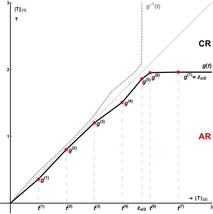
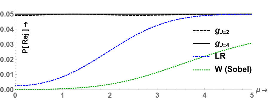
Figure 5 shows the NRPs of the test in comparison to the LR and Wald (Sobel) tests. There is a remarkable gain in the lowest NRP, and therefore local power, from to . Already for there is a large improvement and after gains are small, and beyond there was hardly any improvement.
3.2 Power
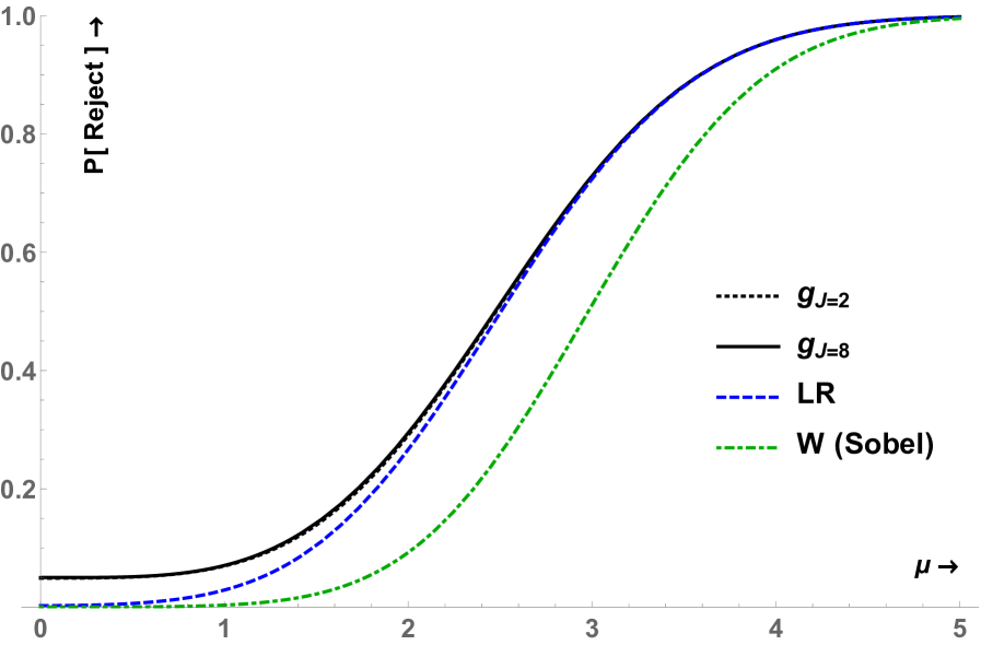
Insistence on similarity can have negative consequences for the power in general, but not here. The power envelope with or without (near) similarity restriction are very close. The power surface of our optimal test is also close. Even the basic test with has very good power in comparison with the Sobel and LR tests and is uniformly better for all values of the noncentrality parameter . In a neighborhood of the origin with it is essentially points higher.
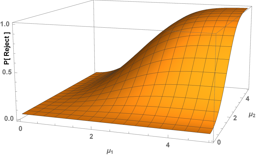
The RP defined in Equation (9) is the NRP if and/or equal (the null hypothesis). When both are non-zero, is false and is the power of the test defined by . Figure 6 illustrates the power in the direction. Power in other directions is also superior to the Wald (Sobel) and LR tests.
There is a straightforward explanation for the additional power. The Wald and LR test both reject far less than near the origin. The critical region can therefore be extended and the power increased without failing the size condition. In the origin the NRPs are close to for the LR and Wald (Sobel) tests. By extending the critical region we can therefore gain almost power without violating the size condition. The LR test has some attractive features including that rejection for a particular implies rejection for larger values of and/or also. This is intuitive since the evidence against the null is increasing. A disadvantage is however that one never rejects when either or is smaller than and this causes extreme conservativeness that can be resolved by adding area to the critical region. It should also be noted that the relevant distribution of the order statistic is quite different from the distribution of the product of two standard normals for or their absolute values.
3.3 Power Envelope
Comparison to the Sobel and LR tests is limited because they both perform very poorly for small values of . The absolute quality, or even near optimality, of the new -test can only be assessed by comparing the power surface of the test to the power envelope, or a tight upper bound thereof, for a class of tests that satisfy appropriate invariance-, size and almost similarity restrictions. Since the exact similar invariant test is objectionable when it exists, we introduce a class of near similar tests with NRPs that deviate less than from the level and an operational (super)class as follows.
Definition 3
The class of near similar boundary functions with and given is defined by:
The class with set containing points under , is defined by:
For the boundary functions in would be similar. We consider in all our numerical examples, but for general the set would be empty according to Theorem 2. For , on the other hand, contains all -based tests that satisfy the size condition. Our interest is in close to , when contains boundaries that are almost similar. The minimum value of for which is not empty is 0 for the mediation problem when , but in general depends on the testing problem considered and larger than if no similar test exists.
The class can be thought of as a discretization of in the sense that a grid of points under the null is considered. It imposes less restrictions and enforces near similarity conditions on a finite number of points only. As a consequence it may contain boundaries that do not satisfy the size condition for points that are not in Obviously since the size and NRP conditions also hold for the points in .
Within the class there is no unique solution. As a consequence one has to choose a boundary function from or in practice from to obtain an operational test. For the construction of the power envelope we can select the test in that maximizes the power against a particular point in the alternative. This test is a Point Optimal Invariant Near Similar (POINS) test. The critical region of this test varies with and no uniformly most powerful test exists within the class . It can be used however, to construct an upper bound for the power envelope.
Definition 4
The power envelope of a near similar invariant test with is defined as:
For a given set of points an upper bound to the power envelope is:
For notational simplicity we have suppressed the dependence on and Since and elements of do not necessarily satisfy the size condition for all parameter values it follows that because fewer conditions are imposed. Choosing a finer grid for will force closer to , at least in the additional points in where the size condition is now required to hold. Also note that the “point” optimal that maximizes power for the point may have undesirable features such as including parts of the axes in the critical region, even though such observations are perfectly in line with the null hypothesis.
We determine numerically for by maximizing the power directly by selecting critical region points in the sample space that maximize the probability of rejection when the true density has parameter , under the side conditions that the NRP for all parameters . The sample space is decomposed into squares and a modern optimization routine is used to determine which squares should be included in the critical or acceptance region in order to maximize the power while at the same time satisfying the approximate similarity condition. This is repeated for a grid of points. So for each point on the grid the POINS critical region is determined and the power recorded. Appendix D gives details of the algorithm and the optimization routine that can deal with a large number of variables and side conditions.
By dropping the near similarity restriction ( in the same algorithm, we can construct a power envelope for nonsimilar tests. The maximal difference from the (higher) nonsimilar power surface is points when power is around showing that the power loss due to the similarity requirement is small. The calculated surface enables us to construct a correctly sized optimal test derived in the next section.
4 The New Mediation Test
Having determined an upper bound to the power envelope, we can determine a -boundary function with a power surface as close as possible to this upper bound. This optimal test is found using the algorithm given in Appendix D. This function is given in Appendix E and R-code is also provided there. For ease of implementation we give values of in Table 1. Figure 7 shows the optimal -boundary test for the mediation problem.
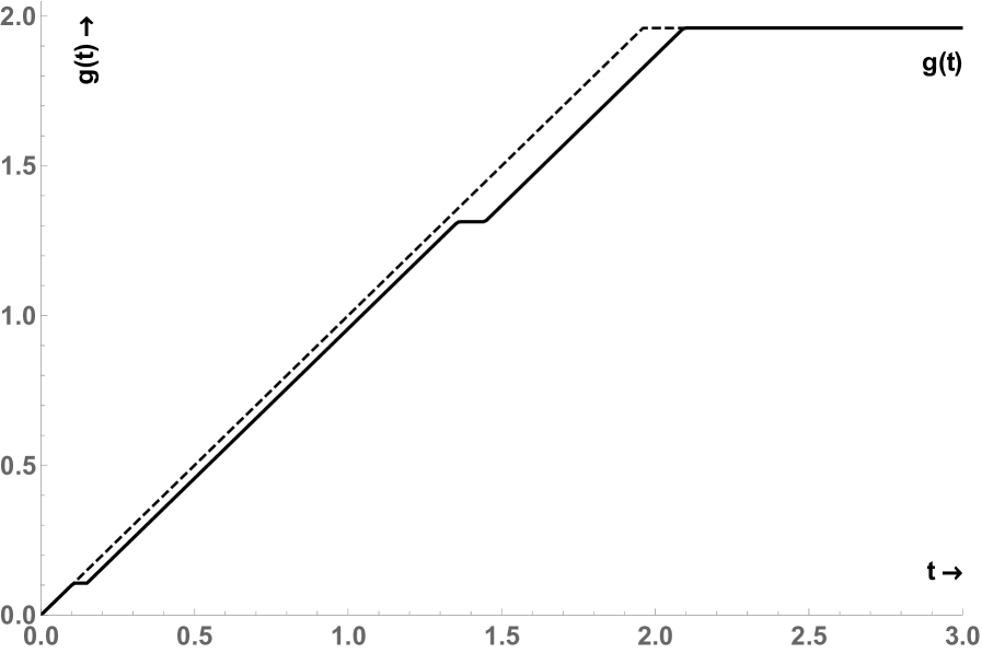

The optimal includes a narrow region close to the line where both -statistics are of the same magnitude. This is expedient for two reasons. First, because mediation requires both and to be non-zero. The best possibility of detecting this is along the line as illustrated by the power surface in Figure 9 showing highest power on the diagonal. The optimal does exclude both -statistics smaller than , unlike the unappealing region of the exact test. Second, the near similarity condition requires additional critical region area in the left corner of the octant because NRPs are particularly low for small parameter values. The increased power is naturally linked to the increase in Type I error, but correct size of a test by definition merely requires that this is not larger than . Nevertheless, size (NRP)/power trade-off exists as well as other compromises that can be assessed using critical region analysis. For instance, it may seem less intuitive that rejection is not monotonic in and since an increase in both and represents increased evidence against the null. The LR and Wald tests are monotonic in this sense, but lead to a reduction in power to nearly zero for small parameter values. No observed value of will ever lie on the horizontal or vertical axis. Any observed is therefore more likely given an alternative parameter value than a value under the null. It is therefore desirable to add area to the LR critical region even if this results in a non-convex critical region or acceptance region. One could cogitate about the very narrow region close to the diagonal and whether the acceptance should not continue along the line further than until e.g. as in Figure 2(b), but the new -boundary is the optimal solution to a well-defined problem.
The narrow region of the optimal is a strict extension of the which itself is strictly larger than the Sobel (Wald) . Since the new test is constructed to satisfy the size condition we have the following:
Theorem 3
The Sobel/Wald test and the LR test are inadmissible.
Proof. hence . The optimal -test has uniformly higher power and is correctly sized by construction.
The NRP as a function of the noncentrality parameter is shown in Figure 8. The difference from is less than and so small that the scale had to be magnified greatly, to an extend that prevents comparison with the LR and Sobel tests in the same graph.
The power of the new -test is very close to the power envelope (upper bound). The maximal difference is . This has important implications. First, the upper bound is tight as claimed earlier. Second, the upper bound of the power envelope and power surface of the -test look almost identical when graphed. Figure 9 therefore shows only the power surface of the optimal -test. Finally, the new -test is optimal for all intents and purposes in a larger class of tests. It is optimal by construction within the class of near similar tests , but given the closeness of its power surface to the (non)similar power envelope, there cannot exist any near similar test that has additional power more than , even if construction is based on a different method. More generally, nonsimilar tests can have points more power, but at the possible cost of odd rejection regions and low power for other parameter values that are not used in the construction of the test. The optimal -test has good properties for all parameter values.
The power surface in Figure 9 shows only the first quadrant of the parameter space of The other three quadrants follow by simple permutations and reflections of the parameters.
5 Application: Educational Attainment and Gender
To illustrate the usage of the new test, we consider the mediation analysis in Alan et al. (2018) on the effect of elementary school teachers’ gender beliefs, either traditional or progressive, on student mathematical and verbal achievements. They exploit the unique institutional features of Turkish data that provides a natural experiment in the random allocation of teachers to schools. Information consists of approximately 4,000 third- and fourth-grade students and their 145 teachers. The data are available in their online appendix. Children are divided into three groups depending on the length of exposure to a participating teacher: “1-year exposure” (at most one year), “2-3 year exposure” (more than one year and at most three years) and “4-year exposure” (at most four years). Alan et al. (2018) consider three potential mediators, but we focus on students’ own gender role beliefs. In the notation of equations (1)-(3), is a dummy whether the teacher is classified as traditional or progressive. The mediating variable is the student’s own belief on gender roles. We focus on the verbal test scores as the dependent variable . Table 2 shows the estimates for the indirect effect for girls based on the full sample and the three exposure groups after controlling for school fixed effects, student characteristics, family characteristics, teacher characteristics, teacher styles and teacher effort.
The results for the full sample are similar to the values shown in Table 5 and Table 6 of Alan et al. (2018), although they use the approach by Imai et al. (2013). We consider three different exposure duration groups. The -ratios of are not significant at the level for more than 1-year exposure. For the 1-year exposure, however, it is significant, but the -ratio of is not. So, the LR test would not find a significant effect and neither does the simulation based method Alan et al. (2018) use. Using the new test, however, we have and , such that and consequently and the proposed test finds the mediation effect significant at the level. The R function in Appendix E can be used if greater precision is desired, e.g. .
| Exposure: | Full | 1-Year | 2-3 Year | 4-Year | |||
|---|---|---|---|---|---|---|---|
| 0.199 | 0.256 | 0.109 | 0.064 | ||||
| -ratio: | 3.140 | 2.052 | 1.065 | 0.513 | |||
| -0.119 | -0.097 | -0.125 | -0.113 | ||||
| -ratio: | -5.343 | -1.941 | -4.163 | -1.931 | |||
| : | -0.024 | -0.025 | -0.014 | -0.007 |
6 Higher Dimensions
In a further empirical illustration below, mediation may be via channels that involve two mediating variables. This requires a multivariate extension of the new test. The necessary invariance and distribution theory was given in Section 2 but a further aspect is the coherency between solutions in different dimensions. Consider the null hypothesis in dimensions. If it were known that then the null hypothesis reduces to This implies that the critical region for the corresponding -statistics should reduce to the solution found for dimensions when is large. For large values of (very small -values) it is essentially known that and are non-zero. The probability of rejection will effectively depend only on the other -values. In two dimensions this means that as the boundary function , which is the one-dimensional solution for testing when In three dimensions it means that the solution must reduce to the -test derived in Section 4. We make this requirement explicit in the definition below.
Definition 5
The -boundary in dimension for the test that rejects if is dimensionally coherent if for each
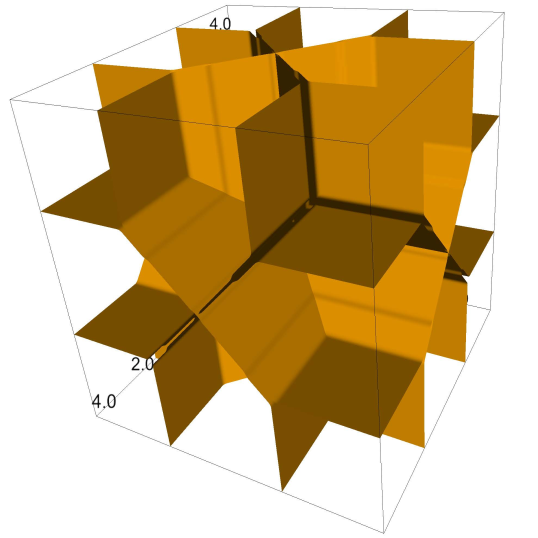
We used a multivariate spline generalization to implement the varying -method based on barycentric coordinates in three dimensions. It resulted in a maximum of points difference from . But imposing dimensional coherency was complicated and the problem suffers from the curse of dimensionality: the dimension of the integral increases with and the number of knots necessary to define impedes optimization. For practical purposes we therefore propose a simple solution that exploits the dimensional coherency inductively and weighs the LR test in dimension with the solution obtained in dimension . First note that one could satisfy the coherency condition in three dimensions by simply rejecting when irrespective of This results in an invalid test however, because it is oversized with a maximum NRP of when . The LR test on the other hand is conservative, in particular near the origin. A practical solution therefore is to use a weighted average between the liberal and conservative boundary. We use weights that depend on the largest absolute -statistic. In particular for
with weight function a linear spline with and . The test rejects if Minimizing deviation ofthe NRP from the significance level and imposing the size restriction, results in a spline with knots:
leading to a maximum of points difference in NRPs from and never exceeding . The solution is shown in Figure 10.
7 Empirical Illustration
For a numerical illustration, we consider the recursive model of union sentiment among southern nonunion textile workers as used by Bollen and Stine (1990). The model:
| (11) |
is a simplified version of McDonald and Clelland (1984) and discussed in some detail by Bollen (1989, p. 82–93). It analyses the direct and indirect effects of tenure and age on union sentiment via deference and/or labor activism. Tenure is measured in log of years working in a particular textile mill and age is measured in years. The variables sentiment towards unions , deference/submissiveness to managers , and support for labor activism , are measures based on 7, 4, and 9 survey questions respectively. The disturbances (, and ) are assumed to be uncorrelated across equations and individuals. When they are normally distributed, ML estimation of the system reduces to OLS applied to each equation separately due to the recursive structure.
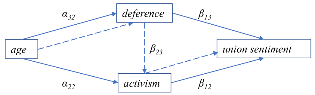
We use a selection of 100 observations out of the original 173 and focus on three alternative theories of the indirect effects from age to union sentiment: two competing parallel effects that the age effect is mediated by increased deference in which case quantifies the indirect effect. The alternative mediation channel is that activism mediates such that is the indirect effect. The third channel is a serial effect that age affects deference, which in turn affects activism, which in turn affects union sentiment such that measures the indirect effect. Figure 11 illustrates the three mediation channels. The OLS estimates of the coefficients of the structural equations and their -statistics are shown in Table 3.
| Estimate | –0.050 | 0.057 | –0.283 | 0.987 | –0.215 | 0.720 |
|---|---|---|---|---|---|---|
| -statistic | –1.902 | 2.709 | –3.582 | 7.120 | –1.838 | 1.777 |
The point estimates of the indirect effects and their -statistics based on the delta method are shown in Table 4. For the -test we need the absolute order statistics, evaluate and compare. For we observe and hence reject. For we have and also reject. Testing the last null hypothesis requires the three-dimensional solution given in Figure 10. We have and do not reject.
| Estimate | Sobel -statistic | -test | |
|---|---|---|---|
The Sobel test with critical value concludes that is significant but does not find enough evidence for the mediation channel. The new -test in contrast, concludes that is also significant. Both -values in this case are smaller than , so the LR test would not reject either. The two -values are of comparable magnitude and the -test finds a significant mediation effect. For implementation of the -test only the relevant -statistics are required. The absolute values are ordered and the smallest value compared with the value of the -function evaluated at the largest absolute -value. This can be looked up in Table 1 (possibly using linear interpolation) or one can use the R code provided in Appendix E.444The bootstrap is a popular alternative for testing mediation. Because of the asymmetry of the distribution involved this is carried out through alternative confidence intervals of the indirect effect. See e.g. MacKinnon et al. (2004) and Preacher and Hayes (2008). The bootstrap is not valid. Simulations we carried out showed that bootstrap tests for mediation based on generally preferred BCa confidence intervals can have sizes of 8% when and higher for smaller.
For both tests draw the same conclusion. The three -values involved are not of comparable magnitude and the -statistics for and are so large that rejecting the null essentially depends on whether is zero. The corresponding absolute -value of is too small to warrant such conclusion.
8 Conclusion
This paper proposes a new near similar more powerful mediation test that is simple to used based on two ordinary -statistics. The mediation problem is empirically extremely important in many different fields. Theoretically we solve an interesting statistical problem which has generated results dating back to Craig (1936) and still continues today with contributions on poor performance of the Wald statistic, construction of similar tests, and hypotheses with singularities. A main theoretical contribution has been the derivation of an exact similar test that is unique within the general class considered (with CR that is topologically simply connected and has weak monotone càdlág boundary). This exact test has unattractive statistical properties, however, leading us to consider a class of nearly similar tests and choose an attractive test within it. By relaxing the strict similarity condition we are able to construct a near similar test that has superior power and avoids the disagreeable properties of the exact similar test and would please even statistically erudite emperors in Perlman and Wu (1999). The new test can also be justified asymptotically under much weaker conditions and other estimation methods.
The new test is constructed using a new general method we propose for constructing tests that are approximately similar. This varying- method considers a flexible critical region boundary and minimizes the difference from the level of the rejection probabilities at a number of points on the boundary of the null hypothesis. Conceptually and practically this was very simple and straightforward to implement. It does not require, as in other approaches, a choice of mixture distribution, nor the construction of least favorable distributions. Numerically it is also attractive in terms of convergence properties and avoids the need for simulations. The appropriate distribution theory for the mediation case and higher dimensional extensions is explicitly given. All our calculations are done using numerical integration using the distribution of the maximal invariant.
The new method is applicable to many other testing problems with nuisance parameters. It is remarkable that this simple method works so well and can deliver substantial improvements. Even the simplest linear interpolation implementation for the mediation hypothesis increases power by almost points when mediation effects are small.
We have calculated a power envelope upper bound for the mediation testing problem that is very tight. Using this result, we were able to construct a test that is optimal within the class of near similar tests. It minimizes the total difference between its power surface and the power envelope bound. It results in a point wise difference less than for all alternative parameter points considered. This implies that the test is practically optimal even if a more general class of possible test construction is considered. A power envelope for nonsimilar tests showed that power loss due to the similarity requirement is minimal since the maximum power loss is less than points (when maximum power is around ).
The optimal -test satisfies the size condition. The critical region is strictly larger than the LR and Wald critical regions and is therefore strictly and uniformly more powerful. The classic tests are therefore not admissible and their bootstrapped variants are not valid. For large values of the standardized coefficients the power difference becomes negligible, but when mediation effects are small or have relatively large standard errors, the power can be close to points higher than these classic -level tests. This has important consequences for empirical work. It enables researcher to prove mediation effects earlier in circumstances that one could not show mediation before due to extreme conservativeness of standard tests near the origin.
Appendix A Theory
A.1 Elementary Relation
Let , , , be vectors of observables in deviations from their means such that , , and disturbance vectors , The model is then:
| (12) | ||||
| (13) |
and the restricted version of Equation (12) with equals:
| (14) |
A.2 Likelihood
The joint density of given is and according to the model:
Hence the log-likelihood: for independent observations equals Equation (5) which can be written as:
and some function of and which is fixed. Since the model is a full exponential model of dimension five following the Koopman-Fisher-Darmois theorem (see Van Garderen (1997)) and is a complete sufficient statistic. The score is analogues to the scores of the two separate regression models since appears in the first equation only, and appears in the second equation only. So:
and the Maximum Likelihood Estimator (MLE) equals the MLE for the two
equations separately:
with and an matrix. The MLE is minimal sufficient and complete because it is a bijective transformation of which is a minimal sufficient and complete statistic.
A.3 Classic Tests
Wald test. Under . Then and evaluated at the (unrestricted) MLE equals The Wald test therefore becomes:
The Sobel test equals and is usually expressed as the square root of the first term in the second line:.
LR test. The maximum value of the log-likelihood can be expressed in terms of the OLS residual sum of squares in the usual way for the first and second equation, and respectively:
Denote the restricted residual sums of squares by when , when and the restricted maximized log-likelihoods by:
The LR test of the full model with five parameters, against the model with the single restriction equals:
Analogously the LR test for equals:
The likelihood ratio test for and/or uses the maximized log-likelihood under the alternative (the same in both cases) and under the null, which means minimizing over and and hence:
which is equivalent to rejecting for large values of:
Appendix B Invariance
When testing the no-mediation hypothesis the parameters are nuisance parameters and their values have no influence on whether the null is true or not. Hillier et al. (2021) shows that is maximal invariant with respect to an appropriate group of transformations that leaves the testing problem invariant and provides justification for restricting attention to the two -statistics. These exact invariance results provide a strong justification for restricting attention to the two -statistics for any sample size, finite or asymptotically, since it is natural to restrict the problem to procedures that are scale invariant and do not depend on
The testing problem has further invariance properties. The problem is invariant to changing the signs (reflections) of and or permuting them. This leads to maximal invariants with a sample and parameter space that is only part of .
Proof. (of Theorem 1) is obviously invariant to changes in sign and permutation as a consequence of the absolute values and subsequent sorting. It is a maximal invariant because any two and such that can only hold if is a permutation of with a number of sign changes. Hence there will exist a transformation s.t. The same argument holds for since the group of transformations on the parameter space is the same as on the sample space. That the distribution of depends only on is a property of a maximal invariant.
Lemma 1 gives an explicit expression that further shows that the distribution is invariant under the .
Appendix C Proof of Theorem 2
The proof exploits the symmetries of the problem and the completeness of the normal distribution. We therefore consider the sample space of in , rather than the octant that is the sample space of the maximal invariant. The proof is constructive. It shows how to construct a monotonic weakly increasing function with steps, when is an integer. If is not an integer then it cannot satisfy the condition that the final step equals the asymptotic value which is the normal critical value and determined by letting There are two trivial solutions. First, if then and the test always rejects, leading to an NRP of for all parameter values. The other trivial solution is such that and the test would never reject and the NRP is 0% for all .
Proof. Symmetry of the problem implies for the boundary function and So we only define for and The boundary function is weakly monotonically increasing by assumption, but may be a step function. If is a step function then it has no ordinary inverse but we can define its generalized inverse as:
(cf. quantile function e.g. Van der Vaart (2000, p.304)). This definition of with strict inequality is chosen such that a necessary condition for similarity may hold.
-
1.
For any finite constant we have
and rejection only depends on when . Hence such that:
Monotonicity of implies and we follow the convention that
-
2.
The null rejection probability as a function of equals:
-
3.
Similarity requires . Hence
(15) -
4.
Completeness of the normal distribution with mean implies the condition
(16) We will show that this leads to a step function and the proof iteratively determines the stepping points and step sizes, illustrated in the Figure 3.
-
5.
Starting at we have by definition, but for a generalized inverse there are two possibilities:
-
(a)
For condition (16) implies: only holds if . In this case can only occur if and the test never rejects.
-
(b)
. In this case
-
i.
and imply and
-
ii.
and imply
-
iii.
and in turn imply but so
-
iv.
-
v.
because implies and the result follows by the uniqueness of the inverse of .
-
i.
-
(a)
-
6.
This argument can now be repeated.
-
(a)
In implies and As in 5.b.i) ii) iii) and
-
(b)
After repetitions of this argument we obtain a step function:
-
(a)
-
7.
An exact similar test only exists if is an integer.
-
(a)
If is an integer such that then and . The resulting step-function is constructed such that for all . The NRP equals for all
So an exact similar test exists if is an integer. -
(b)
If is not an integer then define (entier or floor function) and the remainder such that So . After iterations of the argument in Step 5 gives Similarly iterations give: . Therefore the step-function does not have which is the requirement for the NRP to equal as Further note that the next step after iterations has so we cannot apply to obtain the next boundary point.
So no similar -test exists if is not an integer.
-
(a)
Appendix D Algorithms
The construction of the optimal -test is in two steps. The first step is a basic implementation of the general varying- method. This generates a near similar test that deviates less than points from We use this as a starting value for determining an upper bound to the power envelope. The second step is using this upper bound to derive an optimal -test that minimizes the distance between the power surface and the power envelope for tests in . Implementation of the varying- method.
Basic -function algorithm
-
1.
Define nonparametrically as a linear spline defined by knots i.e. by values on a grid of points The first and last knots are fixed at and respectively, so there are knots to be chosen. One of those knots is chosen such that the LR boundary can be constructed as initializing function. For points not on the grid, is obtained by linear interpolation, and for
-
2.
The criterion function is the accumulated NRP deviation from as measured by a quadratic loss function over a grid of points with and
-
3.
Minimize by varying :
-
(a)
Initialize with knots which is the function corresponding to the LR boundary. The first and last knot are fixed and the middle one is varied when optimizing .
-
(b)
For given calculate the NRPs by numerical integration for the grid of noncentrality parameter points under the null, with and calculate
-
(c)
Vary by changing knots and minimize the criterion function , subject to:
-
i.
: monotonicity and limited increase
-
ii.
: logical restriction since maximal invariant is absolute order statistic and
-
iii.
: dimensional coherence requires reduction to one-dimensional solution (see Section 6)
-
i.
-
(d)
Increase the number of knots and iterate until convergence.
-
(a)
Comments
-
1.
We set for because for large enough it is essentially known that and the rejection depends only on whether is rejected. The corresponding critical value for based on the normal distribution is the usual as
-
2.
For small there are big gains in reducing the deviation from by varying the knots and also by increasing see Figure 5.
-
3.
The number of points to check similarity was chosen to be : 60 points equally spaced between 0 and 6, and 16 points equally spaced between 6 and 20. This imposes 152 side conditions. Step 3(c) imposes a further restrictions approximately for every choice of , and about when
-
4.
We have actually used as a side condition and iterated to find the smallest that yields a feasible solution.
Optimal -function
In order to find the optimal , we minimize the sum of differences between ’s power surface and the power envelope on a grid of points, subject to the size and -similarity conditions. We impose monotonicity and, since by definition of the absolute order statistic ,we logically restrict to .
Optimal -function algorithm
-
1.
Define nonparametrically as a linear spline defined above.
-
2.
Define the criterion function as the accumulated power difference over the triangular grid of points
-
3.
Minimize by varying :
-
(a)
Initialize with equal to the LR boundary or the previously determined basic -function.
-
(b)
For given calculate by numerical integration.
-
(c)
Vary by changing knots and minimize the criterion function , subject to:
-
i.
: near similarity and size restrictions
-
ii.
: monotonicity,
-
iii.
limited increase and derivative,
-
iv.
: logical restriction since argument is absolute order statistic,
-
v.
: dimensional coherence.
-
i.
-
(d)
Increase the number of knots and iterate until convergence.
-
(a)
The basic implementation algorithm solved the optimal -boundary by minimizing Once is determined, the current algorithm is akin to solving a dual problem that uses for the inequality restrictions and maximizes power. It minimizes the total difference from the power envelope.
Power Envelopes
We calculate two power envelopes: one for near similar tests in and a second for nonsimilar tests. The algorithm for calculating the power envelope is related to Chiburis (2009) and implemented in Julia, see Bezanson et al. (2017), using Gurobi, an optimization package that can handle many side restrictions; see Gurobi Optimization (2021). We maximize power subject to size and near similarity restrictions on a grid of parameter points under the null: for . The upper bounds ensure correct size, at least for the points considered. The lower bounds constitute the near similarity restriction. The power envelope is obtained by repeating this maximization on a grid of points under the alternative.
For the nonsimilar power envelope we can discard the lower bound restrictions . The power can only increase (or remain the same) and the difference between the two different power envelopes is the power loss one suffers from insisting on similarity. This turns out to be less than points and it should be stressed that this overstates the loss since no single test achieves the power envelope.
Denote the parameter space for the ordered absolute noncentrality parameter
We will use a bounded (triangular) subset of this octant defined as
and
partitioned it into a null and alternative parameter set
and
respectively.
Analogously define the sample space of the maximal invariant/absolute order
statistic as . Very large values of and are of limited interest and for computational purposes we can
restrict ourselves to a bounded triangular subset of the sample space:
Power Envelope Algorithm
-
1.
Discretize into points under
-
2.
Discretize by choosing a triangular array of points under
-
3.
Partition into squares with such that and
-
4.
Under for calculate
-
5.
For each choose under the alternative. For this :
-
(a)
Calculate for each
-
(b)
Determine the critical region to maximize the power
by selecting indicators equal to 1 if is part of the critical region, or 0 if part of the acceptance region, subject to the near similarity and size restrictions on the NRPs:
-
(a)
Comments. Optimizer: Gurobi: each square has lengths Hence cardinality of . For power calculations we use for a regular grid with . For size and near similarity restrictions we use and for near similarity
Appendix E -Function R Code
R Code
g <- function(t){
tabs=abs(t)
x - c(0., 0.1, 0.11, 0.13, 0.14, 0.15, 1.35, 1.36, 1.37, 1.44, 1.45, 2.05, 2.06, 2.07, 2.08, 2.09, 2.1)
y - c(0., 0.1, 0.106723, 0.106723, 0.106724, 0.106724, 1.30583, 1.31286, 1.3131, 1.3131, 1.3175, 1.9175, 1.9275, 1.9375, 1.9475, 1.9575, 1.95996)
ifelse(tabs=2.1,1.95996,approx(x,y,xout=tabs)$y)
}
References
- Alan et al. (2018) Alan, S., S. Ertac, and I. Mumcu (2018). Gender stereotypes in the classroom and effects on achievement. Review of Economics and Statistics 100(5), 876–890.
- Alwin and Hauser (1975) Alwin, D. F. and R. M. Hauser (1975). The decomposition of effects in path analysis. American sociological review 40, 37–47.
- Andrews et al. (2006) Andrews, D. W. K., M. J. Moreira, and J. H. Stock (2006). Optimal two-sided invariant similar tests for instrumental variables regression. Econometrica 74(3), 715–752.
- Andrews et al. (2008) Andrews, D. W. K., M. J. Moreira, and J. H. Stock (2008). Efficient two-sided nonsimilar invariant tests in iv regression with weak instruments. Journal of Econometrics 146(2), 241–254.
- Andrews and Ploberger (1994) Andrews, D. W. K. and W. Ploberger (1994). Optimal tests when a nuisance parameter is present only under the alternative. Econometrica 62(6), 1383–1414.
- Baron and Kenny (1986) Baron, R. M. and D. A. Kenny (1986). The moderator–mediator variable distinction in social psychological research: Conceptual, strategic, and statistical considerations. Journal of personality and social psychology 51(6), 1173.
- Berger (1989) Berger, R. L. (1989). Uniformly more powerful tests for hypotheses concerning linear inequalities and normal means. Journal of the American Statistical Association 84(405), 192–199.
- Bezanson et al. (2017) Bezanson, J., A. Edelman, S. Karpinski, and V. B. Shah (2017). Julia: A fresh approach to numerical computing. SIAM review 59(1), 65–98.
- Bollen and Stine (1990) Bollen, K. and R. Stine (1990). Direct and indirect effects: Classical and bootstrap estimates of variability. Sociological methodology 20, 115–140.
- Bollen (1989) Bollen, K. A. (1989). Structural equations with latent variables. John Wiley & Sons.
- Chiburis (2009) Chiburis, R. C. (2009). Approximately most powerful tests for moment inequalities. In Essays on Treatment Effects and Moment Inequalities, Chapter 3. Ph.D. thesis, Department of Economics, Princeton University.
- Coletti et al. (2005) Coletti, A. L., K. L. Sedatole, and K. L. Towry (2005). The effect of control systems on trust and cooperation in collaborative environments. The Accounting Review 80(2), 477–500.
- Craig (1936) Craig, C. C. (1936). On the frequency function of xy. The Annals of Mathematical Statistics 7(1), 1–15.
- Drton (2009) Drton, M. (2009). Likelihood ratio tests and singularities. The Annals of Statistics 37(2), 979–1012.
- Drton and Xiao (2016) Drton, M. and H. Xiao (2016). Wald tests of singular hypotheses. Bernoulli 22(1), 38–59.
- Dufour et al. (2017) Dufour, J.-M., E. Renault, and V. Zinde-Walsh (2017). Wald tests when restrictions are locally singular. Technical report, arxiv.org/abs/1312.0569v1.
- Elliott et al. (2015) Elliott, G., U. K. Müller, and M. W. Watson (2015). Nearly optimal tests when a nuisance parameter is present under the null hypothesis. Econometrica 83(2), 771–811.
- Frewen et al. (2013) Frewen, P. A., V. D. Schmittmann, L. F. Bringmann, and D. Borsboom (2013). Perceived causal relations between anxiety, posttraumatic stress and depression: extension to moderation, mediation, and network analysis. European journal of psychotraumatology 4(1), 20656.
- Glonek (1993) Glonek, G. F. V. (1993). On the behaviour of wald statistics for the disjunction of two regular hypotheses. Journal of the Royal Statistical Society: Series B (Methodological) 55(3), 749–755.
- Guggenberger et al. (2019) Guggenberger, P., F. Kleibergen, and S. Mavroeidis (2019). A more powerful subvector anderson rubin test in linear instrumental variables regression. Quantitative Economics 10(2), 487–526.
- Gurobi Optimization (2021) Gurobi Optimization, L. (2021). Gurobi optimizer reference manual.
- Heckman and Pinto (2015a) Heckman, J. and R. Pinto (2015a). Causal analysis after haavelmo. Econometric Theory 31(1), 115–151.
- Heckman and Pinto (2015b) Heckman, J. and R. Pinto (2015b). Econometric mediation analyses: Identifying the sources of treatment effects from experimentally estimated production technologies with unmeasured and mismeasured inputs. Econometric reviews 34(1-2), 6–31.
- Hillier et al. (2021) Hillier, G. H., K. J. Van Garderen, and N. P. A. Van Giersbergen (2021). Improved tests for mediation. Mimeo.
- Huber (2020) Huber, M. (2020). Mediation analysis. Handbook of Labor, Human Resources and Population Economics, 1–38.
- Imai et al. (2010) Imai, K., L. Keele, and T. Yamamoto (2010). Identification, inference and sensitivity analysis for causal mediation effects. Statistical science 25(1), 51–71.
- Imai et al. (2013) Imai, K., D. Tingley, and T. Yamamoto (2013). Experimental designs for identifying causal mechanisms. Journal of the Royal Statistical Society: Series A (Statistics in Society) 176(1), 5–51.
- Imbens (2020) Imbens, G. W. (2020). Potential outcome and directed acyclic graph approaches to causality: Relevance for empirical practice in economics. Journal of Economic Literature 58(4), 1129–79.
- Lehmann and Romano (2005) Lehmann, E. L. and J. P. Romano (2005). Testing statistical hypotheses (3 ed.). Springer Science & Business Media.
- MacKenzie et al. (1986) MacKenzie, S. B., R. J. Lutz, and G. E. Belch (1986). The role of attitude toward the ad as a mediator of advertising effectiveness: A test of competing explanations. Journal of marketing research 23(2), 130–143.
- MacKinnon et al. (2002) MacKinnon, D. P., C. M. Lockwood, J. M. Hoffman, S. G. West, and V. Sheets (2002). A comparison of methods to test mediation and other intervening variable effects. Psychological methods 7(1), 83.
- MacKinnon et al. (2004) MacKinnon, D. P., C. M. Lockwood, and J. Williams (2004). Confidence limits for the indirect effect: Distribution of the product and resampling methods. Multivariate behavioral research 39(1), 99–128.
- McDonald and Clelland (1984) McDonald, J. A. and D. A. Clelland (1984). Textile workers and union sentiment. Social Forces 63(2), 502–521.
- Moreira and Mourão (2016) Moreira, M. J. and R. Mourão (2016). A critical value function approach, with an application to persistent time-series. arXiv preprint arXiv:1606.03496.
- Perlman and Wu (1999) Perlman, M. D. and L. Wu (1999). The emperor’s new tests. Statistical Science 14(4), 355–369.
- Preacher and Hayes (2008) Preacher, K. J. and A. F. Hayes (2008). Asymptotic and resampling strategies for assessing and comparing indirect effects in multiple mediator models. Behavior research methods 40(3), 879–891.
- Sobel (1982) Sobel, M. E. (1982). Asymptotic confidence intervals for indirect effects in structural equation models. Sociological methodology 13, 290–312.
- Van der Vaart (2000) Van der Vaart, A. W. (2000). Asymptotic statistics, Volume 3. Cambridge university press.
- Van Garderen (1997) Van Garderen, K. J. (1997). Curved exponential models in econometrics. Econometric Theory 13(6), 771–790.
- Van Garderen and Van Giersbergen (2021) Van Garderen, K. J. and N. P. A. Van Giersbergen (2021). Bootstrapping mediation tests. Mimeo.
- Van Giersbergen (2014) Van Giersbergen, N. P. A. (2014). Inference about the indirect effect: a likelihood approach. Technical report, University of Amsterdam, UvA-Econometrics Discussion Papers 2014/10.
- Vaughan and Venables (1972) Vaughan, R. J. and W. N. Venables (1972). Permanent expressions for order statistic densities. Journal of the Royal Statistical Society: Series B (Methodological) 34(2), 308–310.