xx \jmlryear2020 \jmlrworkshopACML 2020
A New Accelerated Stochastic Gradient Method with Momentum
Abstract
In this paper, we propose a novel accelerated stochastic gradient method with momentum, which momentum is the weighted average of previous gradients. The weights decays inverse proportionally with the iteration times. Stochastic gradient descent with momentum (Sgdm) use weights that decays exponentially with the iteration times to generate an momentum term. Using exponentially decaying weights, variants of Sgdm with well designed and complicated formats have been proposed to achieve better performance. The momentum update rules of our method is as simple as that of Sgdm. We provide theoretical convergence properties analyses for our method, which show both the exponentially decay weights and our inverse proportionally decay weights can limit the variance of the moving direction of parameters to be optimized to a region. Experimental results empirically show that our method works well with practical problems and outperforms Sgdm, and it outperforms Adam in convolutional neural networks.
keywords:
exponential decaying rate weight, gradient descent, inverse proportional decay rate weight, momentum1 Introduction
A stochastic optimization problem can be consider as minimizing a differentiable function using stochastic gradient descent (SGD) optimizer over a data set which has samples. Function , in the empirical risk format, can be written as , where is the realization of with the th sample. Given the initial and a stepsize , the optimizer iterates with the following rule
| (1) |
until reaches a predefined state. The vector is the stochastic gradient of , which gradient satisfies and has bounded variance Bottou et al. (2018). For large-scale data sets, the computational complexity of iterating with full gradient is unacceptable. It is more efficient to measure a single component gradient , where is the index of the uniformly selected sample from the samples, and move in the noisy direction , than to move in the full gradient direction with a bigger stepsize Ward et al. (2019); Bottou et al. (2018). However, choosing a feasible and suitable stepsize schedule is difficult. According to the work of Robbins and Monro Robbins and Monro (1951), the stepsize schedule should satisfy
| (2) |
to make . This constraint makes full gradient descent methods converge slower than stochastic SGD methods.
Methods using gradients in previous iterations as momentum terms have been proposed to accelerate the convergence and show great benefits Kingma and Ba (2014); Leen and Orr (1993). Yet, theoretical analyses of those method in stochastic settings are elusive, and the ways to generate the momentum term from previous gradients can be revised.
1.1 Stochastic Gradient Methods With Momentum
Stochastic gradient descent methods with momentum (Sgdm) update parameter with
| (3) |
where is called a momentum term, and Sgdm updates the momentum term with
| (4) |
If is a constant, then we call it a exponentially decay rate. With (4), we can rewrite the update rule (3) as
| (5) |
which shows that the moving direction here is a weighted average of all gradients, with exponential decay weights. We denote the weighted average of gradients as . It is believed that the momentum term can reduce the variance Sutskever et al. (2013). Using a exponential decay rate is common and effective. According our following analyses, a exponential decay rate can limit the variance of to a region which determined by the constant .
Main Contribution First, we proposed a novel stochastic gradient descent method with inverse proportional decay rate momentum, which method dynamically adjusts the momentum to match the convergence of the stochastic optimization problem. Besides, our rigorous analyses prove that both the simple SGDM and our novel momentum term can limit the variance to a region (Theorem 3.4,Theorem 3.6). We list out two main theorems (informally) in the following.
For a differential function with -Lipschitz gradient and the variance of gradient is limited, Theorem 3.4 implies that the momentum term with exponentially decay weights can limit the variance of
Theorem 3.6 implies that the momentum term with our inverse proportional decay weights can limit the variance of
Extensive experiments in Section 4 shows that the robustness of our method extends from linear regression to practical model in deep learning problems.
1.2 Previous Work
Momentum method and its use within optimization problems has been studied extensively Sutskever et al. (2013); Orr (1996); Leen and Orr (1993). The classical momentum (CM) method Polyak (1964) accumulates a decaying sum of the previous updates of parmeter into a momentum term using equation (4) and updates with (3). CM uses constant hyperparameter and learning rate . With this method, one can see that the steps tend to accumulate contributions in directions of persistent descent, while directions that oscillate tend to be cancelled, or at least remain small Bottou et al. (2018). Thus, this method can make optimization algorithms move faster along dimensions of low curvature where the update is small and its direction is persistent and slower along turbulent dimensions where the update usually significantly changes its direction Sutskever et al. (2013). The adaptive momentum method in Leen and Orr (1993) uses decaying learning rate and adaptive , where is the network input at time .
1.3 Our Method
Our method updates with
| (6) |
and it updates the momentum term with
| (7) |
where
| (8) |
The hyperparameter is a predefined constant. Thus we can rewrite the updating rules (6),(7), and (8) as
We denote the moving direction of as .
We use the same stepsize as shown in (adam)
| (9) |
And it is straightforward that .
2 Algorithm
See Algorithm 1 for the pseudo-code of our proposed algorithm. We denote as a risk function with noise, which is differentiable with respect to parameters . The optimization problem is to minimize the expected risk function with respect to parameters . We denote as the realizations of the risk function at subsequent iterations . Let be the gradient of with respect to in the th iteration.
Our algorithm updates weighted averages of the previous gradients, denoted as . The hyper-parameter control the decay rates of the weighted averages. We initialize as a vector with all 0 elements.
3 Convergence Analysis
In this section, we show that the momentum term could reduce the variance of stochastic directions along the iterations progress. A fixed exponential decay factor and a changing factor can both limit the variance within a small range.
Let us begin with a basic assumption of smoothness of the objective function.
Assumption 3.1 (Lipschitz-continuous gradients)
The objective function is continuously differentiable and the gradient function of , namely, , is Lipschitz continuous with Lipschitz constant , i.e.,
Assumption 3.1 is essential for convergence analyses of most gradient-based methods, which ensures that the gradient of does not change arbitrarily quickly with respect to the parameter vector . Based on Assumption 3.1, we have
| (10) |
which inequality holds for all .
Proof 3.1.
Using Assumption 3.1, we have
from which the desired result follows.
3.1 Variance Analysis
We first consider a fixed decay factor , which is used in many simple stochastic gradient descent methods with momentum.
Assumption 3.2
The objective function F and stochastic gradient satisfy for all , there exist scalars and such that
Proof 3.3.
According to Assumption 3.1, there is a diagonal matrix with such that
where ; and by further noting that , we have
as claimed.
Theorem 3.4 (a fixed decay factor).
Proof 3.5.
For the SGDM updating strategy, we have direction vector
Hence, along with Assumption 3.2, we obtain
Notice that
Since decays to as increases for , so the variance of could be finally reduced to
Theorem 3.6 (a changing decay factor).
Proof 3.7.
4 Experiments
To compare the performance of the proposed method with that of other methods, we investigate different popular machine learning models, including logistic regression, multi-layer fully connected neural networks and deep convolutional neural networks. Experimental results show that our novel momentum term can efficiently solve practical stochastic optimization problems in the field of deep learning and outperforms other methods in deep convolutional neural networks.
In our experiments, we use the same parameter initialization strategy for different optimization algorithms. The values of hyper-parameters are selected, based on results, from the common used settings, respectively.
4.1 Experiment: Logistic Regression
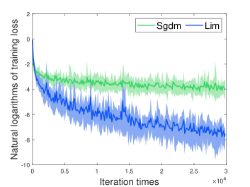
We evaluate the two methods (saying Sgdm, and our method), on two multi-class logistic regression problems using the MNIST dataset without regularization. Logistic regression is suitable for comparing different optimizers for its simple structure and convex objective function. In our experiments, we set the stepsize , where is the current iteration times. The logistic regression problems is to classify the class label directly on the image matrix.
[] \subfigure[]
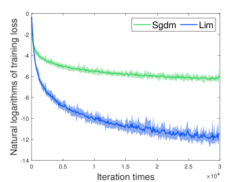
We compare the performance of our method (Lim for short) to optimize the logistic regression problem with that of Sgdm using a minibatch size of 128. According to Fig. 1, we found that our method converges faster than Sgdm.
4.2 Experiment: Multi-layer Fully Connected Neural Networks
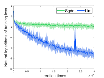
Multi-layer neural networks are powerful models with non-convex objective functions. We empirically found that our method outperforms Sgdm. In our experiments, the multi-layer neural network models are consistent with that in previous publications, saying a neural network model with two or three fully connected hidden layers with 1000 hidden units each and ReLU activation are used for this experiment with a minibatch size of 128.
[] \subfigure[]
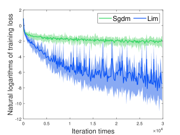
We investigate the two optimizers using the standard deterministic cross-entropy objective function without regularization. According to Fig. 2, we found that our method outperforms Sgdm by a large margin.
4.3 Experiment: Deep Convolutional Neural Networks
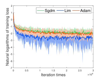
Deep convolutional neural networks (CNNs) have shown considerable success in practical machine learning tasks, e.g. computer vision tasks and natural language procession tasks. Our CNN architectures has three or two alternating stages of convolution filters and max pooling with stride of 2, each followed by a fully connected layer of 1000 units with RLeU activations. We pre-process the input image with whitening imply drop out noise to the input layer and fully connected layer. The minibatch size is also set to 128.
[] \subfigure[]
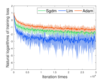
We investigate the three optimizers using the standard deterministic cross-entropy objective function. According to Fig. 3, we found that our method converge faster than Adam and Sgdm.
5 Conclusion
In this paper, we introduced a computationally efficient algorithm for gradient-based stochastic optimization problems. The updating strategies of the proposed method enjoys the simplicity of the original SGD with momentum but utilizes the momentum more efficiently than SGD with momentum. Our method is designed for machine learning problems with large scale data sets and non-convex optimization problems, where is hard for stochastic optimizers to achieve linear converge speed. The experiment results confirm our theoretical analysis on its convergence property and show that our method can solve practical optimization problems efficiently. Overall, we found that our method is a robust and well-suited method to a wide range of non-convex optimization problems in the field of machine learning.
References
- Bottou et al. (2018) Léon. Bottou, Frank E. Curtis, and Jorge. Nocedal. Optimization methods for large-scale machine learning. SIAM Review, 60(2):223–311, 2018.
- Kingma and Ba (2014) Diederik P. Kingma and Jimmy Ba. Adam: A Method for Stochastic Optimization. arXiv e-prints, page arXiv:1412.6980, Dec 2014.
- Leen and Orr (1993) Todd K. Leen and Genevieve B. Orr. Optimal stochastic search and adaptive momentum. In Proceedings of the 6th International Conference on Neural Information Processing Systems, NIPS’93, page 477–484, San Francisco, CA, USA, 1993. Morgan Kaufmann Publishers Inc.
- Orr (1996) Genevieve Beth Orr. Dynamics and Algorithms for Stochastic Search. PhD thesis, USA, 1996.
- Polyak (1964) B.T. Polyak. Some methods of speeding up the convergence of iteration methods. USSR Computational Mathematics and Mathematical Physics, 4(5):1 – 17, 1964.
- Robbins and Monro (1951) Herbert Robbins and Sutton Monro. A stochastic approximation method. Ann. Math. Statist., 22(3):400–407, 09 1951.
- Sutskever et al. (2013) Ilya Sutskever, James Martens, George Dahl, and Geoffrey Hinton. On the importance of initialization and momentum in deep learning. In Proceedings of the 30th International Conference on International Conference on Machine Learning - Volume 28, ICML’13, page III–1139–III–1147. JMLR.org, 2013.
- Ward et al. (2019) Rachel Ward, Xiaoxia Wu, and Léon Bottou. Adagrad stepsizes: sharp convergence over nonconvex landscapes. In Proceedings of the 36th International Conference on Machine Learning, ICML 2019, 9-15 June 2019, Long Beach, California, USA, pages 6677–6686, 2019.