A new approach to QCD final-state evolution in processes with massive partons
Abstract
We present an algorithm for massive parton evolution which is based on the differentially accurate simulation of soft-gluon radiation by means of a non-trivial azimuthal angle dependence of the splitting functions. The kinematics mapping is chosen such as to to reflect the symmetry of the final state in soft-gluon radiation and collinear splitting processes. We compute the counterterms needed for a fully differential NLO matching and discuss the analytic structure of the parton shower in the NLL limit. We implement the new algorithm in the numerical code Alaric and present a first comparison to experimental data.
I Introduction
The production and evolution of massive partons are an important aspect of collider physics, and they play a particularly prominent role at the Large Hadron Collider at CERN. Key measurements and searches, such as and double Higgs boson production, involve final states with many -jets. The success of the LHC physics program therefore depends crucially on the modeling of heavy quark processes in the Monte-Carlo event generators used to link theory and experiment. With the high-luminosity phase of the LHC approaching fast, it is important to increase the precision of these tools in simulations involving massive partons.
Heavy quark and heavy-quark associated processes have been investigated in great detail, both from the perspective of fixed-order perturbative QCD and using resummation, see for example Mangano et al. (1992); Bonciani et al. (1998); Cacciari et al. (2004, 2012). Various proposals were made for the fully differential simulation in the context of particle-level Monte Carlo event generators Norrbin and Sjöstrand (2001); Gieseke et al. (2003); Schumann and Krauss (2008); Gehrmann-De Ridder et al. (2012). Recently, a new scheme was devised for including the evolution of massive quarks in the initial state of hadron-hadron and lepton-hadron collisions Krauss and Napoletano (2018). In this manuscript, we will introduce an algorithm for the final-state evolution and matching in heavy-quark processes, inspired by the recently proposed parton-shower model Alaric Herren et al. (2022). The soft components of the splitting functions are derived from the massive eikonal and are matched to the quasi-collinear limit using a partial fractioning technique. In contrast to the method of Catani et al. (2002); Schumann and Krauss (2008), we partial fraction the complete soft eikonal, leading to strictly positive splitting functions and thus keeping the numerical efficiency of the Monte-Carlo algorithm at a maximum. We also propose to use a kinematic mapping for the collinear splitting of gluons into quarks that treats the outgoing particles democratically. This algorithm can be extended to any purely collinear splitting (i.e., after subtracting any soft enhanced part of the splitting functions) while retaining the NLL precision of the evolution. Our algorithm does not account for the effect of spin correlations.
Multi-jet merging and matching of parton-shower simulations to NLO calculations in the context of heavy-quark production were discussed, for example, in Mangano et al. (2002); Frixione et al. (2003, 2007); Höche et al. (2013). The NLO matching is typically fairly involved, because of the complex structure and partly ambiguous definition of the infrared counterterms. In this publication, we compute the integrated counterterms for our new parton-shower model, making use of recent results for angular integrals in dimensional regularization Lyubovitskij et al. (2021). This calculation provides the remaining counterterms needed for the matching of the Alaric parton-shower model at NLO QCD. We will discuss the extension to initial-state radiation in a future publication.
This paper is structured as follows: Section II briefly reviews the construction of the Alaric parton-shower model and generalizes the discussion to massive particles. Section III introduces the different kinematics mappings. Section IV discusses the general form of the phase-space factorization and provides explicit results for processes with soft radiation and collinear splitting. The computation of integrated infrared counterterms is presented in Sec. V. Section VI discusses the impact of the kinematics mapping on sub-leading logarithms, and Sec. VII provides first numerical predictions for hadrons. Section VIII contains an outlook.
II Soft-collinear matching
We start the discussion by revisiting the singularity structure of -parton QCD amplitudes in the infrared limits. If two partons, and , become quasi-collinear, the squared amplitude factorizes as
| (1) |
where the notation indicates that parton is removed from the original amplitude, and where is the progenitor of partons and . The functions are the spin-dependent, massive DGLAP splitting functions, which depend on the momentum fraction of parton with respect to the mother parton, , and on the helicities Dokshitzer (1977); Gribov and Lipatov (1972); Lipatov (1975); Altarelli and Parisi (1977); Catani et al. (2001, 2002). For the remainder of this work, we will use only the spin-averaged splitting functions.
In the limit that gluon becomes soft, the squared amplitude factorizes as Bassetto et al. (1983)
| (2) |
where and are the color insertion operators defined in Bassetto et al. (1983); Catani and Seymour (1997). In the remainder of this section, we will focus on the eikonal factor, , for massive partons and how it can be re-written in a suitable form to match the spin-averaged splitting functions in the soft-collinear limit. The eikonal factor is given by
| (3) |
Following Refs. Webber (1986); Herren et al. (2022), we split Eq. (3) into an angular radiator function, and the gluon energy
| (4) |
The parton velocity is defined as and is frame dependent. When we label velocities by particle indices in the following, it is implicit that they are computed in the frame of a time-like momentum . In this reference frame they reduce to the relative velocity , where
| (5) |
For convenience, we also introduce the velocity four-vector
| (6) |
When this vector is labeled by a single particle index only, it again refers to the four-velocity of that particle in the frame of , for example . When partial fractioning Eq. (4), we aim at a positive definite result in order to maintain the interpretation of a probability density and, with it, the high efficiency of the unweighted event generation in a parton shower. Following the approach of Ref. Herren et al. (2022), we obtain
| (7) |
The partial fractioned angular radiator function can be written in a more convenient form using the velocity four-vectors. We find an expression that makes the matching to the -collinear sector manifest
| (8) |
In the quasi-collinear limit for partons and , we can write the eikonal factor in Eq. (3) as Catani et al. (2001, 2002)
| (9) |
This can be identified with the leading term (in ) of the DGLAP splitting functions , where 111 Note that in contrast to standard DGLAP notation, we separate the gluon splitting function into two parts, associated with the soft singularities at and .
| (10) |
To match the soft to the collinear splitting functions, we therefore replace
| (11) |
where the two contributions to the gluon splitting function are treated as two different radiators Höche and Prestel (2015). As in the massless case, this substitution introduces a dependence on a color spectator, , whose momentum defines a direction independent of the direction of the collinear splitting Herren et al. (2022). In general, this implies that the splitting functions which were formerly dependent only on a momentum fraction along this direction, now acquire a dependence on the remaining two phase-space variables of the new parton. It is convenient to define the purely collinear remainder functions
| (12) |
They can be implemented in the parton shower using collinear kinematics, while maintaining the overall NLL precision of the simulation. This will be discussed further in Sec. VI.
III Momentum mapping
Every parton shower algorithm requires a method to map the momenta of the Born process to a kinematical configuration after additional parton emission. This mapping is linked to the factorization of the differential phase-space element for a multi-parton configuration. Collinear safety is a basic requirement for every momentum mapping. In addition, a mapping is NLL safe if it preserves the topological features of radiation simulated previously Dasgupta et al. (2018, 2020). We will make this statement more precise in Sec. VI.
This section provides a generic momentum mapping for massive partons that is both collinear and NLL-safe. It is constructed for both initial- and final-state radiation, inspired by the identified particle dipole subtraction algorithm of Catani and Seymour (1997). In the massless limit, we reproduce this algorithm and thus agree with the existing parton-shower model Alaric Herren et al. (2022).
III.1 Radiation kinematics
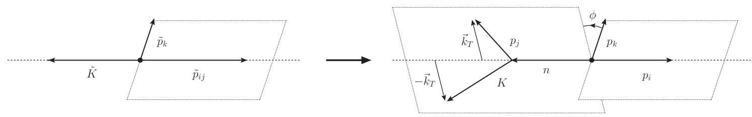
We will first describe the kinematics mapping needed for soft evolution. This is sketched in Fig. 1. The momenta and are mapped to the momenta , and , while acts as a spectator that defines the azimuthal direction. We assume that any of the particles , and can be massive. The momentum can be chosen in a suitable way to reflect the dynamics of the process Herren et al. (2022) and absorbs the recoil in the splitting. We define the variables
| (13) |
and the analogous final-state variables
and
.
The scalar invariants after the splitting are defined in terms of
the energy fraction, Catani and Seymour (1997)
| (14) |
The momentum of the radiator after the emission is
| (15) |
where
| (16) |
We define the variable
| (17) |
and where is defined as in the massless case Catani and Seymour (1997); Herren et al. (2022). In terms of these quantities, the gluon momentum is given by
| (18) |
where
| (19) |
In order to determine a reference direction for the azimuthal angle , we note that the soft radiation pattern must be correctly generated. To achieve this, we compose the transverse momentum as
| (20) |
where the reference axes and are given by the transverse projections222In kinematical configurations where is a linear combination of and , in the definition of Eq. (20) vanishes. It can then be computed using , where may be any index that yields a nonzero result. Note that in this case, the matrix element cannot depend on the azimuthal angle.
| (21) |
and
| (22) |
Since the differential emission phase-space element is a Lorentz-invariant quantity, the azimuthal angle is Lorentz invariant Herren et al. (2022). This allows us to write the emission phase-space in a frame-independent way. Upon construction of the momenta , and , the momenta which are used to define are subjected to a Lorentz transformation,
| (23) |
III.2 Splitting kinematics
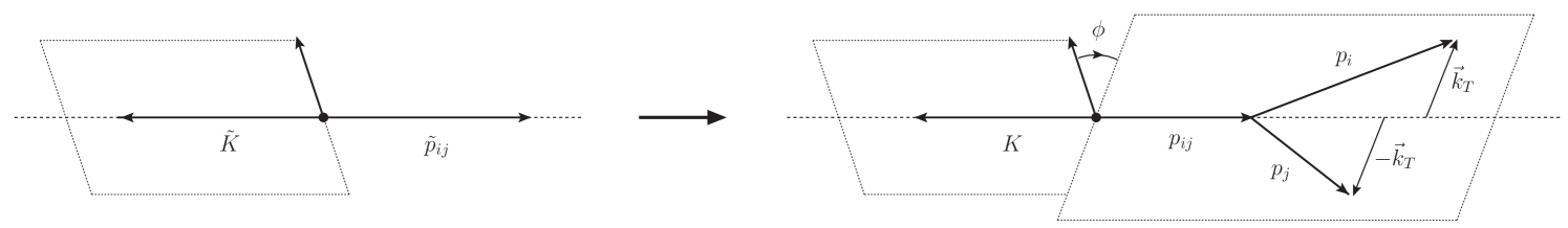
In this section, we describe the kinematics for the implementation of the purely collinear components of the splitting functions in Eq. (12). This is sketched in Fig. 2. We make use of some of the notation in Catani et al. (2002), in particular
| (24) |
and we define the scaled masses
| (25) |
We also introduce the following variables
| (26) |
In terms of the additional variables
| (27) |
the momenta after the splitting are given by
| (28) |
The transverse momentum squared is given by
| (29) |
The construction of the transverse momentum vector proceeds as described in Sec. III.1. While the choice of the reference vector defining is in principle arbitrary, it can be made conveniently, e.g., to aid the implementation of spin correlations in collinear gluon splittings.
IV Phase space factorization
In this section, we discuss the factorization of the differential particle phase-space element into a differential particle phase-space element and the radiative phase space. We start from the generic four-dimensional expression for the initial-state momenta and and final-state momenta, ,
| (30) |
Replacing particles and with a combined “mother” particle , we can write the expression for the underlying Born phase space as
| (31) |
The ratio of differential phase-space elements after and before the mapping is defined as the differential phase-space element for the one-particle emission process
| (32) |
This expression naturally generalizes to dimensions. It can be computed using the lowest final-state multiplicity, i.e., . In order to do so, we first derive a suitable expression for the -dimensional two-particle phase space in the frame of an arbitrary, time-like momentum . It reads
| (33) |
where is the integral over the dimensional solid angle of in the frame of . All energies and momenta are computed in this frame, and we have defined . We can re-write the momentum-dependent denominator factor on the right-hand side of Eq. (33) as
| (34) |
Inserting this into Eq. (33), and using , we obtain a manifestly covariant form of the phase-space element,
| (35) |
IV.1 Radiation kinematics
To derive the emission phase space for final-state splittings in the radiation kinematics of Sec. III.1, we make use of the standard factorization formula
| (36) |
where is the sum of all final-state momenta except and . We can use Eq. (35) to relate the phase-space factor to the underlying Born phase space as follows
| (37) |
where we have defined
| (38) |
The differential two-body phase-space element for the production of and is given by
| (39) |
Finally, we combine Eqs. (37) and (39) to obtain the single-emission phase space element in Eq. (32)
| (40) |
In the massless limit, this simplifies to
| (41) |
We demonstrate in App. A.1 that this expression agrees with the result derived in Ref. Catani and Seymour (1997).
IV.2 Splitting kinematics
To derive the emission phase space for final-state radiation in the splitting kinematics of Sec. III.2, the recoiler is chosen to be the sum of the remaining final-state partons. We make use of the standard factorization formula
| (42) |
where is the sum of final-state momenta except and . Working in the frame of , we can use Eq. (35) to relate the phase-space factor to the underlying Born differential phase space element as follows
| (43) |
The decay of the intermediate off-shell parton is associated with the differential phase-space element
| (44) |
Finally, we combine Eqs. (43) and (44) to obtain
| (45) |
In the massless limit, this simplifies to
| (46) |
In App. A.2, we will show the equivalence of Eq. (45) to the single-emission differential phase-space element of Catani et al. (2002).
V Infrared subtraction terms at next-to-leading order
The matching of parton showers to fixed-order NLO calculations in dimensional regularization based on the MC@NLO algorithm Frixione and Webber (2002) requires the knowledge of integrated splitting functions in dimensions. Since our technique for massive parton evolution is modeled on the Catani-Seymour identified particle subtraction and the Alaric parton-shower, we can use the methods developed in Höche et al. (2019); Liebschner (2020). We will limit the discussion to the main changes needed to implement the algorithm for massive partons. The results of this section provide an extension of the subtraction method for identified hadrons first introduced in Catani and Seymour (1997).
V.1 Soft angular integrals
In this section, we compute the angular integrals of the partial fractioned soft eikonal. While we focus on pure final-state radiation, the results of this integration are generic and apply to the case of final-state and initial-state emission of massless vector bosons. The integrand is given by Eq. (8),
| (47) |
We can write the angular phase space for the emission of the massless particle as
| (48) |
where is the -dimensional line element, in particular . We finally find the following expression for the cases with massive emitter
| (49) |
For massless emitter, we obtain (see also Catani and Seymour (1997); Herren et al. (2022))
| (50) |
The angular integrals and have been computed in van Neerven (1986); Beenakker et al. (1989); Somogyi (2011); Isidori et al. (2020); Lyubovitskij et al. (2021). They read Lyubovitskij et al. (2021)
| (51) |
where the velocities are defined in the notation of Ref. Lyubovitskij et al. (2021), and where
| (52) |
Note that spurious collinear poles appear on the right-hand side of Eq. (50), which cancel between and . In addition, in the fully massless case is related to the massless two-denominator integral and gives the simple result Herren et al. (2022)
| (53) |
V.2 Soft energy integrals
In this section, we introduce the basic techniques to solve the energy integrals in Eq. (40). After performing the angular integrals, we are left with the additional -dependence induced by the energy denominator in Eq. (4). We focus on the cases relevant for QCD and QED soft radiation, where and . The differential emission probability per dipole is then given by
| (54) |
In order to carry out the integration over the energy fraction, , we expand the integrand into a Laurent series. The differential soft subtraction counterterm, summed over all dipoles, is given by
| (55) |
where , and where the mass correction factor reads
| (56) |
and where the massless limit is given by . All poles have been extracted, and we can (after expanding the -dependent prefactors) compute the final result as an integral over the delta functions and plus distributions in . In general, some of the terms must be computed numerically, as implicitly depends on , see Eq. (14). In order to apply Eq. (56) to processes with resolved hadrons, we can make use of the formalism derived in Catani and Seymour (1997); Höche et al. (2019); Liebschner (2020). The pole proportional to can then be combined with the soft enhanced part of the collinear mass factorization counterterms. The extension to initial-state radiation requires a repetition of the derivation in Sec. IV.1 for initial-state kinematics. We will discuss this in a future publication.
V.3 Collinear integrals
To compute the purely collinear counterterms, we use the splitting kinematics and make use of the results in App. A.2. Note that we also use the corresponding definitions of the scaled masses. We define the purely collinear anomalous dimension in terms of the collinear remainders in Eq. (12)
| (57) |
where are given by Eq. (77). This leads to
| (58) |
The complete counterterm can now be obtained by Laurent series expansion, using Eq. (82)
| (59) |
There are three variants of Eq. (59) relevant for QCD. The first describes the collinear splitting of a massive quark into a quark and a gluon, and is characterized by and . We obtain
| (60) |
Note that the result is infrared finite. This is expected because the only poles that occur in the radiation off massive quarks have their origin in soft gluon emission, which is fully accounted for by the eikonal integral in Eq. (54). This also shows that in our subtraction scheme, there is a hierarchy between the soft and the collinear enhancements, as required for a proper classification of leading and sub-leading logarithms.
The second case is the splitting of a gluon into two massive quarks, which is characterized by and . The result is finite and reads
| (61) |
The final case describes the collinear decay of a massless parton into two massless partons, and is characterized by . This term is collinearly divergent, and we obtain
| (62) |
The treatment of initial-state singularities will be discussed in a future publication.
VI Kinematical effects on sub-leading logarithmic corrections
We now demonstrate that our kinematics mapping satisfies the criteria for NLL accuracy laid out in Dasgupta et al. (2018, 2020), extending the discussion of the massless case in Herren et al. (2022). We refer the reader to Herren et al. (2022) for more details on the general method of the proof. The analysis is based on the technique for general final-state resummation introduced in Banfi et al. (2005). Following the notation of Sec. 2 of Banfi et al. (2005), the observable to be resummed is denoted by , while the hard partons and soft emission have momenta and , respectively. The observable is a function of these momenta, , and for any radiating color dipole formed by the hard momenta, and , the momentum of a single emission can be parametrized as
| (63) |
with rapidity . An observable can be expressed as
| (64) |
with and for in the collinear limit. A natural extension of Eq. (63) to the case of massive emitters would be
| (65) |
In the quasi-collinear limit, this Sudakov decomposition agrees with the one given in Catani et al. (2001); Cacciari and Catani (2001) if the auxiliary (light-like) vector defining the anti-collinear direction is chosen as the direction of the color partner of the QCD dipole. In particular, for constant , and small , the gluon momentum behaves as
| (66) |
in complete agreement with Eq. (63). In the quasi-collinear limit, the value of the observable will therefore be unchanged from the case of massless evolution. However, both the Sudakov radiator and the function will change, due to the modified splitting functions, Eq. (10), and the effects of masses on the integration boundaries.
The Lund plane for gluon emission off a dipole containing a massive quark with mass and energy will have a smooth upper rapidity bound at , consistent with the well known dead-cone effect Marchesini and Webber (1990); Dokshitzer et al. (1991); Ghira et al. (2023). When the similarity transformation introduced in Sec. 2.2.3 of Banfi et al. (2005) is generalized to the quasi-collinear limit, and applied to a process with massive quarks, the location of this boundary in relative rapidity is unchanged, because the quasi-collinear limit requires . The sub-leading logarithmic terms in the resummed cross section can then be extracted similarly to the massless case, but a change to the CMW scheme is required. We will not discuss the complete structure of the result, but address only the effects related to momentum mapping, which have been found to spoil NLL precision Dasgupta et al. (2018, 2020).
In order to prove that the momentum mapping of Sec. III.1 satisfies the criteria laid out in Dasgupta et al. (2018, 2020), we need to show that it has the same topological features as in the massless case Herren et al. (2022). This amounts to showing that hard, (quasi-)collinear emissions, i.e. highly energetic emissions in the direction of the hard partons, do not generate Lorentz transformations that change existing momenta by more than , where is a positive exponent. To show this, we analyze the behavior of Eq. (23) in the (quasi-)collinear region. We can split into its components along the original recoil momentum, , the emitter, , and the emission, .
| (67) |
For the effect of the Lorentz transformation that determines the event topology after radiation, only the parametric form of is of interest. Using Eqs. (15) and (18), the small momentum for gluon radiation can be written as
| (68) |
In the quasi-collinear limit, this scales as , which is sufficient to make the effect of the Lorentz transformation vanish even for hard quasi-collinear splittings.
Finally, we note that the precise treatment of transverse recoil in the kinematics mapping of Sec. III.2 does not affect the resummed result at NLL precision, because the mapping is applied solely to the purely collinear parts of the splitting functions, Eq. (12). This can be understood with the help of Eq. (2.46) in Ref. Banfi et al. (2005), which will be structurally similar in the case of massive partons. The sub-leading logarithmic terms, which lead to a violation of NLL accuracy in many dipole showers, arise from accidental correlations between multiple soft-enhanced emissions. This means in particular, that the parton-shower equivalent of the integrals in Eq. (2.46) does not factorize in the strongly ordered limit. The differential probability for the emissions is given by the derivative of the radiator function in Eq. (2.21) of Ref. Banfi et al. (2005) and does not receive a contribution from the purely collinear remainders in Eq. (12), such that a change in the kinematics mapping cannot generate this particular type of NLL violation.
VII Comparison to experimental data
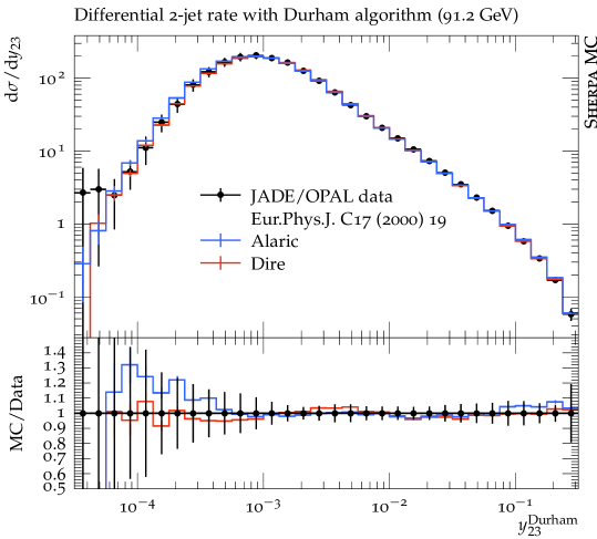
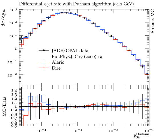
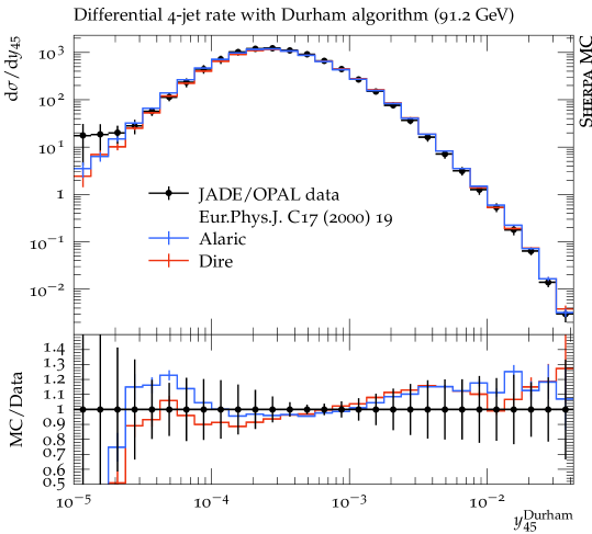
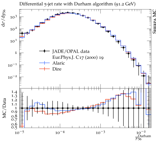
In this section we present first numerical results obtained with the extension of the Alaric final-state parton shower to massive parton evolution. The implementation is part of the event generation framework Sherpa Gleisberg et al. (2004, 2009); Bothmann et al. (2019). We do not perform NLO matching or multi-jet merging, and we set and . The quark masses are set to GeV and GeV and the same flavor thresholds are used for the evaluation of the strong coupling. The running coupling is evaluated at two loop accuracy, and we set . Following standard practice to improve the logarithmic accuracy of the parton shower, we employ the CMW scheme Catani et al. (1991). In this scheme, the soft eikonal contribution to the flavor conserving splitting functions is rescaled by , where , and where is scale dependent with the same flavor thresholds as listed above. Velocity dependent corrections to should be included in principle, but the massless result provides an acceptable approximation at very large velocities Korchemsky and Radyushkin (1987); Kidonakis (2009), and can therefore be used for -quark production at LEP, where . Our results include the simulation of hadronization using the Lund string fragmentation implemented in Pythia 6.4 Sjöstrand et al. (2006). We use the default hadronization parameters, apart from the following: PARJ(21)=0.3, PARJ(41)=0.4, PARJ(42)=0.45, PARJ(46)=0.5 and compare our predictions with those from the Dire parton shower Höche and Prestel (2015). All analyses are performed with Rivet Buckley et al. (2013).
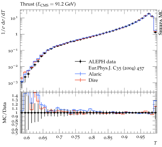
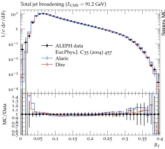
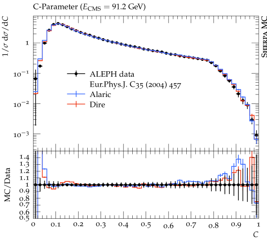
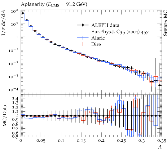
Figure 3 displays predictions from the Alaric parton shower for differential jet rates in the Durham scheme compared to experimental results from the JADE and OPAL collaborations Pfeifenschneider et al. (2000). The -quark mass corresponds to , and hadronization effects dominate the predictions below . We observe good agreement with the experimental data. Overall, the quality of the results is similar to Ref. Herren et al. (2022), where heavy quark effects were modeled by thresholds. Figure 4 shows a comparison for event shapes measured by the ALEPH collaboration Heister et al. (2004). It can be expected that the numerical predictions will improve upon including matrix-element corrections, or when merging the parton shower with higher-multiplicity calculations. Again, the overall quality of the prediction is similar to Ref. Herren et al. (2022).
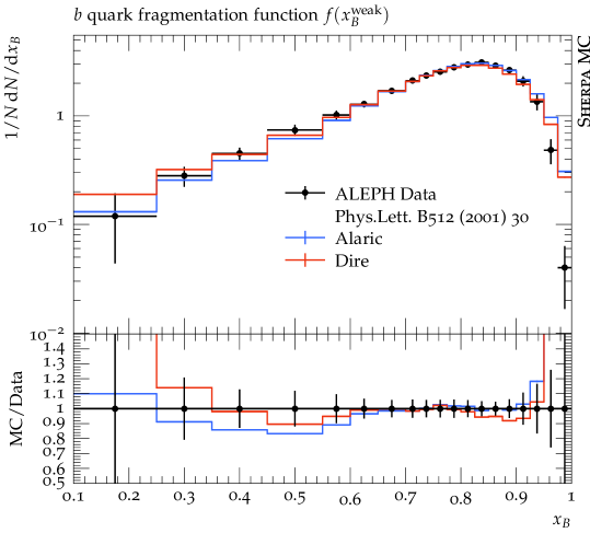
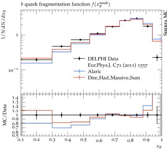
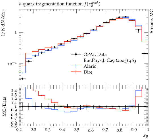
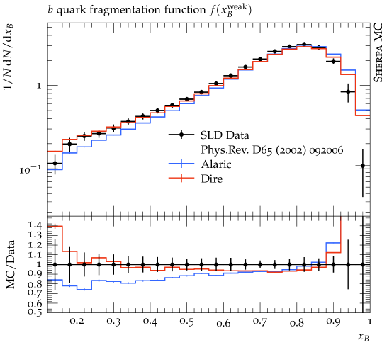
Finally, we show predictions for the -quark fragmentation function as measured by the ALEPH Heister et al. (2001), DELPHI Abdallah et al. (2011), OPAL Abbiendi et al. (2003) and SLD Abe et al. (2002) collaborations. Figure 5 shows a fair agreement of both the Alaric and Dire predictions with experimental data. We note that both parton shower implementations use the same hadronization tune.
VIII Conclusions
We have introduced an extension of the recently proposed Alaric parton-shower model to the case of massive QCD evolution. An essential aspect of the new algorithm is the form of the collinearly matched massive eikonal, which is obtained by partial fractioning the angular component of the eikonal of a complete dipole. This technique preserves the positivity of the splitting function, thus leading to an excellent efficiency of the Monte-Carlo simulation. Inspired by the symmetry of the partonic final state in purely collinear splittings, we also introduced a dedicated kinematics mapping for this scenario and showed that it preserves the NLL precision of the overall simulation. We computed the infrared counterterms needed for the matching to fixed-order calculations at NLO accuracy, and discussed the logarithmic structure of the resummation in the case of heavy-quark evolution.
Several improvements of this algorithm are needed before it can be considered on par with the parton shower simulations used by past and current experiments. Clearly, spin correlations and dominant sub-leading color effects should be included. This can be achieved with the help of the techniques from Collins (1988); Knowles (1988a, b, 1990); Gustafson (1993); Dulat et al. (2018); Hamilton et al. (2021). An extension to initial-state evolution is needed for LHC phenomenology. It will need to account for the non-cancellation of certain types of singularities in processes with two massive initial states Caola et al. (2021). Finally, the algorithm should be extended to higher orders based on the techniques developed in Höche and Prestel (2017); Dulat et al. (2018); Gellersen et al. (2022).
In this context, we note that the all-orders (in ) expressions from Sec. V, in conjunction with higher-order expressions for the angular integrals in Sec. V.1 that can be obtained from Lyubovitskij et al. (2021), can be used to compute the factorizable integrals at NNLO, thus providing a significant part of the components needed for an MC@NNLO matching Campbell et al. (2023). The computation of the remaining non-factorizable integrals is a further development needed in order to reach the precision targets of the high-luminosity LHC.
Acknowledgments
We thank John Campbell, Florian Herren and Simone Marzani for many helpful and inspiring discussions. We are grateful to Davide Napoletano and Pavel Nadolsky for clarifying various questions on PDFs and the implementation of the FONLL and ACOT schemes. This work was supported by the Fermi National Accelerator Laboratory (Fermilab), a U.S. Department of Energy, Office of Science, HEP User Facility. Fermilab is managed by Fermi Research Alliance, LLC (FRA), acting under Contract No. DE–AC02–07CH11359.
Appendix A Phase-space factorization in comparison to other infrared subtraction schemes
In this appendix, we compare the phase-space factorization in our method to the existing dipole subtraction schemes of Refs. Catani and Seymour (1997) and Catani et al. (2002). We will show that our generic form of the factorized phase space, derived from Eq. (35) can be used to obtain the relevant formulae, for pure final-state evolution.
A.1 Massless radiation kinematics
First, we show that Eq. (5.189) of Ref. Catani and Seymour (1997) can be derived from our generic expression, Eq. (35), using radiation kinematics. We start with the massless limit of Eq. (40)
| (69) |
Expressing the polar angle in the frame of in terms of and (see also Eq. (32) of Herren et al. (2022))
| (70) |
we can perform a change of integration variables , leading to Eq. (5.189) of Ref. Catani and Seymour (1997).
| (71) |
A.2 Massive splitting kinematics
In this appendix, we derive the phase-space factorization formula, Eq. (5.11) in Catani et al. (2002) from our generic expression, Eq. (35). We use the definitions of Eq. (24) Catani et al. (2002), and we set . In addition, we define the scaled masses333 Note that these definitions differ from the ones in Sec. III.2.
| (72) |
The single-emission phase space element is given by
| (73) |
The decay of is simplest to compute in its rest frame. In this frame, we can write
| (74) |
where the velocities are given by
| (75) |
The decay phase space, written in the frame of , then reads
| (76) |
We can use the factorization Ansatz , where the physical boundary condition gives the roots of the quadratic , leading to
| (77) |
The factor is determined by equating the transverse momentum at the extremal point to the total three-momentum of in the frame of . This leads to
| (78) |
and finally
| (79) |
We also have
| (80) |
The last missing component of the emission phase space is the ratio of the production to the underlying Born phase-space element. It is most easily computed in the frame of and results in
| (81) |
where the Källen function is given by . Combining Eqs. (79)-(81) gives the final result
| (82) |
References
- Mangano et al. (1992) M. L. Mangano, P. Nason, and G. Ridolfi, Nucl. Phys. B 373, 295 (1992).
- Bonciani et al. (1998) R. Bonciani, S. Catani, M. L. Mangano, and P. Nason, Nucl. Phys. B 529, 424 (1998), [Erratum: Nucl.Phys.B 803, 234 (2008)], hep-ph/9801375 .
- Cacciari et al. (2004) M. Cacciari, S. Frixione, M. L. Mangano, P. Nason, and G. Ridolfi, JHEP 07, 033 (2004), hep-ph/0312132 .
- Cacciari et al. (2012) M. Cacciari, S. Frixione, N. Houdeau, M. L. Mangano, P. Nason, and G. Ridolfi, JHEP 10, 137 (2012), arXiv:1205.6344 [hep-ph] .
- Norrbin and Sjöstrand (2001) E. Norrbin and T. Sjöstrand, Nucl. Phys. B 603, 297 (2001), hep-ph/0010012 .
- Gieseke et al. (2003) S. Gieseke, P. Stephens, and B. Webber, JHEP 12, 045 (2003), hep-ph/0310083 .
- Schumann and Krauss (2008) S. Schumann and F. Krauss, JHEP 03, 038 (2008).
- Gehrmann-De Ridder et al. (2012) A. Gehrmann-De Ridder, M. Ritzmann, and P. Z. Skands, Phys. Rev. D 85, 014013 (2012), arXiv:1108.6172 [hep-ph] .
- Krauss and Napoletano (2018) F. Krauss and D. Napoletano, Phys. Rev. D 98, 096002 (2018), arXiv:1712.06832 [hep-ph] .
- Herren et al. (2022) F. Herren, S. Höche, F. Krauss, D. Reichelt, and M. Schönherr, (2022), arXiv:2208.06057 [hep-ph] .
- Catani et al. (2002) S. Catani, S. Dittmaier, M. H. Seymour, and Z. Trocsanyi, Nucl. Phys. B 627, 189 (2002), hep-ph/0201036 .
- Mangano et al. (2002) M. L. Mangano, M. Moretti, and R. Pittau, Nucl. Phys. B 632, 343 (2002), hep-ph/0108069 .
- Frixione et al. (2003) S. Frixione, P. Nason, and B. R. Webber, JHEP 08, 007 (2003), hep-ph/0305252 .
- Frixione et al. (2007) S. Frixione, P. Nason, and G. Ridolfi, JHEP 09, 126 (2007), arXiv:0707.3088 [hep-ph] .
- Höche et al. (2013) S. Höche, J. Huang, G. Luisoni, M. Schönherr, and J. Winter, Phys. Rev. D 88, 014040 (2013), arXiv:1306.2703 [hep-ph] .
- Lyubovitskij et al. (2021) V. E. Lyubovitskij, F. Wunder, and A. S. Zhevlakov, JHEP 06, 066 (2021), arXiv:2102.08943 [hep-ph] .
- Dokshitzer (1977) Y. L. Dokshitzer, Sov. Phys. JETP 46, 641 (1977).
- Gribov and Lipatov (1972) V. N. Gribov and L. N. Lipatov, Sov. J. Nucl. Phys. 15, 438 (1972).
- Lipatov (1975) L. N. Lipatov, Sov. J. Nucl. Phys. 20, 94 (1975).
- Altarelli and Parisi (1977) G. Altarelli and G. Parisi, Nucl. Phys. B126, 298 (1977).
- Catani et al. (2001) S. Catani, S. Dittmaier, and Z. Trocsanyi, Phys. Lett. B 500, 149 (2001), hep-ph/0011222 .
- Bassetto et al. (1983) A. Bassetto, M. Ciafaloni, and G. Marchesini, Phys. Rept. 100, 201 (1983).
- Catani and Seymour (1997) S. Catani and M. H. Seymour, Nucl. Phys. B 485, 291 (1997), [Erratum: Nucl.Phys.B 510, 503–504 (1998)], hep-ph/9605323 .
- Webber (1986) B. Webber, Ann. Rev. Nucl. Part. Sci. 36, 253 (1986).
- Höche and Prestel (2015) S. Höche and S. Prestel, Eur. Phys. J. C 75, 461 (2015), arXiv:1506.05057 [hep-ph] .
- Dasgupta et al. (2018) M. Dasgupta, F. A. Dreyer, K. Hamilton, P. F. Monni, and G. P. Salam, JHEP 09, 033 (2018), [Erratum: JHEP 03, 083 (2020)].
- Dasgupta et al. (2020) M. Dasgupta, F. A. Dreyer, K. Hamilton, P. F. Monni, G. P. Salam, and G. Soyez, Phys. Rev. Lett. 125, 052002 (2020).
- Frixione and Webber (2002) S. Frixione and B. R. Webber, JHEP 06, 029 (2002).
- Höche et al. (2019) S. Höche, S. Liebschner, and F. Siegert, Eur. Phys. J. C 79, 728 (2019).
- Liebschner (2020) S. Liebschner, PhD thesis, (2020), CERN-THESIS-2020-126.
- van Neerven (1986) W. L. van Neerven, Nucl. Phys. B 268, 453 (1986).
- Beenakker et al. (1989) W. Beenakker, H. Kuijf, W. L. van Neerven, and J. Smith, Phys. Rev. D 40, 54 (1989).
- Somogyi (2011) G. Somogyi, J. Math. Phys. 52, 083501 (2011), arXiv:1101.3557 [hep-ph] .
- Isidori et al. (2020) G. Isidori, S. Nabeebaccus, and R. Zwicky, JHEP 12, 104 (2020), arXiv:2009.00929 [hep-ph] .
- Banfi et al. (2005) A. Banfi, G. P. Salam, and G. Zanderighi, JHEP 03, 073 (2005).
- Cacciari and Catani (2001) M. Cacciari and S. Catani, Nucl. Phys. B 617, 253 (2001), hep-ph/0107138 .
- Marchesini and Webber (1990) G. Marchesini and B. R. Webber, Nucl. Phys. B 330, 261 (1990).
- Dokshitzer et al. (1991) Y. L. Dokshitzer, V. A. Khoze, and S. I. Troian, J. Phys. G 17, 1602 (1991).
- Ghira et al. (2023) A. Ghira, S. Marzani, and G. Ridolfi, (2023), arXiv:2309.06139 [hep-ph] .
- Pfeifenschneider et al. (2000) P. Pfeifenschneider et al., Eur. Phys. J. C17, 19 (2000).
- Heister et al. (2004) A. Heister et al., Eur. Phys. J. C35, 457 (2004).
- Heister et al. (2001) A. Heister et al. (ALEPH), Phys. Lett. B 512, 30 (2001), hep-ex/0106051 .
- Abdallah et al. (2011) J. Abdallah et al. (DELPHI), Eur. Phys. J. C 71, 1557 (2011), arXiv:1102.4748 [hep-ex] .
- Abbiendi et al. (2003) G. Abbiendi et al. (OPAL), Eur. Phys. J. C 29, 463 (2003), hep-ex/0210031 .
- Abe et al. (2002) K. Abe et al. (SLD), Phys. Rev. D 65, 092006 (2002), [Erratum: Phys.Rev.D 66, 079905 (2002)], hep-ex/0202031 .
- Gleisberg et al. (2004) T. Gleisberg, S. Höche, F. Krauss, A. Schälicke, S. Schumann, and J. Winter, JHEP 02, 056 (2004).
- Gleisberg et al. (2009) T. Gleisberg, S. Höche, F. Krauss, M. Schönherr, S. Schumann, F. Siegert, and J. Winter, JHEP 02, 007 (2009).
- Bothmann et al. (2019) E. Bothmann et al., SciPost Phys. 7, 034 (2019).
- Catani et al. (1991) S. Catani, B. R. Webber, and G. Marchesini, Nucl. Phys. B349, 635 (1991).
- Korchemsky and Radyushkin (1987) G. P. Korchemsky and A. V. Radyushkin, Nucl. Phys. B 283, 342 (1987).
- Kidonakis (2009) N. Kidonakis, Phys. Rev. Lett. 102, 232003 (2009), arXiv:0903.2561 [hep-ph] .
- Sjöstrand et al. (2006) T. Sjöstrand, S. Mrenna, and P. Skands, JHEP 05, 026 (2006).
- Buckley et al. (2013) A. Buckley et al., Comput.Phys.Commun. 184, 2803 (2013).
- Collins (1988) J. C. Collins, Nucl.Phys. B304, 794 (1988).
- Knowles (1988a) I. Knowles, Nucl.Phys. B304, 767 (1988a).
- Knowles (1988b) I. Knowles, Nucl.Phys. B310, 571 (1988b).
- Knowles (1990) I. Knowles, Comput.Phys.Commun. 58, 271 (1990).
- Gustafson (1993) G. Gustafson, Nucl. Phys. B 392, 251 (1993).
- Dulat et al. (2018) F. Dulat, S. Höche, and S. Prestel, Phys. Rev. D98, 074013 (2018).
- Hamilton et al. (2021) K. Hamilton, R. Medves, G. P. Salam, L. Scyboz, and G. Soyez, JHEP 03, 041 (2021).
- Caola et al. (2021) F. Caola, K. Melnikov, D. Napoletano, and L. Tancredi, Phys. Rev. D 103, 054013 (2021), arXiv:2011.04701 [hep-ph] .
- Höche and Prestel (2017) S. Höche and S. Prestel, Phys. Rev. D96, 074017 (2017).
- Gellersen et al. (2022) L. Gellersen, S. Höche, and S. Prestel, Phys. Rev. D 105, 114012 (2022).
- Campbell et al. (2023) J. M. Campbell, S. Höche, H. T. Li, C. T. Preuss, and P. Skands, Phys. Lett. B 836, 137614 (2023), arXiv:2108.07133 [hep-ph] .