A new class of discrete conformal structures on surfaces with boundary

Xu Xu

Abstract

We introduce a new class of discrete conformal structures on surfaces with boundary, which have nice interpolations in 3-dimensional hyperbolic geometry. Then we prove the global rigidity of the new discrete conformal structures using variational principles, which is a complement of Guo-Luo’s rigidity of the discrete conformal structures in [14] and Guo’s rigidity of vertex scaling in [13] on surface with boundary. As a result, new convexities of the volume of generalized hyperbolic pyramids with right-angled hyperbolic hexagonal bases are obtained. Motivated by Chow-Luo’s combinatorial Ricci flow and Luo’s combinatorial Yamabe flow on closed surfaces, we further introduce combinatorial Ricci flow and combinatorial Calabi flows to deform the new discrete conformal structures on surfaces with boundary. The basic properties of these combinatorial curvature flows are established. These combinatorial curvature flows provide effective algorithms for constructing hyperbolic metrics on surfaces with totally geodesic boundary components of prescribed lengths.

MSC (2020): 52C26

Keywords: Rigidity; Discrete conformality; Combinatorial Ricci flow; Surfaces with boundary; Hyperbolic geometry

1 Introduction

Discrete conformal structure on polyhedral manifolds is a discrete analogue of the well-known conformal structure on smooth Riemannian manifolds, which assigns the discrete metrics defined on the edges by scalar functions defined on the vertices. Since the famous work of William Thurston on circle packings on closed surfaces [28], different types of discrete conformal structures on closed surfaces has been extensively studied. See, for instance, [1, 2, 28, 9, 10, 11, 12, 16, 18, 19, 8, 26, 29, 30, 32, 33, 15, 25] and others.

However, the discrete conformal structures on surfaces with boundary are seldom studied. Motivated by Thurston’s circle packings on closed surfaces, Guo-Luo [14] first introduced some generalized circle packing type hyperbolic discrete conformal structures on surfaces with boundary. Following Luo’s vertex scaling of piecewise linear metrics on closed surfaces [16], Guo [13] introduced a class of hyperbolic discrete conformal structures, also called vertex scaling, on surfaces with boundary. In this paper, we introduce a new class of hyperbolic discrete conformal structures on ideally triangulated surfaces with boundary, which has nice geometric interpolations in 3-dimensional hyperbolic geometry. Then we study the rigidity and deformation of the new discrete conformal structures on surfaces with boundary.

Suppose $\Sigma$ is a compact surface with boundary $B$ , which is composed of $n$ boundary components. $\mathcal{T}$ is an ideal triangulation of $\Sigma$ , which can be constructed as follows. Suppose we have a finite disjoint union of colored topological hexagons, three non-adjacent edges of each hexagon are colored red and the other edges are colored black. Please refer to Figure 1 for a colored hexagon. Identifying the red edges of colored hexagons in pairs by homeomorphisms gives rise to a quotient space, called an ideal triangulated compact surface with boundary. The image of each colored hexagon is a face in the triangulation $\mathcal{T}$ and the image of each red edge in the colored hexagon is an edge in the triangulation $\mathcal{T}$ . The image of the black edges are referred as boundary arcs. For simplicity, we denote the boundary components of $(\Sigma,\mathcal{T})$ as $B=\{1,2,\cdots,n\}$ , denote the set of edges in $(\Sigma,\mathcal{T})$ as $E$ and denote the set of faces in $(\Sigma,\mathcal{T})$ as $F$ . An edge connecting the boundary components $i,j\in B$ is denoted by $\{ij\}$ and a face adjacent to $i,j,k\in B$ is denoted by $\{ijk\}$ .

A basic fact from hyperbolic geometry [22] is that given any three positive numbers, there exists a unique right-angled hyperbolic hexagon up to hyperbolic isometry with the lengths of three non-adjacent edges in the hexagon given by the three positive numbers. Therefore, if $l:E\rightarrow(0,+\infty)$ is a positive function defined on $E$ , every face in $F$ can be realized as a unique right-angled hyperbolic hexagon up to isometry with the lengths of edges in $E$ given by $l$ . By gluing the right-angled hyperbolic hexagons along the edges in $E$ in pairs by isomorphisms according to the ideal triangulation $\mathcal{T}$ , we get a hyperbolic metric on the ideally triangulated surface $(\Sigma,\mathcal{T})$ with totally geodesic boundary components. Conversely, every hyperbolic metric on an ideally triangulated surface $(\Sigma,\mathcal{T})$ with totally geodesic boundary components with $\mathcal{T}$ geometric determines a unique map $l:E\rightarrow(0,+\infty)$ with $l_{ij}$ given by the length of the shortest geodesic connecting the boundary components $i,j\in B$ . The map $l:E\rightarrow(0,+\infty)$ is called as a discrete hyperbolic metric on $(\Sigma,\mathcal{T})$ . The length $K_{i}$ of the boundary component $i\in B$ is called the generalized combinatorial curvature of the discrete hyperbolic metric $l:E\rightarrow(0,+\infty)$ at $i\in B$ .

Refer to caption — Figure 1: Colored right-angled hyperbolic hexagon

Note that every colored right-angled hyperbolic hexagon in the hyperbolic space corresponds to a unique generalized hyperbolic triangle in the extended hyperbolic space (using the Klein model) with three hyper-ideal vertices and the three segments between the hyper-ideal vertices intersecting with the hyperbolic plane $\mathbb{H}^{2}$ . Please refer to Figure 1. Further note that for the colored right-angled hyperbolic hexagons adjacent to the same boundary components, the corresponding generalized triangles are adjacent to same hyper-ideal vertex. In this sense, the ideally triangulated hyperbolic surface with boundary $(\Sigma,\mathcal{T},l)$ can be taken as a triangulated closed surface in the extended hyperbolic space, with the totally geodesic boundary components corresponding to the hyper-ideal vertices. For simplicity, a generalized hyperbolic triangle is always referred to a right-angled hyperbolic hexagon in the following, if it causes no confusion in the context. Recall that a discrete conformal structure on a triangulated closed surface assigns the discrete metrics defined on the edges by functions defined on the vertices. Motivated by the following hyperbolic discrete conformal structures introduced by Glickenstein-Thomas [8], Zhang-Guo-Zeng-Luo-Yau-Gu [38] and Bobenko-Pinkall-Springborn [1] on triangulated closed surfaces

\displaystyle l_{ij}=\cosh^{-1}\left(\sqrt{(1+\varepsilon_{i}e^{2u_{i}})(1+\varepsilon_{j}e^{2u_{j}})}+\eta_{ij}e^{u_{i}+u_{j}}\right)

with $\varepsilon_{i},\varepsilon_{j}\in\{-1,0,1\}$ and $\eta_{ij}\in\mathbb{R}$ , we introduce the following discrete conformal structures on ideally triangulated surfaces with boundary.

Definition 1.

Suppose $(\Sigma,\mathcal{T})$ is an ideally triangulated surface with boundary and $\eta:E\rightarrow(-1,+\infty)$ is a weight defined on the edges. A discrete conformal structure on $(\Sigma,\mathcal{T})$ is a function $u:B\rightarrow\mathbb{R}$ such that

\displaystyle l_{ij}=\cosh^{-1}\left(e^{u_{i}+u_{j}}+\eta_{ij}\sqrt{(1+e^{2u_{i}})(1+e^{2u_{j}})}\right)

(1.1)

determines a discrete hyperbolic metric $l:E\rightarrow(0,+\infty)$ on $(\Sigma,\mathcal{T})$ . The function $u:B\rightarrow\mathbb{R}$ is called a discrete conformal factor.

A basic problem in discrete conformal geometry is to understand the relationships between the discrete conformal structures and their combinatorial curvatures. We prove the following result on the rigidity of the discrete conformal structures in Definition 1.

Theorem 1.1.

Suppose $(\Sigma,\mathcal{T})$ is an ideally triangulated surface with boundary and $\eta:E\rightarrow(-1,+\infty)$ is a weight defined on the edges. If the weight $\eta$ satisfies the following structure condition

\displaystyle\eta_{ij}+\eta_{ik}\eta_{jk}\geq 0,\eta_{ik}+\eta_{ij}\eta_{jk}\geq 0,\eta_{jk}+\eta_{ij}\eta_{ik}\geq 0

(1.2)

for any face $\{ijk\}\in F$ , then the generalized combinatorial curvature $K:B\rightarrow(0,+\infty)$ uniquely determines the discrete conformal factor $u:B\rightarrow\mathbb{R}$ .

Remark 1.

The structure condition (1.2) is a direct consequence of the cosine law for generalized hyperbolic triangles with all vertices hyper-ideal. Please refer to Section 5.1 in [35] and Remark 8 in Section 6 of this paper for the details of the geometric explanation. The structure condition (1.2) has been previously used in the study of discrete conformal structures on closed surfaces. See, for instance, [39, 33, 34, 35] and others. The rigidity result in Theorem 1.1 can be taken to be a complement of Guo-Luo’s rigidity of the discrete conformal structures in [14] and Guo’s rigidity of vertex scaling in [13] on surface with boundary.

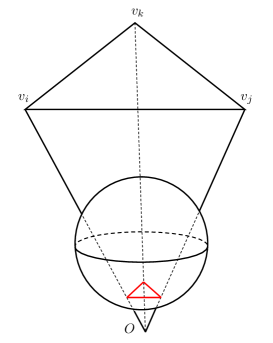
As a byproduct of Theorem 1.1, we prove some new convexity of the volume of generalized hyperbolic pyramids with right-angled hyperbolic hexagonal bases. Suppose $Ov_{i}v_{j}v_{k}$ is a generalized hyperbolic tetrahedron satisfying (1) all the vertices $O$ , $v_{i}$ , $v_{j}$ , $v_{k}$ are hyper-ideal, (2) the intersection of the hyperbolic plane $P_{O}$ dual to $O$ and $\mathbb{H}^{3}$ is a generalized hyperbolic triangle with all vertices hyper-ideal and edges intersecting with $\mathbb{H}^{3}$ . Here and in the following, we use $P_{v}$ to denote the hyperbolic plane dual to a hyper-ideal point $v$ . Please refer to Figure 4 for such a generalized hyperbolic tetrahedron. Truncating the generalized hyperbolic tetrahedron $Ov_{i}v_{j}v_{k}$ with the planes dual to $O$ , $v_{i}$ , $v_{j}$ , $v_{k}$ gives rise to a generalized hyperbolic pyramid $C$ , which has a base given by a right-angled hyperbolic hexagon and an apex $O^{\prime}$ . Please refer to Figure 2 for the resulting generalized hyperbolic pyramid.

If $O^{\prime}$ is hyper-ideal, we further truncate $C$ by the hyperbolic plane $P_{O^{\prime}}$ dual to $O^{\prime}$ . Otherwise, we keep the generalized hyperbolic pyramid $C$ invariant. Denote the volume of the resulting generalized hyperbolic polyhedra by $V$ and call it the volume of the generalized hyperbolic pyramid $C$ . Further denote the intersection angles of $P_{O}$ with $P_{v_{i}}$ , $P_{v_{j}}$ , $P_{v_{k}}$ by $\alpha_{i}$ , $\alpha_{j}$ and $\alpha_{k}$ respectively, which are dihedral angles of the generalized hyperbolic pyramid $C$ at the edges $P_{O}\cap P_{v_{i}}$ , $P_{O}\cap P_{v_{j}}$ , $P_{O}\cap P_{v_{k}}$ respectively.

Theorem 1.2.

The volume $V$ of the generalized hyperbolic pyramid $C$ is a strictly concave function of the dihedral angles $\alpha_{i}$ , $\alpha_{j}$ and $\alpha_{k}$ .

Since Chow-Luo’s pioneering work [2] on combinatorial Ricci flows for Thurston’s circle packings and Luo’s work [16] on combinatorial Yamabe flow for vertex scaling of piecewise linear metrics on closed surfaces, combinatorial curvature flows have been important approaches for constructing geometrical structures on surfaces. There are lots of important works on combinatorial curvature flows on surfaces. See, for instance, [2, 16, 10, 9, 35, 3, 4, 5, 6, 40, 31, 13, 15, 20] and others. Aiming at finding hyperbolic metrics on surfaces with totally geodesic boundary components of prescribed lengths, we introduce the following combinatorial curvature flows to deform the discrete conformal structures in Definition 1, including combinatorial Ricci flow, combinatorial Calabi flow and fractional combinatorial Calabi flow. Set

\alpha_{i}=\arctan e^{-u_{i}},\alpha_{i}\in(0,\frac{\pi}{2}).

(1.3)

By Definition 1 and the formula (1.3), we have

\cosh l_{ij}=\frac{\cos\alpha_{i}\cos\alpha_{j}+\eta_{ij}}{\sin\alpha_{i}\sin\alpha_{j}}.

(1.4)

The formula (1.4) motivates a nice geometric interpolation in $3$ -dimensional hyperbolic geometry in Section 6 for the discrete conformal structures in Definition 1. For simplicity, we also call the function $\alpha:B\rightarrow(0,\frac{\pi}{2})$ in (1.3) as a discrete conformal factor, if it causes no confusion in the context.

Definition 2.

Suppose $(\Sigma,\mathcal{T})$ is an ideally triangulated surface with boundary and $\eta:E\rightarrow(-1,+\infty)$ is a weight defined on the edges. The combinatorial Ricci flow for the discrete conformal structures in Definition 1 on $(\Sigma,\mathcal{T},\eta)$ is defined to be

\displaystyle\left\{\begin{array}[]{ll}\frac{d\alpha_{i}}{dt}=\overline{K}_{i}-K_{i},&\hbox{ }\\ \alpha(0)=\alpha_{0},&\hbox{ }\end{array}\right.

(1.5)

where $\overline{K}\in\mathbb{R}^{n}_{>0}$ is a positive function defined on $B=\{1,2,\cdots,n\}$ , $\alpha_{0}$ is an admissible discrete conformal factor on $(\Sigma,\mathcal{T},\eta)$ . The combinatorial Calabi flow for the discrete conformal structures in Definition 1 on $(\Sigma,\mathcal{T},\eta)$ is defined to be

\displaystyle\left\{\begin{array}[]{ll}\frac{d\alpha_{i}}{dt}=\Delta(K-\overline{K})_{i},&\hbox{ }\\ \alpha(0)=\alpha_{0},&\hbox{ }\end{array}\right.

(1.6)

where $\Delta=-(\frac{\partial K}{\partial\alpha})$ is the discrete Laplace operator.

In Proposition 4.2, we prove that the discrete Laplace operator $\Delta$ is strictly negative definite under the structure condition (1.2). Following [31], we define the fractional combinatorial Laplace operator $\Delta^{s}$ for $s\in\mathbb{R}$ as follows. Recall that a symmetric positive definite matrix $A_{n\times n}$ could be written as

A=P^{T}\cdot\text{diag}\{\lambda_{1},\cdots,\lambda_{n}\}\cdot P,

where $P\in O(n)$ and $\lambda_{1}\leq\cdots\leq\lambda_{n}$ are positive eigenvalues of $A$ . For any $s\in\mathbb{R}$ , $A^{s}$ is defined to be

A^{s}=P^{T}\cdot\text{diag}\{\lambda_{1}^{s},\cdots,\lambda_{n}^{s}\}\cdot P.

The $2s$ -th order fractional discrete Laplace operator $\Delta^{s}$ is defined to be

\Delta^{s}=-\left(\frac{\partial K}{\partial\alpha}\right)^{s}.

(1.7)

Motivated by [31], we introduce the following fractional combinatorial Calabi flow for the discrete conformal structures in Definition 1 on $(\Sigma,\mathcal{T},\eta)$

\displaystyle\left\{\begin{array}[]{ll}\frac{d\alpha_{i}}{dt}=\Delta^{s}(K-\overline{K})_{i},&\hbox{ }\\ \alpha(0)=\alpha_{0},&\hbox{ }\end{array}\right.

(1.8)

where $\Delta^{s}$ is the fractional discrete Laplace operator defined by (1.7). If $s=0$ , the fractional combinatorial Calabi flow (1.8) is reduced to the combinatorial Ricci flow (1.5). If $s=1$ , the fractional combinatorial Calabi flow (1.8) is reduced to the combinatorial Calabi flow (1.6). We have the following result on the combinatorial curvatures flows.

Theorem 1.3.

Suppose $(\Sigma,\mathcal{T})$ is an ideally triangulated surface with boundary and $\eta:E\rightarrow(-1,+\infty)$ is a weight defined on the edges satisfying the structure condition (1.2).

(a): The combinatorial Ricci flow (1.5) and the combinatorial Calabi flow (1.6) are negative gradient flows.
(b): Suppose there exists an admissible discrete conformal structure $\overline{\alpha}$ such that $K(\overline{\alpha})=\overline{K}$ , then there exists a positive number $\delta$ such that if $||\alpha_{0}-\overline{\alpha}||<\delta$ , the solutions of the combinatorial Ricci flow (1.5), the combinatorial Calabi flow (1.6) and the fractional combinatorial Calabi flow (1.8) exist for all time and converge exponentially fast to $\overline{\alpha}$ .
(c): The solutions of the combinatorial Ricci flow (1.5), the combinatorial Calabi flow (1.6) and the fractional combinatorial Calabi flow (1.8) can not reach the boundary of the admissible space of discrete conformal factors $\alpha$ in $(0,\frac{\pi}{2})^{n}$ .

The paper is organized as follows. In Section 2, we give a characterization of the admissible space of discrete conformal factors on ideally triangulated surfaces. In Section 3, we prove that the Jacobian matrix of the generalized inner angles with respect to the discrete conformal factors in a generalized hyperbolic triangle (right-angled hyperbolic hexagon) is symmetric and positive definite. In Section 4, we prove the global rigidity of the generalized combinatorial curvature, i.e. Theorem 1.1. In Section 5, we study the properties of the solutions to the combinatorial Ricci flow (1.5), combinatorial Calabi flow (1.6) and fractional combinatorial Calabi flow (1.8) on ideally triangulated surfaces with boundary and prove Theorem 1.3. In Section 6, we study the relationships between the discrete conformal structures in Definition 1 and $3$ -dimensional hyperbolic space. As a result, we prove some new convexity of the volume of some generalized hyperbolic pyramids with right-angled hyperbolic hexagonal base in dihedral angles, i.e. Theorem 1.2. In Section 7, we discuss some interesting open problems on hyperbolic discrete conformal structures on surfaces with boundary.

Acknowledgements
The research of the author is supported by the Fundamental Research Funds for the Central Universities under Grant no. 2042020kf0199.

2 The admissible space of discrete conformal factors

We denote the space of functions $\alpha:B\rightarrow(0,\frac{\pi}{2})$ such that

\displaystyle\frac{\cos\alpha_{i}\cos\alpha_{j}+\eta_{ij}}{\sin\alpha_{i}\sin\alpha_{j}}>1

(2.1)

for the edge $\{ij\}\in E$ as $\mathcal{W}^{\alpha}_{ij}$ and denote the space of admissible discrete conformal factor $\alpha:B\rightarrow(0,\frac{\pi}{2})$ as $\mathcal{W}^{\alpha}$ .

Theorem 2.1.

Suppose $(\Sigma,\mathcal{T})$ is an ideally triangulated surface with boundary and $\eta:E\rightarrow(-1,+\infty)$ is a weight defined on the edges. For each edge $\{ij\}\in E$ , the space $\mathcal{W}^{\alpha}_{ij}$ is a convex polytope in $(0,\frac{\pi}{2})^{n}$ . As a result, the admissible space

\mathcal{W}^{\alpha}=\cap_{\{ij\}\in E}\mathcal{W}^{\alpha}_{ij}

is a convex polytope in $(0,\frac{\pi}{2})^{n}$ .

Proof. By the definition of $\alpha$ in (1.3), a function $\alpha:B\rightarrow(0,\frac{\pi}{2})$ belongs to $\mathcal{W}^{\alpha}_{ij}$ if and only if (2.1) is valid, which is equivalent to

\cos(\alpha_{i}+\alpha_{j})>-\eta_{ij}.

(2.2)

If $-\eta_{ij}<-1$ , i.e. $\eta_{ij}>1$ , the condition (2.2) is satisfied for any $\alpha_{i},\alpha_{j}\in(0,\frac{\pi}{2})$ . If $-\eta_{ij}\geq-1$ , i.e. $-1<\eta_{ij}\leq 1$ , then the condition (2.2) implies that $\alpha_{i}+\alpha_{j}<\arccos(-\eta_{ij}).$ In any case, for the edge $\{ij\}\in E$ , the space

\mathcal{W}^{\alpha}_{ij}=\{\alpha\in(0,\frac{\pi}{2})^{n}|\cos(\alpha_{i}+\alpha_{j})>-\eta_{ij}\}

(2.3)

is a convex polytope in $(0,\frac{\pi}{2})^{2}$ . $\square$

Remark 2.

The admissible space $\mathcal{W}^{\alpha}$ is nonempty. Especially, $\mathcal{W}^{\alpha}$ contains the points $\alpha\in(0,\frac{\pi}{2})^{n}$ with all $\alpha_{i}$ small enough. One can also use (1.4) as the definition of discrete conformal structures on ideally triangulated surfaces with boundary with $\alpha\in(0,\pi)$ as a discrete conformal factor instead of (1.1), which corresponds to $\alpha\in(0,\frac{\pi}{2})$ . Following the proof of Theorem 2.1, we can also prove that the admissible space of discrete conformal factors $\alpha$ is a convex polytope in $(0,\pi)^{n}$ in this case. This definition of discrete conformal structures is reasonable from the viewpoint of 3-dimensional hyperbolic geometry in Section 6. However, we can not prove the rigidity for the generalized combinatorial curvature in this setting. Please refer to Remark 5.

3 Jacobian matrix of the generalized angles in a generalized hyperbolic triangle

Suppose $\{ijk\}\in F$ is a generalized hyperbolic triangle with hyper-ideal vertices $i,j,k$ , which corresponds to a right-angled hyperbolic hexagon adjacent the boundary components $i,j,k\in B$ . The length of the boundary arc in $\{ijk\}\in F$ facing the edge $\{jk\}$ is called the generalized angle of the generalized hyperbolic triangle $\{ijk\}$ at $i$ . Denote the edge lengths of three nonadjacent edges $\{ij\},\{ik\},\{jk\}$ as $l_{ij},l_{ik},l_{jk}$ respectively and the generalized inner angles at the hyper-ideal vertices $i,j,k$ as $\theta_{i}$ , $\theta_{j}$ , $\theta_{k}$ respectively.

3.1 Symmetry of the Jacobian matrix

Set

\gamma_{i}=\eta_{jk}+\eta_{ij}\eta_{ik}.

We have the following result on the symmetry of the Jacobian matrix $\frac{\partial(\theta_{i},\theta_{j},\theta_{k})}{\partial(\alpha_{i},\alpha_{j},\alpha_{k})}$

Lemma 3.1.

For discrete conformal factor $\alpha\in\mathcal{W}^{\alpha}_{ij}\cap\mathcal{W}^{\alpha}_{ik}\cap\mathcal{W}^{\alpha}_{jk}$ ,

\displaystyle\frac{\partial\theta_{i}}{\partial\alpha_{j}}=\frac{\partial\theta_{j}}{\partial\alpha_{i}}=\frac{1}{A_{ijk}\sinh^{2}l_{ij}\sin^{2}\alpha_{i}\sin^{2}\alpha_{j}\sin\alpha_{k}}[(1-\eta^{2}_{ij})\cos\alpha_{k}+\gamma_{i}\cos\alpha_{j}+\gamma_{j}\cos\alpha_{i}],

where $A_{ijk}=\sinh l_{ij}\sinh l_{ik}\sinh\theta_{i}$ .

Proof. By the derivative cosine law for right-angled hyperbolic hexagons [14], we have

\displaystyle\frac{\partial\theta_{i}}{\partial l_{ij}}=\frac{-\sinh l_{jk}\cosh\theta_{j}}{A_{ijk}},\ \frac{\partial\theta_{i}}{\partial l_{ik}}=\frac{-\sinh l_{jk}\cosh\theta_{k}}{A_{ijk}},\ \frac{\partial\theta_{i}}{\partial l_{jk}}=\frac{\sinh l_{jk}}{A_{ijk}}.

(3.1)

By the formula (1.4) of the hyperbolic length in discrete conformal factor $\alpha$ , we have

\displaystyle\frac{\partial l_{ij}}{\partial\alpha_{j}}=-\frac{\cos\alpha_{i}+\eta_{ij}\cos\alpha_{j}}{\sinh l_{ij}\sin\alpha_{i}\sin^{2}\alpha_{j}},\ \frac{\partial l_{ik}}{\partial\alpha_{j}}=0,\ \frac{\partial l_{jk}}{\partial\alpha_{j}}=-\frac{\cos\alpha_{k}+\eta_{jk}\cos\alpha_{j}}{\sinh l_{jk}\sin^{2}\alpha_{j}\sin\alpha_{k}}.

(3.2)

By the chain rules, we have

\displaystyle\frac{\partial\theta_{i}}{\partial\alpha_{j}}=\frac{\partial\theta_{i}}{\partial l_{ij}}\frac{\partial l_{ij}}{\partial\alpha_{j}}+\frac{\partial\theta_{i}}{\partial l_{ik}}\frac{\partial l_{ik}}{\partial\alpha_{j}}+\frac{\partial\theta_{i}}{\partial l_{jk}}\frac{\partial l_{jk}}{\partial\alpha_{j}}=\frac{\partial\theta_{i}}{\partial l_{ij}}\frac{\partial l_{ij}}{\partial\alpha_{j}}+\frac{\partial\theta_{i}}{\partial l_{jk}}\frac{\partial l_{jk}}{\partial\alpha_{j}}.

(3.3)

Submitting (3.1) and (3.2) into (3.3) gives

	$\displaystyle\frac{\partial\theta_{i}}{\partial\alpha_{j}}=$	$\displaystyle\frac{\sinh l_{jk}\cosh\theta_{j}}{A_{ijk}}\cdot\frac{\cos\alpha_{i}+\eta_{ij}\cos\alpha_{j}}{\sinh l_{ij}\sin\alpha_{i}\sin^{2}\alpha_{j}}-\frac{\sinh l_{jk}}{A_{ijk}}\cdot\frac{\cos\alpha_{k}+\eta_{jk}\cos\alpha_{j}}{\sinh l_{jk}\sin^{2}\alpha_{j}\sin\alpha_{k}}$		(3.4)
	$\displaystyle=$	$\displaystyle\frac{\cos\alpha_{i}+\eta_{ij}\cos\alpha_{j}}{A_{ijk}\sinh^{2}l_{ij}\sin\alpha_{i}\sin^{2}\alpha_{j}}[\cosh l_{ij}\cosh l_{jk}+\cosh l_{ik}]-\frac{\cos\alpha_{k}+\eta_{jk}\cos\alpha_{j}}{A_{ijk}\sin^{2}\alpha_{j}\sin\alpha_{k}},$		(3.4)

where the cosine law for right-angled hyperbolic hexagons is used in the last line. Submitting (1.4) into (3.4), by lengthy but direct calculations, we have

	$\displaystyle\frac{\partial\theta_{i}}{\partial\alpha_{j}}=$	$\displaystyle\frac{1}{A_{ijk}\sinh^{2}l_{ij}\sin^{2}\alpha_{i}\sin^{2}\alpha_{j}\sin\alpha_{k}}$		(3.5)
		$\displaystyle\cdot[(1-\eta^{2}_{ij})\cos\alpha_{k}+(\eta_{ik}+\eta_{ij}\eta_{jk})\cos\alpha_{i}+(\eta_{jk}+\eta_{ij}\eta_{ik})\cos\alpha_{j}].$		(3.5)

Note that $A_{ijk}$ is symmetric in $i,j,k$ by the sine law for right-angled hyperbolic hexagons, we have $\frac{\partial\theta_{i}}{\partial\alpha_{j}}=\frac{\partial\theta_{j}}{\partial\alpha_{i}}$ by (3.5). $\square$

Remark 3.

Lemma 3.1 is still valid if we use (1.4) as the definition of discrete conformal structures on ideally triangulated surfaces with boundary with $\alpha\in(0,\pi)$ .

As a direct corollary of Lemma 3.1, we have the following result.

Corollary 3.2.

If the weight $\eta\in(-1,1]$ and satisfies the structure condition (1.2), then

\frac{\partial\theta_{i}}{\partial\alpha_{j}}\geq 0,

the equality of which is attained if and only if $\eta_{ij}=1$ and $\eta_{ik}+\eta_{jk}=0$ .

In the special case of $\eta\equiv 0$ , we further have the following interesting formula on the relationships between $\frac{\partial\theta_{i}}{\partial\alpha_{i}}$ , $\frac{\partial\theta_{i}}{\partial\alpha_{j}}$ and $\frac{\partial\theta_{i}}{\partial\alpha_{k}}$ .

Lemma 3.3.

If $\eta\equiv 0$ , for discrete conformal factor $\alpha\in\mathcal{W}^{\alpha}_{ij}\cap\mathcal{W}^{\alpha}_{ik}\cap\mathcal{W}^{\alpha}_{jk}$ , we have

\displaystyle\frac{\partial\theta_{i}}{\partial\alpha_{i}}=\frac{\partial\theta_{i}}{\partial\alpha_{j}}\cosh l_{ij}+\frac{\partial\theta_{i}}{\partial\alpha_{k}}\cosh l_{ik}.

(3.6)

Proof. By Lemma 3.1, we have

\displaystyle\frac{\partial\theta_{i}}{\partial\alpha_{j}}=\frac{\cot\alpha_{k}}{A_{ijk}\sinh^{2}l_{ij}\sin^{2}\alpha_{i}\sin^{2}\alpha_{j}},\frac{\partial\theta_{i}}{\partial\alpha_{k}}=\frac{\cot\alpha_{j}}{A_{ijk}\sinh^{2}l_{ik}\sin^{2}\alpha_{i}\sin^{2}\alpha_{k}}

(3.7)

in the case of $\eta\equiv 0$ . By the chain rules, we have

$\displaystyle\frac{\partial\theta_{i}}{\partial\alpha_{i}}=$	$\displaystyle\frac{\partial\theta_{i}}{\partial l_{ij}}\frac{\partial l_{ij}}{\partial\alpha_{i}}+\frac{\partial\theta_{i}}{\partial l_{ik}}\frac{\partial l_{ik}}{\partial\alpha_{i}}+\frac{\partial\theta_{i}}{\partial l_{jk}}\frac{\partial l_{jk}}{\partial\alpha_{i}}$	(3.8)
$\displaystyle=$	$\displaystyle\frac{\sinh l_{jk}\cosh\theta_{j}}{A_{ijk}}\frac{\cos\alpha_{j}+\eta_{ij}\cos\alpha_{i}}{\sinh l_{ij}\sin^{2}\alpha_{i}\sin\alpha_{j}}+\frac{\sinh l_{jk}\cosh\theta_{k}}{A_{ijk}}\frac{\cos\alpha_{k}+\eta_{ik}\cos\alpha_{i}}{\sinh l_{ik}\sin^{2}\alpha_{i}\sin\alpha_{k}}$
$\displaystyle=$	$\displaystyle\frac{1}{A_{ijk}\sinh^{2}l_{ij}\sin^{2}\alpha_{i}\sin\alpha_{j}}(\cosh l_{ij}\cosh l_{jk}+\cosh l_{ik})(\cos\alpha_{j}+\eta_{ij}\cos\alpha_{i})$
	$\displaystyle+\frac{1}{A_{ijk}\sinh^{2}l_{ik}\sin^{2}\alpha_{i}\sin\alpha_{k}}(\cosh l_{ik}\cosh l_{jk}+\cosh l_{ij})(\cos\alpha_{k}+\eta_{ik}\cos\alpha_{i})$

Submitting (1.4) and $\eta\equiv 0$ into (3.8), by lengthy but direct calculations, we have

\displaystyle\frac{\partial\theta_{i}}{\partial\alpha_{i}}=\frac{\cot\alpha_{i}\cot\alpha_{j}\cot\alpha_{k}}{A_{ijk}\sinh^{2}l_{ij}\sin^{2}\alpha_{i}\sin^{2}\alpha_{j}}+\frac{\cot\alpha_{i}\cot\alpha_{j}\cot\alpha_{k}}{A_{ijk}\sinh^{2}l_{ik}\sin^{2}\alpha_{i}\sin^{2}\alpha_{k}}.

(3.9)

Note that

\displaystyle\cosh l_{ij}=\cot\alpha_{i}\cot\alpha_{j},\cosh l_{ik}=\cot\alpha_{i}\cot\alpha_{k}

(3.10)

in the case of $\eta\equiv 0$ by (1.4). Combining the formulae (3.7), (3.9) and (3.10) gives the formula (3.6). $\square$

Remark 4.

The formula (3.6) was first obtained by Glickenstein-Thomas [8] (see also [27]) for generic hyperbolic discrete conformal structures on closed surfaces, which has lots of applications. See, for instance, [31, 35, 34, 36, 37] and others. This is the first time the formula (3.6) proved for hyperbolic discrete conformal structures on surfaces with boundary. It is conceived that the formula (3.6) holds for any hyperbolic discrete conformal structures on ideally triangulated surfaces with boundary.

3.2 Positive definiteness of the Jacobian matrix

The aim of this subsection is to prove that the Jacobian matrix $\frac{\partial(\theta_{i},\theta_{j},\theta_{k})}{\partial(u_{i},u_{j},u_{k})}$ for a generalized triangle $\{ijk\}\in F$ is positive definite for admissible discrete conformal factors.

Lemma 3.4.

Suppose $\{ijk\}\in F$ is a generalized triangle adjacent to $i,j,k\in B$ and $\eta\in(-1,+\infty)$ is a weight defined on the edges satisfying the structure condition (1.2), then the Jacobian matrix $\frac{\partial(\theta_{i},\theta_{j},\theta_{k})}{\partial(\alpha_{i},\alpha_{j},\alpha_{k})}$ is nonsingular with positive determinant for any discrete conformal factor $\alpha\in\mathcal{W}^{\alpha}_{ij}\cap\mathcal{W}^{\alpha}_{ik}\cap\mathcal{W}^{\alpha}_{jk}$ .

Proof. By the chain rules, we have

\displaystyle\frac{\partial(\theta_{i},\theta_{j},\theta_{k})}{\partial(\alpha_{i},\alpha_{j},\alpha_{k})}=\frac{\partial(\theta_{i},\theta_{j},\theta_{k})}{\partial(l_{ij},l_{ik},l_{jk})}\cdot\frac{\partial(l_{ij},l_{ik},l_{jk})}{\partial(\alpha_{i},\alpha_{j},\alpha_{k})}.

(3.11)

By the proof of Lemma 3.1, we have

	$\displaystyle\left(\begin{array}[]{c}d\theta_{i}\\ d\theta_{j}\\ d\theta_{k}\\ \end{array}\right)=$	$\displaystyle\frac{-1}{\sinh l_{ij}\sinh l_{ik}\sinh\theta_{i}}$		(3.12)
		$\displaystyle\cdot\left(\begin{array}[]{ccc}\sinh l_{jk}&0&0\\ 0&\sinh l_{ik}&0\\ 0&0&\sinh l_{ij}\\ \end{array}\right)\left(\begin{array}[]{ccc}\cosh\theta_{j}&\cosh\theta_{k}&-1\\ \cosh\theta_{i}&-1&\cosh\theta_{k}\\ -1&\cosh\theta_{i}&\cosh\theta_{j}\\ \end{array}\right)\left(\begin{array}[]{c}dl_{ij}\\ dl_{ik}\\ dl_{jk}\\ \end{array}\right),$		(3.12)

which implies

\displaystyle\det\left(\frac{\partial(\theta_{i},\theta_{j},\theta_{k})}{\partial(l_{ij},l_{ik},l_{jk})}\right)=\left(\frac{-1}{\sinh l_{ij}\sinh l_{ik}\sinh\theta_{i}}\right)^{3}\sinh l_{ij}\sinh l_{ik}\sinh l_{jk}\det M

with $M$ being the last $3\times 3$ matrix in (3.12). By direct calculations, we have

\displaystyle\det M=-\cosh^{2}\theta_{i}-\cosh^{2}\theta_{j}-\cosh^{2}\theta_{k}-2\cosh\theta_{i}\cosh\theta_{j}\cosh\theta_{k}+1<0,

which implies that

\displaystyle\det\left(\frac{\partial(\theta_{i},\theta_{j},\theta_{k})}{\partial(l_{ij},l_{ik},l_{jk})}\right)>0.

(3.13)

On the other hand, by the formula (1.4) of hyperbolic length in $\alpha$ , we have

\displaystyle\left(\begin{array}[]{c}dl_{ij}\\ dl_{ik}\\ dl_{jk}\\ \end{array}\right)=-\left(\begin{array}[]{ccc}\frac{1}{\sinh l_{ij}}&0&0\\ 0&\frac{1}{\sinh l_{ik}}&0\\ 0&0&\frac{1}{\sinh l_{jk}}\\ \end{array}\right)\cdot J\cdot\left(\begin{array}[]{c}d\alpha_{i}\\ d\alpha_{j}\\ d\alpha_{k}\\ \end{array}\right),

where $J$ is the following $3\times 3$ matrix

\displaystyle J=\left(\begin{array}[]{ccc}\cosh l_{ij}\cot\alpha_{i}+\cot\alpha_{j}&\cosh l_{ij}\cot\alpha_{j}+\cot\alpha_{i}&0\\ \cosh l_{ik}\cot\alpha_{i}+\cot\alpha_{k}&0&\cosh l_{ik}\cot\alpha_{k}+\cot\alpha_{i}\\ 0&\cosh l_{jk}\cot\alpha_{j}+\cot\alpha_{k}&\cosh l_{jk}\cot\alpha_{k}+\cot\alpha_{j}\\ \end{array}\right).

By lengthy but direct calculations, we have

	$\displaystyle\det\left(\frac{\partial(l_{ij},l_{ik},l_{jk})}{\partial(\alpha_{i},\alpha_{j},\alpha_{k})}\right)$	(3.14)
$\displaystyle=$	$\displaystyle\frac{-1}{\sinh l_{ij}\sinh l_{ik}\sinh l_{jk}}\det J$
$\displaystyle=$	$\displaystyle\frac{1}{\sinh l_{ij}\sinh l_{ik}\sinh l_{jk}\sin^{3}\alpha_{i}\sin^{3}\alpha_{j}\sin^{3}\alpha_{j}}$
	$\displaystyle\cdot[2(1+\eta_{ij}\eta_{ik}\eta_{jk})\cos\alpha_{i}\cos\alpha_{j}\cos\alpha_{k}+\gamma_{i}\cos\alpha_{i}(\cos^{2}\alpha_{j}+\cos^{2}\alpha_{k})$
	$\displaystyle\ \ \ +\gamma_{j}\cos\alpha_{j}(\cos^{2}\alpha_{i}+\cos^{2}\alpha_{k})+\gamma_{k}\cos\alpha_{k}(\cos^{2}\alpha_{i}+\cos^{2}\alpha_{j})].$

Note that $\alpha_{i},\alpha_{j},\alpha_{k}\in(0,\frac{\pi}{2})$ by (1.3) and $\gamma_{i}\geq 0,\gamma_{j}\geq 0,\gamma_{k}\geq 0$ by the structure condition (1.2), we have

	$\displaystyle\det\left(\frac{\partial(l_{ij},l_{ik},l_{jk})}{\partial(\alpha_{i},\alpha_{j},\alpha_{k})}\right)$	(3.15)
$\displaystyle\geq$	$\displaystyle\frac{2\cos\alpha_{i}\cos\alpha_{j}\cos\alpha_{k}}{\sinh l_{ij}\sinh l_{ik}\sinh l_{jk}\sin^{3}\alpha_{i}\sin^{3}\alpha_{j}\sin^{3}\alpha_{j}}$
	$\displaystyle\cdot(1+\eta_{ij}\eta_{ik}\eta_{jk}+\eta_{jk}+\eta_{ij}\eta_{ik}+\eta_{ij}+\eta_{ik}\eta_{jk}+\eta_{ik}+\eta_{ij}\eta_{jk})$
$\displaystyle=$	$\displaystyle\frac{2\cos\alpha_{i}\cos\alpha_{j}\cos\alpha_{k}}{\sinh l_{ij}\sinh l_{ik}\sinh l_{jk}\sin^{3}\alpha_{i}\sin^{3}\alpha_{j}\sin^{3}\alpha_{j}}(1+\eta_{ij})(1+\eta_{ik})(1+\eta_{jk})$
$\displaystyle>$	$\displaystyle 0$

by (3.14), where the conditions $\eta\in(-1,+\infty)$ and $\alpha_{i},\alpha_{j},\alpha_{k}\in(0,\frac{\pi}{2})$ are used in the last line. Combining the equations (3.13) and (3.15) gives

\det\left(\frac{\partial(\theta_{i},\theta_{j},\theta_{k})}{\partial(\alpha_{i},\alpha_{j},\alpha_{k})}\right)>0

by (3.11), which implies that the Jacobian matrix $\frac{\partial(\theta_{i},\theta_{j},\theta_{k})}{\partial(\alpha_{i},\alpha_{j},\alpha_{k})}$ is nonsingular. $\square$

Remark 5.

By Remark 2, we can define the discrete conformal structure using the formula (1.4) with $\alpha_{i}\in(0,\pi)$ . However, in this case, we do not have $\cos\alpha_{i}>0$ , which is technically necessary in the proof of Lemma 3.4.

To prove that the Jacobian matrix $\frac{\partial(\theta_{i},\theta_{j},\theta_{k})}{\partial(\alpha_{i},\alpha_{j},\alpha_{k})}$ is positive definite, following [35, 34], we further introduce the following parameterized admissible space

\mathcal{A}_{ijk}=\{(\alpha_{i},\alpha_{j},\alpha_{k},\eta_{ij},\eta_{ik},\eta_{jk})\in\mathcal{W}^{\alpha}_{ijk}(\eta)\times(-1,+\infty)^{3}|\gamma_{i}\geq 0,\gamma_{j}\geq 0,\gamma_{k}\geq 0\}

for a generalized triangle $\{ijk\}\in F$ , where we use $\mathcal{W}^{\alpha}_{ijk}(\eta)$ to denote $\mathcal{W}^{\alpha}_{ij}\cap\mathcal{W}^{\alpha}_{ik}\cap\mathcal{W}^{\alpha}_{jk}$ depending on $\eta$ for simplicity. The parameterized admissible space $\mathcal{A}_{ijk}$ can be taken as a fibre bundle over the space

\Gamma:=\{(\eta_{ij},\eta_{ik},\eta_{jk})\in(-1,+\infty)^{3}|\gamma_{i}\geq 0,\gamma_{j}\geq 0,\gamma_{k}\geq 0\}

with the fibre given by $\mathcal{W}^{\alpha}_{ijk}(\eta)$ over $\eta\in\Gamma$ .

Lemma 3.5 ([34] Lemma 2.7).

The space $\Gamma$ is path connected.

As a direct corollary of Lemma 3.5, we have the following result.

Corollary 3.6.

Suppose $\{ijk\}\in F$ is a generalized triangle adjacent to $i,j,k\in B$ . Then the parameterized admissible space $\mathcal{A}_{ijk}$ is connected.

Proof. Set

f_{ij}(\alpha,\eta)=\frac{\cos\alpha_{i}\cos\alpha_{j}+\eta_{ij}}{\sin\alpha_{i}\sin\alpha_{j}}.

Then $(\alpha_{i},\alpha_{j},\alpha_{k},\eta_{ij},\eta_{ik},\eta_{jk})\in\mathcal{A}_{ijk}$ if and only if $f_{ij}>1$ , $f_{ik}>1$ , $f_{jk}>1$ . By the continuity of $f_{ij},f_{ik},f_{jk}$ , if $(\alpha_{i},\alpha_{j},\alpha_{k},\eta_{ij},\eta_{ik},\eta_{jk})\in\mathcal{A}_{ijk}$ , then there is a convex neighborhood $U$ of $(\alpha_{i},\alpha_{j},\alpha_{k},\eta_{ij},\eta_{ik},\eta_{jk})$ such that $U\subseteq\mathcal{A}_{ijk}$ . As a result, for any fixed point $(\overline{\alpha}_{i},\overline{\alpha}_{j},\overline{\alpha}_{k})\in\mathcal{W}^{\alpha}_{ijk}(\eta_{0})$ , there is a connected neighborhood $V$ of $\eta_{0}$ in $\Gamma$ such that the space

\{(\overline{\alpha}_{i},\overline{\alpha}_{j},\overline{\alpha}_{k},\eta_{ij},\eta_{ik},\eta_{jk})\in\mathcal{A}_{ijk}|(\overline{\alpha}_{i},\overline{\alpha}_{j},\overline{\alpha}_{k})\in\mathcal{W}^{\alpha}_{ijk}(\eta),(\eta_{ij},\eta_{ik},\eta_{jk})\in V\}

is connected. Then the connectivity of the parameterized admissible space $\mathcal{A}_{ijk}$ follows from Theorem 2.1 and Lemma 3.5. $\square$

Theorem 3.7.

Suppose $\{ijk\}\in F$ is a generalized hyperbolic triangle adjacent to $i,j,k\in B$ and $\eta\in(-1,+\infty)$ is a weight defined on the edges satisfying the structure condition (1.2). Then the Jacobian matrix

\frac{\partial(\theta_{i},\theta_{j},\theta_{k})}{\partial(\alpha_{i},\alpha_{j},\alpha_{k})}

is strictly positive definite for any discrete conformal factor in $\mathcal{W}^{\alpha}_{ij}\cap\mathcal{W}^{\alpha}_{ik}\cap\mathcal{W}^{\alpha}_{jk}$ .

Proof. Note that the Jacobian matrix $\frac{\partial(\theta_{i},\theta_{j},\theta_{k})}{\partial(\alpha_{i},\alpha_{j},\alpha_{k})}$ can be taken as a matrix-valued function defined on the parameterized admissible space $\mathcal{A}_{ijk}$ . By Lemma 3.4 and Corollary 3.6, the eigenvalues of $\frac{\partial(\theta_{i},\theta_{j},\theta_{k})}{\partial(\alpha_{i},\alpha_{j},\alpha_{k})}$ are nonzero continuous functions defined on the connected parameterized admissible space $\mathcal{A}_{ijk}$ . To prove that $\frac{\partial(\theta_{i},\theta_{j},\theta_{k})}{\partial(\alpha_{i},\alpha_{j},\alpha_{k})}$ is positive definite, we just need to choose a point $p$ in $\mathcal{A}_{ijk}$ such that $\frac{\partial(\theta_{i},\theta_{j},\theta_{k})}{\partial(\alpha_{i},\alpha_{j},\alpha_{k})}$ is positive definite at $p$ .

Take $p=(\alpha_{i},\alpha_{j},\alpha_{k},0,0,0)\in\mathcal{A}_{ijk}$ . By Lemma 3.1, we have

\frac{\partial\theta_{i}}{\partial\alpha_{j}}>0,\frac{\partial\theta_{i}}{\partial\alpha_{k}}>0

(3.16)

at $p$ . By Lemma 3.3, we further have

\frac{\partial\theta_{i}}{\partial\alpha_{i}}>\frac{\partial\theta_{i}}{\partial\alpha_{j}}+\frac{\partial\theta_{i}}{\partial\alpha_{k}}>0

at $p$ by (3.16), which implies that the Jacobian matrix $\frac{\partial(\theta_{i},\theta_{j},\theta_{k})}{\partial(\alpha_{i},\alpha_{j},\alpha_{k})}$ is diagonal dominant and then positive definite at $p$ . $\square$

4 Rigidity of discrete conformal structures

In this section, we give a proof of Theorem 1.1.

Proof of Theorem 1.1: By Lemma 3.1, $\theta_{i}d\alpha_{i}+\theta_{j}d\alpha_{j}+\theta_{k}d\alpha_{k}$ is a smooth closed $1$ -form on $\mathcal{W}^{\alpha}_{ij}\cap\mathcal{W}^{\alpha}_{ik}\cap\mathcal{W}^{\alpha}_{jk}$ . By Theorem 2.1, the function

\mathcal{E}_{ijk}(\alpha_{i},\alpha_{j},\alpha_{k})=\int^{(\alpha_{i},\alpha_{j},\alpha_{k})}\theta_{i}d\alpha_{i}+\theta_{j}d\alpha_{j}+\theta_{k}d\alpha_{k}

is a well-defined smooth function on $\mathcal{W}^{\alpha}_{ij}\cap\mathcal{W}^{\alpha}_{ik}\cap\mathcal{W}^{\alpha}_{jk}$ with $\nabla\mathcal{E}_{ijk}=(\theta_{i},\theta_{j},\theta_{k})$ , which is strictly convex by Theorem 3.7. Set

\mathcal{E}(\alpha)=\sum_{\{ijk\}\in F}\mathcal{E}_{ijk}(\alpha_{i},\alpha_{j},\alpha_{k})

(4.1)

for $\alpha\in\mathcal{W}^{\alpha}$ . Then $\mathcal{E}(\alpha)$ is a strictly convex smooth function defined on the convex admissible space $\mathcal{W}^{\alpha}$ with the gradient given by

\nabla\mathcal{E}=K.

Then the global rigidity of the generalized combinatorial curvature $K$ follows from the following well-known result in analysis.

Lemma 4.1.

If $W:\Omega\rightarrow\mathbb{R}$ is a $C^{2}$ -smooth strictly convex function defined on a convex domain $\Omega\subseteq\mathbb{R}^{n}$ , then its gradient $\nabla W:\Omega\rightarrow\mathbb{R}^{n}$ is injective.

$\square$

In the proof of Theorem 1.1, we have proved the following result on the Jacobian matrix $(\frac{\partial K}{\partial\alpha})$ .

Proposition 4.2.

Suppose $(\Sigma,\mathcal{T})$ is an ideally triangulated surface with boundary and $\eta:E\rightarrow(-1,+\infty)$ is a weight defined on the edges satisfying the structure condition (1.2). Then the Jacobian matrix $(\frac{\partial K}{\partial\alpha})$ is symmetric and strictly positive definite on the admissible space $\mathcal{W}^{\alpha}$ .

5 Combinatorial curvature flows on surfaces with boundary

In this section, we study some basic properties of the combinatorial Ricci flow (1.5), the combinatorial Calabi flow (1.6), the fractional combinatorial Calabi flow (1.8) and give a proof of Theorem 1.3.

Lemma 5.1.

The combinatorial Ricci flow (1.5) is a negative gradient flow of the convex energy function defined by

\overline{\mathcal{E}}(\alpha)=\mathcal{E}(\alpha)-\sum_{i\in B}\overline{K}_{i}\alpha_{i},

where $\mathcal{E}(\alpha)$ is defined by the formula (4.1).

Proof. By the proof of Theorem 1.1, $\overline{\mathcal{E}}(\alpha)$ is a smooth convex function with

\nabla\overline{\mathcal{E}}=K-\overline{K},

which implies that the combinatorial Ricci flow (1.5) is a negative gradient flow of the convex energy function $\overline{\mathcal{E}}(\alpha)$ . $\square$

Corollary 5.2.

The energy function $\overline{\mathcal{E}}(\alpha)$ is decreasing along the combinatorial Ricci flow (1.5). Furthermore, the generalized combinatorial Calabi energy $\mathcal{C}(\alpha)$ defined by

\mathcal{C}(\alpha)=\frac{1}{2}\sum_{i\in B}(K_{i}-\overline{K}_{i})^{2}

is decreasing along the combinatorial Ricci flow (1.5).

Proof. The monotonicity of $\overline{\mathcal{E}}(\alpha)$ along the combinatorial Ricci flow (1.5) follows from Lemma 5.1. For the generalized combinatorial Calabi energy $\mathcal{C}(\alpha)$ , by direct calculations, we have

\frac{d\mathcal{C}(\alpha(t))}{dt}=\sum_{i\in B}(K_{i}-\overline{K}_{i})\frac{dK_{i}}{dt}=-(K-\overline{K})^{T}\cdot\left(\frac{\partial K}{\partial\alpha}\right)\cdot(K-\overline{K})\leq 0,

along the combinatorial Ricci flow (1.5) by Proposition 4.2, which is strictly negative unless $K=\overline{K}$ . $\square$

Lemma 5.3.

The combinatorial Calabi flow (1.5) is a negative gradient flow of the generalized combinatorial Calabi energy energy $\mathcal{C}(\alpha)$ . As a result, the generalized combinatorial Calabi energy $\mathcal{C}(\alpha)$ is decreasing along the combinatorial Calabi flow (1.6). Furthermore, the energy function $\overline{\mathcal{E}}(\alpha)$ is decreasing along the combinatorial Ricci flow (1.5).

Proof. By direct calculations, we have

\nabla_{\alpha_{i}}\mathcal{C}=\sum_{j\in B}\frac{\partial K_{j}}{\partial\alpha_{i}}(K_{j}-\overline{K}_{j})=-\Delta(K-\overline{K})_{i}

by Proposition 4.2, which implies that the combinatorial Calabi flow (1.5) is a negative gradient flow of $\mathcal{C}(w)$ . Similarly, we have

\frac{d\overline{\mathcal{E}}(\alpha(t))}{dt}=\sum_{i\in B}\nabla_{\alpha_{i}}\overline{\mathcal{E}}\cdot\frac{d\alpha_{i}}{dt}=-(K-\overline{K})^{T}\cdot\left(\frac{\partial K}{\partial\alpha}\right)\cdot(K-\overline{K})\leq 0

by Proposition 4.2, which is strictly negative unless $K=\overline{K}$ . $\square$

Lemma 5.1 and Lemma 5.3 proves Theorem 1.3 (a). Following the arguments in the proof of Lemma 5.1, Corollary 5.2 and Lemma 5.3, we have the following result on the fractional combinatorial Calabi flow (1.8).

Lemma 5.4.

Suppose $(\Sigma,\mathcal{T})$ is an ideally triangulated surface with boundary and $\eta:E\rightarrow(-1,+\infty)$ is a weight defined on the edges satisfying the structure condition (1.2). Then for any $s\in\mathbb{R}$ , the energy function $\overline{\mathcal{E}}(\alpha)$ and the generalized combinatorial Calabi energy $\mathcal{C}(\alpha)$ is decreasing along the fractional combinatorial Calabi flow (1.8).

Remark 6.

For generic $s\in\mathbb{R}$ , except $s=0,1$ , the fractional combinatorial Calabi flow (1.8) is not a gradient flow. Furthermore, as the fractional discrete Laplace operator $\Delta^{s}$ is generically a non-local operator, the definition of which involves the eigenvalues of matrices, the fractional combinatorial Calabi flow (1.8) is generically (except $s=0,1$ ) a non-local combinatorial curvature flow.

Now we give a proof of Theorem 1.3 (b). As the proofs for the combinatorial Ricci flow (1.5), the combinatorial Calabi flow (1.6) and the fractional combinatorial Calabi flow (1.8) are similar, we only give the proof for the fractional combinatorial Calabi flow (1.8) for simplicity.

Proof of Theorem 1.3 (b): Set $\Gamma(\alpha)=\Delta^{s}(K-\overline{K})$ for the fractional combinatorial Calabi flow (1.8). Then $\overline{\alpha}$ is an equilibrium point of the system (1.8) by assumption and

D\Gamma|_{\alpha=\overline{\alpha}}=-\left(\frac{\partial K}{\partial\alpha}\right)(\overline{\alpha}),

which is strictly negative definite by Proposition 4.2. This implies that $\overline{\alpha}$ is a local attractor of the fractional combinatorial Calabi flow (1.8). Then the long time existence of the solution $\alpha(t)$ to (1.8) and the exponential convergence of the solution $\alpha(t)$ to $\overline{\alpha}$ follows from the Lyapunov stability theorem ([21], Chapter 5). $\square$

Recall the characterization (2.3) of the space $\mathcal{W}^{\alpha}_{ij}$ of discrete conformal factors $\alpha:B\rightarrow(0,\frac{\pi}{2})$ such that (2.1) is satisfied for an edge $\{ij\}\in E$ . In the case of $\eta\in(-1,1]$ , $\mathcal{W}^{\alpha}_{ij}$ has a non-empty boundary $\partial\mathcal{W}^{\alpha}_{ij}$ in $(0,\frac{\pi}{2})^{n}$ defined by

\partial\mathcal{W}^{\alpha}_{ij}=\{\alpha\in(0,\frac{\pi}{2})^{n}|\alpha_{i}+\alpha_{j}=\arccos(-\eta_{ij})\}.

Lemma 5.5.

Assume $(\Sigma,\mathcal{T})$ is an ideally triangulated surface with boundary and $\eta:E\rightarrow(-1,+\infty)$ is a weight on the edges with $\eta_{ij}\in(-1,1]$ for some edge $\{ij\}\in E$ . For any $M>0$ , there exists a positive constant $\epsilon_{ij}=\epsilon_{ij}(M)$ such that if $\alpha\in\mathcal{W}^{\alpha}$ satisfies

\alpha_{i}+\alpha_{j}<\arccos(-\eta_{ij})+\epsilon_{ij},

then the generalized combinatorial curvature $K$ satisfies

K_{i}>M,K_{j}>M.

Proof. Suppose $\{ijk\}\in F$ is a face adjacent to the edge $\{ij\}\in E$ . By the cosine law for right-angled hyperbolic hexagons, we have

\displaystyle\cosh\theta_{i}=\frac{\cosh l_{ij}\cosh l_{ik}+\cosh l_{jk}}{\sinh l_{ij}\sinh l_{ik}}>\frac{\cosh l_{ij}\cosh l_{ik}}{\sinh l_{ij}\sinh l_{ik}}>\frac{\cosh l_{ij}}{\sinh l_{ij}},

which implies that $\theta_{i}\rightarrow+\infty$ uniformly as $l_{ij}\rightarrow 0^{+}$ . Note that $K_{i}\geq\theta_{i}$ by the definition of generalized combinatorial curvature of discrete hyperbolic metrics on ideally triangulated surfaces with boundary and $l_{ij}\rightarrow 0^{+}$ is equivalent to $\alpha\in\mathcal{W}^{\alpha}$ and $\alpha_{i}+\alpha_{j}\rightarrow(\arccos(-\eta_{ij}))^{-}$ , we have $K_{i}\rightarrow+\infty$ uniformly as $\alpha_{i}+\alpha_{j}\rightarrow(\arccos(-\eta_{ij}))^{-}$ . The same arguments show that $K_{j}\rightarrow+\infty$ uniformly as $\alpha_{i}+\alpha_{j}\rightarrow(\arccos(-\eta_{ij}))^{-}$ . Therefore, for any number $M>0$ , there exists a positive constant $\epsilon_{ij}=\epsilon_{ij}(M)$ such that if $\alpha\in\mathcal{W}^{\alpha}$ satisfies $\alpha_{i}+\alpha_{j}<\arccos(-\eta_{ij})+\epsilon_{ij}$ , then $K_{i}>M,K_{j}>M.$ $\square$

As an application of Lemma 5.5, we have the following result, which is equivalent to Theorem 1.3 (c).

Proposition 5.6.

Assume $(\Sigma,\mathcal{T})$ is an ideally triangulated surface with boundary and $\eta:E\rightarrow(-1,+\infty)$ is a weight on the edges with $\eta_{ij}\in(-1,1]$ for some edges $\{ij\}\in E$ . Let $\bar{K}\in\mathbb{R}^{n}_{>0}$ be a function defined on the boundary components $B$ . For any number $s\in\mathbb{R}$ and any initial value $\alpha_{0}\in\mathcal{W}^{\alpha}$ , there exists a constant $\epsilon=\epsilon(s,\alpha_{0},\bar{K})>0$ such that the solution $\alpha(t)$ to the fractional combinatorial Calabi flow (1.8) can never be in the region

\mathcal{W}^{\alpha}_{\epsilon}=\{\alpha\in\mathcal{W}^{\alpha}|d(\alpha,\partial\mathcal{W})<\epsilon\},

where $d$ is the standard Euclidean metric on $\mathbb{R}^{n}$ .

Proof. The proof is paralleling to that of Lemma 2.8 in [20]. For completeness, we give the proof here. Set

M=\max_{i\in B}\{|\bar{K}_{i}|+\sqrt{2\mathcal{C}(\alpha_{0})}\}.

Suppose $\eta_{ij}\in(-1,1]$ for some edge $\{ij\}\in E$ . By Lemma 5.5, there exists $\epsilon_{ij}=\epsilon_{ij}(M)>0$ such that if

\alpha_{i}+\alpha_{j}<\arccos(-\eta_{ij})+2\epsilon_{ij},

then

K_{i}(\alpha)>M,K_{j}(\alpha)>M.

Set

\epsilon_{0}=\min_{\{ij\}\in E,\eta_{ij}\in(-1,1]}\epsilon_{ij}>0.

Then if $\alpha\in\mathcal{W}^{\alpha}$ satisfies

\alpha_{i}+\alpha_{j}<\arccos(-\eta_{ij})+2\epsilon_{0}

for some edge $\{ij\}\in E$ with $\eta_{ij}\in(-1,1]$ , we have $K_{i}(\alpha)>M,$ which further implies that

|K_{i}(\alpha)-\bar{K}_{i}|\geq|K_{i}(\alpha)|-|\bar{K}_{i}|>M-|\bar{K}_{i}|\geq\sqrt{2\mathcal{C}(\alpha_{0})}.

(5.1)

We claim that the solution $\alpha(t)$ to the fractional combinatorial Calabi flow (1.8) can never be in the region $\mathcal{W}^{\alpha}_{\epsilon_{0}}$ . Otherwise, there exists some $t_{0}\in[0,+\infty)$ and an edge $\{ij\}\in E$ with $\eta_{ij}\in(-1,1]$ such that the solution $\alpha(t)$ to the fractional combinatorial Calabi flow (1.8) satisfies $\alpha(t_{0})\in\mathcal{W}^{\alpha}$ and

\alpha_{i}(t_{0})+\alpha_{j}(t_{0})<\arccos(-\eta_{ij})+2\epsilon_{0},

which further implies that

|K_{i}(\alpha(t_{0}))-\bar{K}_{i}|>\sqrt{2\mathcal{C}(\alpha_{0})}

(5.2)

by (5.1). Note that the generalized combinatorial Calabi energy $\mathcal{C}(\alpha)$ is decreasing along the fractional combinatorial Calabi flow (1.8) by Lemma 5.4. Therefore, for any $t>0$ , the solution $\alpha(t)$ to the fractional combinatorial Calabi flow (1.8) satisfies

|K_{i}(t)-\bar{K}_{i}|\leq\sqrt{2\mathcal{C}(\alpha(t))}\leq\sqrt{2\mathcal{C}(\alpha_{0})}

for any $i\in B$ , which contradicts (5.2). Therefore, the solution $\alpha(t)$ to the fractional combinatorial Calabi flow (1.8) can never be in the region $\mathcal{W}^{\alpha}_{\epsilon_{0}}$ . $\square$

Remark 7.

The result in Proposition 5.6 is independent of the assumption on the existence of $\bar{\alpha}\in\mathcal{W}^{\alpha}$ with $K(\bar{\alpha})=\bar{K}$ in Theorem 1.3.

6 Relationships with 3-dimensional hyperbolic geometry

6.1 Construction of generalized hyperbolic triangles

The key to define a discrete conformal structures on surfaces is to construct a (generalized) geometric triangle with variables defined on the vertices and prescribed weights defined on the edges of a topological triangle, which is closely related to $3$ -dimensional hyperbolic geometry. The relationships between discrete conformal structures on closed surfaces and $3$ -dimensional hyperbolic geometry were first observed by Bobenko-Pinkall-Springborn [1] in the case of Luo’s vertex scaling of piecewise linear metrics. Let us give a quick review of Bobenko-Pinkall-Springborn’s observation. Suppose $Ov_{i}v_{j}v_{k}$ is an ideal hyperbolic tetrahedron in $\mathbb{H}^{3}$ with each ideal vertex attached with a horosphere, which is usually referred as a decorated ideal hyperbolic tetrahedron. Bobenko-Pinkall-Springborn found that Luo’s constuction of Euclidean triangle via vertex scaling corresponds exactly to the Euclidean triangle given by the intersection of $Ov_{i}v_{j}v_{k}$ and the horosphere at the ideal vertex $O$ , if the generalized edge lengths of the decorated ideal hyperbolic tetrahedron $Ov_{i}v_{j}v_{k}$ are properly assigned. Based on this observation, Bobenko-Pinkall-Springborn [1] further introduced the vertex scaling for piecewise hyperbolic metrics by perturbing the ideal vertex $O$ of the ideal hyperbolic tetrahedron $Ov_{i}v_{j}v_{k}$ to hyper-ideal while keeping the other vertices ideal. In this case, the hyperbolic triangle is given by the intersection of the generalized hyperbolic tetrahedron $Ov_{i}v_{j}v_{k}$ and the hyperbolic plane $P_{O}$ dual to the hyper-ideal vertex $O$ with the generalized lengths of the generalized hyperbolic tetrahedron $Ov_{i}v_{j}v_{k}$ properly assigned. Please refer to Figure 4 with $v_{i},v_{j},v_{k}$ ideal for the construction of hyperbolic vertex scaling. The readers are suggested to refer to Bobenko-Pinkall-Springborn’s work [1] for more details on this.

Motivated by Bobenko-Pinkall-Springborn’s observations [1], Zhang-Guo-Zeng-Luo-Yau-Gu [38] further constructed all $18$ types of discrete conformal structures on closed surfaces in different background geometries by perturbing the ideal vertices of the ideal hyperbolic tetrahedron $Ov_{i}v_{j}v_{k}$ to be hyperbolic, ideal or hyper-ideal. Specially, for the hyperbolic discrete conformal structures on closed surfaces, the vertex $O$ is required to be hyper-ideal and the lines $Ov_{i}$ , $Ov_{j}$ , $Ov_{k}$ are required to intersect with the $3$ -dimensional hyperbolic space $\mathbb{H}^{3}$ . The constructed hyperbolic triangle is then given by the intersection of the generalized hyperbolic tetrahedron $Ov_{i}v_{j}v_{k}$ and the hyperbolic plane $P_{O}$ dual to $O$ . Please refer to Figure 4 for the hyperbolic triangle in the Klein model constructed in this approach.

The discrete conformal structures on surfaces with boundary in Definition 1 are constructed by further perturbing the vertices of the generalized tetrahedron $Ov_{i}v_{j}v_{k}$ as follows. Note that in Zhang-Guo-Zeng-Luo-Yau-Gu’s construction of hyperbolic triangles, the vertex $O$ is hyper-ideal and the lines $Ov_{i}$ , $Ov_{j}$ , $Ov_{k}$ are required to intersect with the $3$ -dimensional hyperbolic space $\mathbb{H}^{3}$ . If we further perturb the vertex $O$ such that the lines $Ov_{i}$ , $Ov_{j}$ , $Ov_{k}$ do NOT intersect with $\mathbb{H}^{3}\cup\partial\mathbb{H}^{3}$ and the intersection of the hyperbolic plane $P_{O}$ dual to $O$ with $Ov_{i}v_{j}v_{k}$ is a generalized hyperbolic triangle with all vertices hyper-ideal and edges intersecting with $\mathbb{H}^{3}$ , then the intersection of $P_{O}$ with $Ov_{i}v_{j}v_{k}$ is exactly the generalized hyperbolic triangle induced by a right-angled hyperbolic hexagon shown in Figure 1. Note that in this case, all the vertices of the generalized hyperbolic tetrahedron $Ov_{i}v_{j}v_{k}$ are hyper-ideal. Please refer to Figure 4 for the construction.

Now we derive the formula (1.4) in the definition of the discrete conformal structure in Definition 1 using the construction above. For this, we just need to consider a lateral generalized triangle $Ov_{i}v_{j}$ of the generalized hyperbolic tetrahedron $Ov_{i}v_{j}v_{k}$ . Denote the hyperbolic lines dual to $O,v_{i},v_{j}$ as $L_{O},L_{i},L_{j}$ respectively. By the requirement that $Ov_{i}$ , $Ov_{j}$ do not intersect with $\mathbb{H}^{2}\cup\partial\mathbb{H}^{2}$ , we can suppose that $L_{O}$ intersects $L_{i},L_{j}$ with the angles $\alpha_{i},\alpha_{j}$ respectively. Please refer to Figure 5. If the line $v_{i}v_{j}$ does not intersect with $\mathbb{H}^{2}\cup\partial\mathbb{H}^{2}$ , we can suppose $L_{i}$ and $L_{j}$ intersect with angle $\gamma_{ij}$ . Please refer to Figure 5 (a) for this. In this case, we have

\cosh l_{ij}=\frac{\cos\alpha_{i}\cos\alpha_{j}+\cos\gamma_{ij}}{\sin\alpha_{i}\sin\alpha_{j}}

(6.1)

by the hyperbolic cosine law for hyperbolic triangles. If the line $v_{i}v_{j}$ is tangential to $\partial\mathbb{H}^{2}$ , then $L_{O},L_{i},L_{j}$ forms a generalized hyperbolic triangle with one ideal vertex and two hyperbolic vertices. Please refer to Figure 5 (b) for this. In this case, we have

\cosh l_{ij}=\frac{\cos\alpha_{i}\cos\alpha_{j}+1}{\sin\alpha_{i}\sin\alpha_{j}}

(6.2)

by the cosine law for generalized hyperbolic triangles with one ideal vertex and two hyperbolic vertices. If the line $v_{i}v_{j}$ intersects with $\mathbb{H}^{2}$ , then $L_{O},L_{i},L_{j}$ forms a generalized hyperbolic triangle with one hyper-ideal vertex and two hyperbolic vertices. Furthermore, there is a unique hyperbolic segment $L_{ij}$ perpendicular to $L_{i}$ and $L_{j}$ , the length of which is denoted by $d_{ij}$ . Please refer to Figure 5 (c) for this. In this case, we have

\cosh l_{ij}=\frac{\cos\alpha_{i}\cos\alpha_{j}+\cosh d_{ij}}{\sin\alpha_{i}\sin\alpha_{j}}.

(6.3)

The formulas (6.1), (6.2) and (6.3) together motivate us to define the hyperbolic length using the formula (1.4).

Remark 8.

In the above construction, the weight $\eta_{ij}$ in the formula (1.4) is determined by the relative position of the two hyper-ideal vertices $v_{i},v_{j}$ . Note that $v_{i},v_{j},v_{k}$ forms a generalized hyperbolic triangle with the vertices all hyper-ideal. Following the arguments in Section 5.1 of [35], the structure condition is a natural consequence of the hyperbolic cosine law for such generalized hyperbolic triangles.

Remark 9.

In [14], Guo-Luo introduced some other types of discrete conformal structures on surfaces with boundary using Andreev-Thurston’s circle packing approach with the standard hyperbolic cosine law replaced by different types of cosine laws in hyperbolic geometry. Guo-Luo’s construction can be obtained by further perturbing the generalized hyperbolic tetrahedron $Ov_{i}v_{j}v_{k}$ in Figure 4 as follows. First, we truncated the generalized hyperbolic tetrahedron $Ov_{i}v_{j}v_{k}$ by the half space determined by $P_{O}$ containing $O$ , which gives rise to a generalized hyperbolic polytope $v_{i}v_{j}v_{k}v_{i}^{\prime}v_{j}^{\prime}v_{k}^{\prime}$ with $v_{s}^{\prime}$ being the intersection of $Ov_{s}$ with $P_{O}$ for $s\in\{i,j,k\}$ . Second, we further perturb the edges $v_{i}v_{i}^{\prime}$ , $v_{j}v_{j}^{\prime}$ , $v_{k}v_{k}^{\prime}$ of the generalized hyperbolic polytope $v_{i}v_{j}v_{k}v_{i}^{\prime}v_{j}^{\prime}v_{k}^{\prime}$ such that $v_{i},v_{j},v_{k}$ becomes one point $O^{\prime}$ , $v_{i}^{\prime},v_{j}^{\prime},v_{k}^{\prime}$ are kept hyper-ideal and $O^{\prime}v_{i}^{\prime}$ , $O^{\prime}v_{j}^{\prime}$ , $O^{\prime}v_{k}^{\prime}$ intersect with the hyperbolic space $\mathbb{H}^{3}$ . Then Guo-Luo’s definition of discrete conformal structures on surfaces with boundary corresponds to the generalized hyperbolic triangle $v_{i}^{\prime}v_{j}^{\prime}v_{k}^{\prime}$ with the generalized length of $v_{i}^{\prime}v_{j}^{\prime}$ defined by the generalized length of $O^{\prime}v_{i}^{\prime}$ , $O^{\prime}v_{j}^{\prime}$ and the generalized angle $\angle v_{i}^{\prime}O^{\prime}v_{j}^{\prime}$ using hyperbolic cosine laws. One can refer to [14] for more details on Guo-Luo’s construction. From the arguments above, we can see that the discrete conformal structures in Definition 1 are dual to Guo-Luo’s discrete conformal structures in [14]. However, we do not know how to include Guo’s vertex scaling of discrete hyperbolic metrics in [13] using such geometric constructions.

6.2 Convexity of the volume of some generalized hyperbolic pyramids

Suppose that $Ov_{i}v_{j}v_{k}$ is a generalized hyperbolic tetrahedron constructed above for the discrete conformal structures in Definition 1 with the weights $\eta_{ij},\eta_{ik},\eta_{jk}$ fixed. $Ov_{i}v_{j}v_{k}$ can be attached with a generalized hyperbolic polytope in $\mathbb{H}^{3}$ as follows. In the first step, we truncate the generalized hyperbolic tetrahedron $Ov_{i}v_{j}v_{k}$ by $P_{O},P_{i},P_{j},P_{k}$ , which gives rise to a generalized hyperbolic pyramid $C$ with a right-angled hyperbolic hexagonal base and an apex $O^{\prime}$ . Please refer to Figure 2 for the generalized hyperbolic pyramid $C$ . If the resulting generalized hyperbolic pyramid $C$ still contains any hyper-ideal vertex, then we continue the procedure in the first step until there is no hyper-ideal vertex for the resulting hyperbolic polytope $P_{f}$ . Note that the final hyperbolic polytope $P_{f}$ may contain an ideal vertice at $O^{\prime}$ . We define the volume of the generalized hyperbolic pyramid $C$ to be the volume $V$ of hyperbolic polytope $P_{f}$ , which is a function of $\alpha_{i},\alpha_{j},\alpha_{k}$ . By the generalized Schläfli formula in [23] and the condition that the weights $\eta_{ij},\eta_{ik},\eta_{jk}$ are fixed, we have

dV=-\frac{1}{2}(\theta_{i}d\alpha_{i}+\theta_{j}d\alpha_{j}+\theta_{k}d\alpha_{k}),

which shows that the volume $V$ of the generalized hyperbolic pyramid $C$ is a strictly concave function of the parameters $\alpha_{i},\alpha_{j},\alpha_{k}$ by Theorem 3.7. In summary, we have the following result, which is equivalent to Theorem 1.2.

Proposition 6.1.

Suppose $Ov_{i}v_{j}v_{k}$ is a generalized hyperbolic tetrahedron constructed for the discrete conformal structures in Definition 1 with the relative positions of the hyper-ideal vertices $v_{i},v_{j},v_{k}$ fixed, i.e. the weights $\eta_{ij},\eta_{ik},\eta_{jk}$ are fixed. Then the volume $V$ of the generalized hyperbolic pyramid $C$ constructed above is a strictly concave function of the dihedral angles $\alpha_{i},\alpha_{j},\alpha_{k}$ .

7 Open problems

7.1 Classification of discrete conformal structures on surfaces with boundary

There are different types of discrete conformal structures on closed surfaces that have been extensively studied in the history, including tangential circle packings, Thurston’s circle packings, inversive distance circle packings, Luo’s vertex scaling, generic discrete conformal structures proposed by Glickenstein et al. and others. These different types of discrete conformal structures on closed surfaces are introduced and studied individually for a long time until the works of Glickenstein [7], Glickenstein-Thomas [8] and Zhang-Guo-Zeng-Luo-Yao-Gu [38], which unifies and generalizes different types of discrete conformal structures on closed surfaces. Zhang-Guo-Zeng-Luo-Yao-Gu’s approach [38] is motivated by Bobenko-Pinkall-Springborn’s observations [1] on the relationships between Luo’s vertex scaling of piecewise linear metrics and the $3$ -dimensional hyperbolic geometry. They explicitly constructed 18 different types of discrete conformal structures on closed surfaces by perturbing the ideal vertices of ideal hyperbolic tetrahedron in the extended $3$ -dimensional hyperbolic space. Glickenstein and Glickenstein-Thomas’s approach in [7, 8] is much different. They defined the discrete conformal structures on closed surfaces by some reasonable axioms and clarified the discrete conformal structures they defined. It is fantastical that the two different approaches give rise to the same discrete conformal structures on closed surfaces. The rigidity of generic discrete conformal structures on closed surfaces was recently proved by the author in [35], where the deformation of the discrete conformal structures was also studied.

Following Andreev-Thurston’s approach, Guo-Luo [14] introduced some other types of discrete conformal structures on surfaces with boundary with the standard hyperbolic cosine law replaced by different types of cosine laws in hyperbolic geometry. Following Luo’s vertex scaling of piecewise linear metrics on closed surfaces, Guo [13] also introduced the following discrete conformal structures on ideally triangulated surfaces with boundary, called vertex scaling as well.

Definition 3 (Guo [13]).

Suppose $(\Sigma,\mathcal{T})$ is an ideally triangulated surface with boundary. Let $l$ and $l^{0}$ be two discrete hyperbolic metrics on $(\Sigma,\mathcal{T})$ . If there exists a function $u:B\rightarrow\mathbb{R}$ such that

\cosh\frac{l_{ij}}{2}=e^{u_{i}+u_{j}}\cosh\frac{l^{0}_{ij}}{2},

then the discrete hyperbolic metric $l$ is called vertex scaling of $l^{0}$ . The function $u:B\rightarrow\mathbb{R}$ is called a discrete conformal factor.

Guo [13] proved the global rigidity of the vertex scaling in Definition 3 and studied the longtime behavior of the corresponding combinatorial Yamabe flow. See also [20, 15]. Note that Guo’s vertex scaling of discrete hyperbolic metrics on ideally triangulated surfaces with boundary in Definition 3 is formally different from the discrete conformal structure introduced in Definition 1. As the discrete conformal structures on closed surfaces have been classified and their rigidities have been unified, natural questions for discrete conformal structures on surfaces with boundary are as follows.

Question 1.

Can we find the full list of hyperbolic discrete conformal structures on ideally triangulated surfaces with boundary? Can we classify the hyperbolic discrete conformal structures on ideally triangulated surfaces with boundary following Glickenstein and Glickenstein-Thomas’s axiomatic approach in [7, 8]? Do the hyperbolic discrete conformal structures on ideally triangulated surfaces with boundary have a unified version of rigidity as that in [35]?

7.2 Prescribing the generalized combinatorial curvature on surfaces with boundary

For discrete conformal structures on closed surfaces, the prescribing combinatorial curvature problem has nice solutions. For Thurston’s circle packing, the image of the combinatorial curvature is a convex polytope, which has been proved in Thurston’s famous lecture notes [28]. For the vertex scaling, the prescribing combinatorial curvature problem have been perfectly solved by Gu-Luo-Sun-Wu [10] in the Euclidean background geometry and by Gu-Guo-Luo-Sun-Wu [9] in the hyperbolic background geometry via introducing a new definition of discrete conformality allowing the triangulations to be changed under the Delaunay condition. See also [24] for the case of sphere.

Guo’s vertex scaling on surfaces with boundary in Definition 3 is an analogue of Luo’s vertex scaling on closed surfaces. Comparing Lemma 3.1 with Lemma 3.6 in [33], one can see that the discrete conformal structure on surfaces with boundary in Definition 1 is an analogue of the circle packings on closed surfaces.

A natural question related to prescribing generalized combinatorial curvature problem is as follows.

Question 2.

Can we introduce a new definition of discrete conformality for discrete hyperbolic metrics on surfaces with boundary, following Gu-Luo-Sun-Wu [10] and Gu-Guo-Luo-Sun-Wu [9], and give a solution of the prescribing generalized combinatorial curvature problem?

Note that the prescribing generalized combinatorial curvature problem on surfaces with boundary is equivalent to find a hyperbolic metric on surfaces with totally geodesic boundary components of prescribed lengths. It is conceived that Luo’s work [17] on Teichmüller spaces of surfaces with boundary will play a key role in the process.

7.3 Long time behavior of the combinatorial curvature flows on surfaces with boundary

The combinatorial Ricci (Yamabe) flow and combinatorial Calabi flow have been extensively studied on closed surfaces. The corresponding long time existence and global convergence of the combinatorial curvature flows has been well-established. See, for instance, [2, 16, 10, 9, 35] and others for the combinatorial Ricci (Yamabe) flow and [3, 4, 5, 6, 40, 31] and others for the combinatorial Calabi flow on closed surfaces.

For Guo’s vertex scaling of discrete hyperbolic metrics on surfaces with boundary, the long time existence and global convergence of combinatorial Yamabe flow is established in [13, 15] and the long time existence and global convergence of combinatorial Calabi flow is established in [20]. However, for the hyperbolic discrete conformal structure on surfaces with boundary in Definition 1, we only have the local convergence in Theorem 1.3. A natural question related to the combinatorial curvature flows for the discrete conformal structures in Definition 1 is as follows.

Question 3.

Can we introduce some notion of surgery by flipping following [10, 9] and prove the long time existence and global convergence of the combinatorial Ricci flow (1.5), the combinatorial Calabi flow (1.6) and the fractional combinatorial Calabi flow (1.8) with surgery on surfaces with boundary?

References

[1] A. Bobenko, U. Pinkall, B. Springborn, Discrete conformal maps and ideal hyperbolic polyhedra. Geom. Topol. 19 (2015), no. 4, 2155-2215.
[2] B. Chow, F. Luo, Combinatorial Ricci flows on surfaces, J. Differential Geometry, 63 (2003), 97-129.
[3] H. Ge, Combinatorial methods and geometric equations, Thesis (Ph.D.)-Peking University, Beijing. 2012. (In Chinese).
[4] H. Ge, Combinatorial Calabi flows on surfaces, Trans. Amer. Math. Soc. 370 (2018), no. 2, 1377-1391.
[5] H. Ge, B. Hua, On combinatorial Calabi flow with hyperbolic circle patterns. Adv. Math. 333 (2018), 523-538.
[6] H. Ge, X. Xu, $2$ -dimensional combinatorial Calabi flow in hyperbolic background geometry. Differential Geom. Appl. 47 (2016), 86-98.
[7] D. Glickenstein, Discrete conformal variations and scalar curvature on piecewise flat two and three dimensional manifolds, J. Differential Geom. 87 (2011), no. 2, 201-237.
[8] D. Glickenstein, J.Thomas, Duality structures and discrete conformal variations of piecewise constant curvature surfaces. Adv. Math. 320 (2017), 250-278.
[9] X. D. Gu, R. Guo, F. Luo, J. Sun, T. Wu, A discrete uniformization theorem for polyhedral surfaces II, J. Differential Geom. 109 (2018), no. 3, 431-466.
[10] X. D. Gu, F. Luo, J. Sun, T. Wu, A discrete uniformization theorem for polyhedral surfaces, J. Differential Geom. 109 (2018), no. 2, 223-256.
[11] X. D. Gu, F. Luo, T.Wu, Convergence of discrete conformal geometry and computation of uniformization maps. Asian J. Math. 23 (2019), no. 1, 21-34.
[12] R. Guo, Local rigidity of inversive distance circle packing, Trans. Amer. Math. Soc. 363 (2011) 4757-4776.
[13] R. Guo, Combinatorial Yamabe flow on hyperbolic surfaces with boundary. Commun. Contemp. Math. 13 (2011), no. 5, 827-842.
[14] R. Guo, F. Luo, Rigidity of polyhedral surfaces. II, Geom. Topol. 13 (2009), no. 3, 1265-1312.
[15] S. Li, X. Xu, Z. Zhou, Combinatorial Yamabe flow on hyperbolic bordered surfaces, preprint, 2021.
[16] F. Luo, Combinatorial Yamabe flow on surfaces, Commun. Contemp. Math. 6 (2004), no. 5, 765-780.
[17] F. Luo, On Teichmüller spaces of surfaces with boundary. Duke Math. J. 139(3) (2007), 463-482.
[18] F. Luo, Rigidity of polyhedral surfaces, III, Geom. Topol. 15 (2011), 2299-2319.
[19] F. Luo, T. Wu, Koebe conjecture and the Weyl problem for convex surfaces in hyperbolic $3$ -space, arXiv:1910.08001v2 [math.GT].
[20] Y. Luo, X. Xu, Combinatorial Calabi flows on surfaces with boundary, Calc. Var. Partial Differential Equations 61 (2022), no. 3, Paper No. 81.
[21] L.S. Pontryagin, Ordinary differential equations, Addison-Wesley Publishing Company Inc., Reading, 1962.
[22] John G. Ratcliffe, Foundations of hyperbolic manifolds. Second edition. Graduate Texts in Mathematics, 149. Springer, New York, 2006. xii+779 pp. ISBN: 978-0387-33197-3; 0-387-33197-2.
[23] I. Rivin, Euclidean structures of simplicial surfaces and hyperbolic volume. Ann. of Math. 139 (1994), 553-580.
[24] B. Springborn, Ideal hyperbolic polyhedra and discrete uniformization. Discrete Comput. Geom. 64 (2020), no. 1, 63-108.
[25] K. Stephenson, Introduction to circle packing. The theory of discrete analytic functions. Cambridge University Press, Cambridge, 2005.
[26] J. Sun, T. Wu, X. D. Gu, F. Luo, Discrete conformal deformation: algorithm and experiments. SIAM J. Imaging Sci. 8 (2015), no. 3, 1421-1456.
[27] J. Thomas, Conformal variations of piecewise constant two and three dimensional manifolds, Thesis (Ph.D.), The University of Arizona, 2015, 120 pp.
[28] W. Thurston, Geometry and topology of $3$ -manifolds, Princeton lecture notes 1976, http://www.msri.org/publications/books/gt3m.
[29] T. Wu, Finiteness of switches in discrete Yamabe flow, Master Thesis, Tsinghua University, Beijing, 2014.
[30] T. Wu, X. D. Gu, J. Sun, Rigidity of infinite hexagonal triangulation of the plane. Trans. Amer. Math. Soc. 367 (2015), no. 9, 6539-6555.
[31] T. Wu, X. Xu, Fractional combinatorial Calabi flow on surfaces, arXiv:2107.14102 [math.GT].
[32] T. Wu, X. Zhu, The convergence of discrete uniformizations for closed surfaces, arXiv:2008.06744v2 [math.GT].
[33] X. Xu, Rigidity of inversive distance circle packings revisited, Adv. Math. 332 (2018), 476-509.
[34] X. Xu, A new proof of Bowers-Stephenson conjecture, Math. Res. Lett. 28 (2021), no. 4, 1283-1306.
[35] X. Xu, Rigidity and deformation of discrete conformal structures on polyhedral surfaces, arXiv:2103.05272 [math.DG].
[36] X. Xu, C. Zheng, A new proof for global rigidity of vertex scaling on polyhedral surfaces, accepted by Asian J. Math. 2021.
[37] X. Xu, C. Zheng, Parameterized discrete uniformization theorems and curvature flows for polyhedral surfaces, II, Trans. Amer. Math. Soc. 375 (2022), no. 4, 2763–2788.
[38] M. Zhang, R. Guo, W. Zeng, F. Luo, S.T. Yau, X. Gu, The unified discrete surface Ricci flow, Graphical Models 76 (2014), 321-339.
[39] Z. Zhou, Circle patterns with obtuse exterior intersection angles, arXiv:1703.01768 [math.GT].
[40] X. Zhu, X. Xu, Combinatorial Calabi flow with surgery on surfaces, Calc. Var. Partial Differential Equations 58 (2019), no. 6, Paper No. 195, 20 pp.

(Xu Xu) School of Mathematics and Statistics, Wuhan University, Wuhan 430072, P.R. China

E-mail: xuxu2@whu.edu.cn