A new class of exact mobility edges in non-Hermitian quasiperiodic models

Introduction.— Quantum localization in disordered media has been a central topic in condensed matter physics since the seminal work by P. W. Anderson in 1958 [1]. In particular, while an infinitesimal amount of disorder will localize all eigenstates in 1D and 2D systems, the full localization transition in 3D systems will only occur at a finite disorder strength [2, 3, 4]. At weaker disorders, however, localized and extended eigenstates in 3D systems can coexist in the energy spectrum, leading to the appearance of a mobility edge (ME).

Recently, quasiperiodic systems have emerged as a viable alternative platform to study quantum localization in the experiment, partly because they are much easier to realize than those with random disorders. Importantly, they have been widely used in the experimental investigation of many-body localization (MBL) in 1D and 2D systems [5, 6, 7, 8, 9, 10, 11]. Moreover, the existence of ME in 1D quasiperiodic systems has also been studied extensively in theory [12, 13, 14, 15, 16, 17, 18, 19, 20, 21, 22, 23, 24, 25]. Such efforts culminated in the recent experimental observation of ME in various 1D systems [26, 27, 28, 29, 30, 31].

Meanwhile, Anderson localization in non-Hermitian systems [32, 33, 34, 35, 36, 37, 38, 39, 40, 41, 42, 43, 44, 45, 46, 47, 48], especially the existence of ME in such systems [49, 50, 51, 52, 53, 54, 55, 56], have attracted considerable interest recently. In particular, much attention has been devoted to systems with the parity-time symmetry ($\mathcal{PT}$ symmetry). This symmetry guarantees that the energy spectrum is entirely real when the non-Hermitian parameter $\lambda$ is below a critical value $\lambda_{c}$; only when $\lambda>\lambda_{c}$ complex energies emerge in the spectrum [57, 58, 59]. In addition, several properties unique to non-Hermitian systems have also been identified, such as the non-Hermitian skin effects and the existence of exceptional points. However, several critical open questions still remain open in this field. Notably, most existing work determines the exact ME in a non-Hermitian model using self-duality relations, similar to what has been done in their Hermitian counterparts. As a result, when we turn off the non-Hermitian parameter, the model is still known to have an exact ME. Can we develop a new method to determine the expression of ME in order to circumvent this limit? Crucially, is it possible that a non-Hermitian quasiperiodic model carries an exact ME while its Hermitian counterpart is not known to have one? Another critical question is that the existence of ME in a non-Hermitian system has not been experimentally established yet. This is partially due to the fact that models with exact MEs are difficult to construct, and thus they often involve a complicated hopping structure or fine-tuned onsite potentials. Thus, a non-Hermitian model that can be easily implemented in the experiments is highly desirable.

In this work we address the above questions by studying the localization properties of a 1D non-Hermitian quasiperiodic model with $\mathcal{PT}$ symmetry [see Eq. (1)], which reduces to the Hermitian $t_{1}$-$t_{2}$ model [17, 18, 19] when the non-Hermitian parameter is turned off. We show that the ME in this model can be determined analytically by the Sarnak method [60]. This result is remarkable, because the exact ME in the Hermitian $t_{1}$-$t_{2}$ model is not yet known. Moreover, while the spectrum of the Hermitian $t_{1}$-$t_{2}$ model has a fractal structure, the spectrum of our model is dense. In fact, the Sarnak method can help us analytically determine the entire spectrum of localized states. Thus our model is fundamentally different from its Hermitian counterpart. Additionally, we demonstrate that the metal-insulator transition in this model must occur simultaneously with the spontaneous $\mathcal{PT}$ symmetry breaking transition. Further, we demonstrate that the ME only exists for a finite range of potential strengths $V_{c1}\leq V\leq V_{c2}$, and determine $V_{c1}$ and $V_{c2}$ exactly. Finally, we propose an experimental protocol based on a 1D photonic lattice to distinguish extended and localized states in this model.

Model.— To begin with, consider the following non-Hermitian quasiperiodic model,

$\displaystyle H=\sum_{j}\quantity(t_{1}c^{\dagger}_{j}c_{j+1}+t_{2}c^{\dagger}_{j}c_{j+2}+\text{h.c.})+\sum_{j}V_{j}n_{j}.$

(1)

In the above equation $c_{j}$ annihilates a fermion on site $j$, and $n_{j}=c^{\dagger}_{j}c_{j}$ counts the particle number on site $j$. For convenience, we set the hopping strength $t_{1}=1$ as the unit of energy. In addition, we only consider the cases with $t_{2}>0$, as the $t_{2}<0$ can be easily reduced to the $t_{2}>0$ case. The potential energy in Eq. (1) is given by $V_{j}=Ve^{2\pi i(\phi+j\alpha)}$ with $V>0$. Without loss of generality, we will set $\phi=0$. Finally, we take $\alpha=(\sqrt{5}-1)/2$, which can be approximated by Fibonacci numbers $F_{n}$ [61, 62]: $\alpha=\lim_{n\rightarrow\infty}{F_{n-1}}/{F_{n}}$. Specifically, in our simulations we choose a specific integer $n$ so that the system size is $L=F_{n}$ and $\alpha=F_{n-1}/F_{n}$. This choice ensures the $\mathcal{PT}$ symmetry in our model.

The localization transition and ME.— As one of the key results in this Letter, we find that the model in Eq. (1) possesses an energy-dependent ME, given exactly by the following analytical expression,

$\displaystyle V=\frac{1}{4}\absolutevalue{1+\sqrt{\Delta}+\sqrt{\left(1+\sqrt{\Delta}\right)^{2}-16t_{2}^{2}}},$

(2)

where $\Delta=1+4t_{2}E+8t_{2}^{2}$, and $E\in[2t_{2}-2,2t_{2}+2]$ specifies the range of energies at which an ME can exist ¹¹1Note that the energy spectrum is guaranteed to be real at the ME.. As we show below, this ME marks the simultaneous metal-insulator transition and the spontaneous $\mathcal{PT}$-symmetry breaking transition in this model. In fact, we can use the Sarnak method [60] to derive an analytical condition for the spectrum of localized states in this model, given by

$\displaystyle\log|V|=G(E),$

(3)

where $G(E)$ is defined as [64]

$\displaystyle G(E)=\frac{1}{2\pi}\int_{0}^{2\pi}\log\absolutevalue\Big{E-2\cos\theta-2t_{2}\cos 2\theta}d\theta.$

(4)

The ME condition in Eq. (2) can be viewed as a special case of Eq. (3) when $E\in[2t_{2}-2,2t_{2}+2]$.

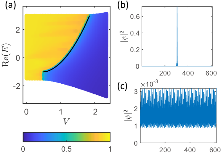
One convenient tool to identify localized states is the inverse participation ratio (IPR), defined as ${\rm IPR}(m)=\sum_{j}|\psi_{m,j}|^{4}$ [4, 26], where $m$ labels the eigenstates and $j$ labels lattice sites. Based on this, we can further introduce the fractal dimension of the wave function, $\Gamma=-\lim_{L\rightarrow\infty}\frac{\ln({\rm IPR})}{\ln L}$. One can show that for extended states $\Gamma\to 1$ while for localized states $\Gamma\to 0$. In Fig. 1(a) we plot the fractal dimension $\Gamma$ of each eigenstate as a function of $\real(E)$ and $V$. In addition, the black line represents the ME condition in Eq. (2). As expected, $\Gamma$ approaches zero and one for energies on opposite sides of the black line, respectively. This can be further confirmed by the spatial density profile of the respective eigenstates, see Fig. 1 (b)-(c). In other words, a given eigenstate is localized or extended depends on whether its eigenvalue satisfies $\log\absolutevalue{V}\leq G(\real(E))$ or $\log\absolutevalue{V}>G(\real(E))$ [64].

We can thus identify three distinct regimes in Fig. 1(a): for $V<V_{c1}$ ($V>V_{c2}$), the energy spectrum only contains extended (localized) eigenstates, while for $V_{c1}\leq V\leq V_{c2}$, an energy-dependent ME emerges. We will thus denote the regime $V_{c1}\leq V\leq V_{c2}$ as the intermediate phase, since both extended and localized states exist in the spectrum. More importantly, we find that an intermediate phase always exists when $t_{2}\neq 0$, and that the exact expressions for $V_{c1}$ and $V_{c2}$ are given by [64]

$\displaystyle\begin{aligned} V_{c1}&=\begin{cases}t_{2},&t_{2}\geq 1/4\\ \frac{1}{2}\quantity(\sqrt{1-4t_{2}}+1-2t_{2}),&0\leq t_{2}<1/4.\end{cases},\\ V_{c2}&=\frac{1}{2}\quantity(\sqrt{1+4t_{2}}+1+2t_{2}),\end{aligned}$

(5)

which are plotted in Fig. 2(a).

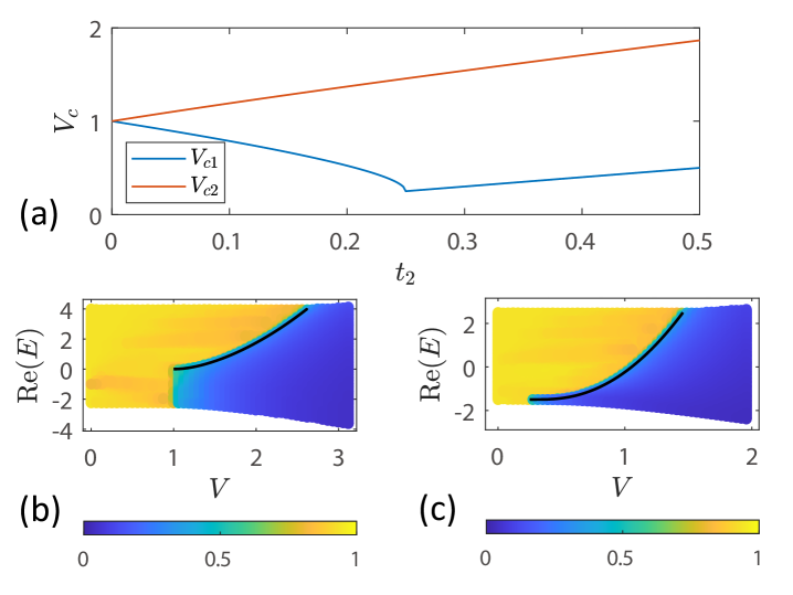
Interestingly, Fig. 2(a) shows a curious cusp in $V_{c1}$ at $t_{2}=1/4$, which implies that $t_{2}\leq 1/4$ and $t_{2}>1/4$ are two different regimes. This conjecture is confirmed in Fig. 2 (b)-(c), where we plot the ME for $t_{2}=1$ and $t_{2}=1/4$, respectively. We find that when $t_{2}>1/4$ [Fig. 2(b)], the number of localized states suddenly becomes finite as $V$ crosses $V_{c1}$. In contrast, when $t_{2}\leq 1/4$ [Fig. 2(c)], the number of the localized states increases continuously from zero as $V$ crosses $V_{c1}$. Therefore, we conclude that the structure of the ME is qualitatively different when $t_{2}\leq 1/4$ and $t_{2}>1/4$.

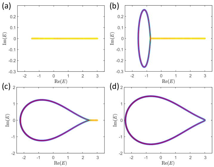
The $\mathcal{PT}$-symmetry breaking transition.— Apart from the metal-insulator transition described above, another interesting property of a $\mathcal{PT}$-symmetric non-Hermitian model is that this symmetry can be spontaneously broken when the non-Hermitian parameter $V$ exceeds a critical value. Moreover, it is known that this phase transition is accompanied by the transition from an entirely real spectrum to a complex one [57, 58, 59]. To demonstrate this property in our model, we keep $t_{2}=1/2$ and plot in Fig. 3 the spectrum for $V$ around $V_{c1}$ and $V_{c2}$, respectively. The results show that the analytical condition in Eq. (3) (shown as red lines in Fig. 3) correctly captures the spectrum of localized states. In addition, we can observe two different transitions. First, as $V$ increases beyond $V_{c1}$, complex energies start to emerge from a purely real spectrum, which is accompanied by the appearance of localized states. Second, as $V$ further increases beyond $V_{c2}$, the spectrum turns into a purely complex one and no extended states exist anymore. It is well known that in a $\mathcal{PT}$ symmetric model the spontaneous $\mathcal{PT}$ symmetry breaking underlies the real-complex transition of the spectrum. What is particularly interesting about our model is that the seemingly unrelated metal-insulator transition occurs simultaneously with the spontaneous $\mathcal{PT}$ symmetry breaking transition. In fact, we can prove this property rigorously, see Ref. [64].

Experimental realizations.— We now present a realistic experimental realization of the non-Hermitian $t_{1}$-$t_{2}$ model in Eq. (1) using a photonic lattice. Such photonic lattices have been routinely used to demonstrate Anderson localization of light [65, 66]. A schematic setup of our proposal is shown in Fig. 4(a). It is known that in the paraxial limit the propagation of classical light in a waveguide can be captured by a form of Maxwell equation that formally resembles the Schrödinger equation in quantum mechanics [67, 64]. If we further consider the limit in which the light is strongly confined by the waveguides, one can adopt the tight-binding approximation, and cast the continuum wave equation in the following form [67],

$\displaystyle i\derivative{\psi_{j}}{z}=\kappa_{j}\psi_{j}+\sum_{l\neq j}J_{j,l}\psi_{l}.$

(6)

Here the wave vector $\kappa_{j}$ is controlled by the refractive index contrast of the $j$th waveguide and the background medium, while the tunneling parameters $J_{j,l}$ are determined by the overlap between the evanescent tails of the eigenmodes in the $j$th and $l$th waveguides [67].

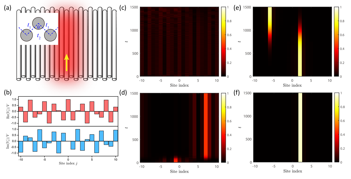
Our model in Eq. (1) can be realized in such a coupled waveguide system where the refractive index in the $j$th waveguide plays the role of potential $V_{j}$ and the temporal coordinate $t$ is replaced by the spatial coordinate $z$. In this work, we choose a system of $L=21$ coupled waveguides, see Fig. 4(a). In particular, it is possible to engineer the refractive indices of the waveguides so that their real and imaginary parts resemble the complex potential as plotted in Fig. 4(b). We further set $J_{j,j+1}=J_{j,j-1}=t_{1}$, $J_{j,j+2}=J_{j,j-2}=t_{2}$, and all other $J_{j,l}=0$. Further, the waveguides are arranged in a zigzag shape, so that the nearest neighbor coupling $t_{1}$ is larger than the next nearest neighbor coupling $t_{2}$. In this geometry the ratio $t_{2}/t_{1}$ can be tuned by the angle $\theta$ of the zigzag chain, see the inset of Fig. 4(a). Finally, periodic boundary conditions are preferred in the setup.

The localization property of this model can be probed by studying the light propagation in this coupled waveguide system. Here we choose to excite the waveguide at $j=0$ at $t=0$, and study how the light spreads out during the propagation. Effectively, we are evaluating

$$\ket{\psi(t)}=e^{-iHt}\ket{\psi_{0}}=\sum_{j}e^{-iE_{j}t}c_{j}\ket{E_{j}},$$

(7)

where $\ket{E_{j}}$ is the $j$th eigenstate of the Hamiltonian $H$ in Eq. (1) with an energy $E_{j}$, and $\quantity{c_{j}}$ are the superposition coefficients. The spatial extent of the time evolved state $\ket{\psi(t)}$ can be quantified by

$\displaystyle\bar{n}_{j}(t)\equiv\dfrac{\absolutevalue{\bra{w_{j}}\ket{\psi(t)}}^{2}}{\bra{\psi(t)}\ket{\psi(t)}},$

(8)

where $\ket{w_{j}}$ denotes the Wannier function localized within the $j$th waveguide.

We first consider the $V<V_{c1}$ regime, when all eigenstates in the system are extended. Consequently, we expect that almost all $\bar{n}_{j}(t)$ are nonzero at late times. In addition, because the spectrum is completely real, all the phase factors $e^{-iE_{j}t}$ satisfy $\absolutevalue{e^{-iE_{j}t}}=1$ at all times. As a result, all eigenstates will continue to contribute to the dynamics even when $t$ is large. Our expectations are verified by the results in Fig. 4(c), where we numerically plot $\bar{n}_{j}(t)$ when $V=V_{c1}-0.1$. In particular, we find that within a short time the initial excitation spreads out to other waveguides, and $\bar{n}_{j}(t)$ is almost evenly distributed among all waveguides.

In contrast, when the energy spectrum is complex, the time evolution operator $e^{-iHt}$ is dominated by the eigenstate whose energy eigenvalue has the largest imaginary part. For convenience, we denote this special eigenvalue as $E_{\text{amp}}$ and the corresponding eigenstate as $\ket{E_{\text{amp}}}$. In order to avoid numerical errors induced by the exponential amplifications in the presence of a complex spectrum, we further replace the original Hamiltonian $H$ by $H^{\prime}=H-i\gamma$ in our simulations, where $\gamma\equiv\imaginary(E_{\text{amp}})>0$. As a result, the state $\ket{E_{\text{amp}}}$ still dominates the quench dynamics, but its amplitude is preserved throughout the dynamics. In contrast, the amplitude of all the other eigenstates decays exponentially. Furthermore, since in this model all states with a complex energy eigenvalue are localized, we anticipate that the final state will be localized whenever the spectrum contains complex energies. In Fig. 4(d) we plot $\bar{n}_{j}(t)$ for $V=V_{c1}+0.3$, when the system is in the intermediate phase. We indeed find that the final state is localized. However, in contrast to the quench dynamics in a Hermitian system, the final state is not localized on the original waveguide at $j=0$, but collapses into the waveguide at $j=7$. Moreover, we find a curious ‘switching process’ during the dynamics. Specifically, the initial excitation in the $j=0$ waveguide almost instantly switches to a signal peaked at the $j=-1$ waveguide [64]. At around $t=100$, this signal switches again to one localized in the $j=7$ waveguide. During the entire quench dynamics, the maximum magnitude of $\bar{n}_{j}(t)$ reaches about $0.4$. We also find that the localization length of the final steady state is still quite large, as weak signals with $\bar{n}_{j}(t)\sim 0.2$ can still be seen in the neighboring waveguides at $j=4$ and $j=10$. The above observations show that localization in a non-Hermitian system is qualitatively different from that in Hermitian systems. In particular, the switching behavior can never occur in a Hermitian system.

In addition, in Fig. 4 (e)-(f) we plot $\bar{n}_{j}(t)$ for two different $V>V_{c2}$, when the system is in the localized phase. We find that the qualitative features of Fig. 4(d), especially the switching behavior, are preserved. For example, in Fig. 4(e) we find that the initial excitation in the $j=0$ waveguide quickly gives way to an excitation confined in the $j=2$ waveguide, before eventually collapses into the waveguide at $j=-6$. In comparison, in Fig. 4(f) we find that the initial excitation in the $j=0$ waveguide quickly collapses into the waveguide at $j=2$ and no additional switching happens afterwards. The main differences between the localized regime and the intermediate regime seem to be quantitative. For example, the localization length of the final steady state is now reduced to just one lattice site. Moreover, the peak value of $\bar{n}_{j}(t)$ now reaches about $0.8$ for Fig. 4(e) and about $0.9$ for Fig. 4(f), respectively. It turns out that the curious switching behavior of $\bar{n}_{j}(t)$ found in Fig. 4 (d)-(f) arise because there exist several eigenstates whose eigenvalues have similar imaginary parts. The switching is a result of the competitions between these eigenstates [64].

Discussion and Outlook.— Our work represents one of the first examples where the ME in the non-Hermitian quasiperiodic model cannot be directly inferred from its Hermitian counterpart. Indeed, while the exact ME in the Hermitian $t_{1}$-$t_{2}$ model is not yet known, we are able to determine the exact ME in our model. In addition, the method developed in this work is very general and can be applied to a wide class of quasiperiodic models. For example, an exact ME can still be obtained when $t_{2}$ is complex or when more remote hopping terms are included [64]. Our work thus not only proposes a realistic experimental scheme to demonstrate ME in a non-Hermitian quasiperiodic model, but also presents a general framework to study other 1D non-Hermitian quasiperiodic models. One important open question is the effect of interactions on the localization properties of this model [68, 69]. In particular, it is interesting to understand whether the interplay between interactions and the ME can lead to a many-body intermediate phase [70, 71, 72] in this non-Hermitian system.

Acknowledgements.— S.W. acknowledges support from the Research Grants Council of the Hong Kong Special Administrative Region, China (Project Nos. HKUST C6013-18G and CityU 11301820). X.L. acknowledges support from City University of Hong Kong (Project No. 9610428), the National Natural Science Foundation of China (Grant No. 11904305), as well as the Research Grants Council of the Hong Kong Special Administrative Region, China (Grant No. CityU 21304720).

References

- Anderson [1958] P. W. Anderson, Phys. Rev. 109, 1492 (1958).
- Abrahams et al. [1979] E. Abrahams, P. W. Anderson, D. C. Licciardello, and T. V. Ramakrishnan, Phys. Rev. Lett. 42, 673 (1979).
- Lee and Ramakrishnan [1985] P. A. Lee and T. V. Ramakrishnan, Rev. Mod. Phys. 57, 287 (1985).
- Evers and Mirlin [2008] F. Evers and A. D. Mirlin, Rev. Mod. Phys. 80, 1355 (2008).
- Schreiber et al. [2015] M. Schreiber, S. S. Hodgman, P. Bordia, H. P. Luschen, M. H. Fischer, R. Vosk, E. Altman, U. Schneider, and I. Bloch, Science 349, 842 (2015).
- Bordia et al. [2016] P. Bordia, H. P. Lüschen, S. S. Hodgman, M. Schreiber, I. Bloch, and U. Schneider, Phys. Rev. Lett. 116, 140401 (2016).
- y. Choi et al. [2016] J. y. Choi, S. Hild, J. Zeiher, P. Schauss, A. Rubio-Abadal, T. Yefsah, V. Khemani, D. A. Huse, I. Bloch, and C. Gross, Science 352, 1547 (2016).
- Lüschen et al. [2017a] H. P. Lüschen, P. Bordia, S. S. Hodgman, M. Schreiber, S. Sarkar, A. J. Daley, M. H. Fischer, E. Altman, I. Bloch, and U. Schneider, Phys. Rev. X 7, 011034 (2017a).
- Lüschen et al. [2017b] H. P. Lüschen, P. Bordia, S. Scherg, F. Alet, E. Altman, U. Schneider, and I. Bloch, Phys. Rev. Lett. 119, 260401 (2017b).
- Bordia et al. [2017] P. Bordia, H. Lüschen, S. Scherg, S. Gopalakrishnan, M. Knap, U. Schneider, and I. Bloch, Phys. Rev. X 7, 041047 (2017).
- Abanin et al. [2019] D. A. Abanin, E. Altman, I. Bloch, and M. Serbyn, Rev. Mod. Phys. 91, 021001 (2019).
- Soukoulis and Economou [1982] C. M. Soukoulis and E. N. Economou, Phys. Rev. Lett. 48, 1043 (1982).
- Das Sarma et al. [1986] S. Das Sarma, A. Kobayashi, and R. E. Prange, Phys. Rev. Lett. 56, 1280 (1986).
- Das Sarma et al. [1988] S. Das Sarma, S. He, and X. C. Xie, Phys. Rev. Lett. 61, 2144 (1988).
- Thouless [1988] D. J. Thouless, Phys. Rev. Lett. 61, 2141 (1988).
- Das Sarma et al. [1990] S. Das Sarma, S. He, and X. C. Xie, Phys. Rev. B 41, 5544 (1990).
- Biddle et al. [2009] J. Biddle, B. Wang, D. J. Priour, and S. Das Sarma, Phys. Rev. A 80, 021603 (2009).
- Biddle and Das Sarma [2010] J. Biddle and S. Das Sarma, Phys. Rev. Lett. 104, 070601 (2010).
- Biddle et al. [2011] J. Biddle, D. J. Priour, B. Wang, and S. Das Sarma, Phys. Rev. B 83, 075105 (2011).
- Ganeshan et al. [2015] S. Ganeshan, J. Pixley, and S. Das Sarma, Phys. Rev. Lett. 114, 146601 (2015).
- Deng et al. [2019] X. Deng, S. Ray, S. Sinha, G. Shlyapnikov, and L. Santos, Phys. Rev. Lett. 123, 025301 (2019).
- Li and Das Sarma [2020] X. Li and S. Das Sarma, Phys. Rev. B 101, 064203 (2020).
- Wang et al. [2020] Y. Wang, X. Xia, L. Zhang, H. Yao, S. Chen, J. You, Q. Zhou, and X.-J. Liu, Phys. Rev. Lett. 125, 196604 (2020).
- Xu et al. [2020] Z. Xu, H. Huangfu, Y. Zhang, and S. Chen, New J. Phys. 22, 013036 (2020).
- Roy et al. [2021] S. Roy, T. Mishra, B. Tanatar, and S. Basu, Phys. Rev. Lett. 126, 106803 (2021).
- Li et al. [2017] X. Li, X.-P. Li, and S. Das Sarma, Phys. Rev. B 96, 085119 (2017).
- Lüschen et al. [2018] H. P. Lüschen, S. Scherg, T. Kohlert, M. Schreiber, P. Bordia, X. Li, S. Das Sarma, and I. Bloch, Phys. Rev. Lett. 120, 160404 (2018).
- An et al. [2018] F. A. An, E. J. Meier, and B. Gadway, Phys. Rev. X 8, 031045 (2018).
- Kohlert et al. [2019] T. Kohlert, S. Scherg, X. Li, H. P. Lüschen, S. Das Sarma, I. Bloch, and M. Aidelsburger, Phys. Rev. Lett. 122, 170403 (2019).
- Goblot et al. [2020] V. Goblot, A. Štrkalj, N. Pernet, J. L. Lado, C. Dorow, A. Lemaître, L. L. Gratiet, A. Harouri, I. Sagnes, S. Ravets, A. Amo, J. Bloch, and O. Zilberberg, Nat. Phys. 16, 832 (2020).
- An et al. [2021] F. A. An, K. Padavić, E. J. Meier, S. Hegde, S. Ganeshan, J. Pixley, S. Vishveshwara, and B. Gadway, Phys. Rev. Lett. 126, 040603 (2021).
- Hatano and Nelson [1996] N. Hatano and D. R. Nelson, Phys. Rev. Lett. 77, 570 (1996).
- Hatano and Nelson [1997] N. Hatano and D. R. Nelson, Phys. Rev. B 56, 8651 (1997).
- Hatano and Nelson [1998] N. Hatano and D. R. Nelson, Phys. Rev. B 58, 8384 (1998).
- Feinberg and Zee [1999] J. Feinberg and A. Zee, Phys. Rev. E 59, 6433 (1999).
- Jazaeri and Satija [2001] A. Jazaeri and I. I. Satija, Phys. Rev. E 63, 036222 (2001).
- Molinari [2009] L. G. Molinari, J. Phys. A: Math. Theor. 42, 265204 (2009).
- Jović et al. [2012] D. M. Jović, C. Denz, and M. R. Belić, Opt. Lett. 37, 4455 (2012).
- Yuce [2014] C. Yuce, Phys. Lett. A 378, 2024 (2014).
- Liang et al. [2014] C. H. Liang, D. D. Scott, and Y. N. Joglekar, Phys. Rev. A 89, 030102 (2014).
- Mejía-Cortés and Molina [2015] C. Mejía-Cortés and M. I. Molina, Phys. Rev. A 91, 033815 (2015).
- Amir et al. [2016] A. Amir, N. Hatano, and D. R. Nelson, Phys. Rev. E 93, 042310 (2016).
- Harter et al. [2016] A. K. Harter, T. E. Lee, and Y. N. Joglekar, Phys. Rev. A 93, 062101 (2016).
- Longhi [2019a] S. Longhi, Phys. Rev. Lett. 122, 237601 (2019a).
- Tzortzakakis et al. [2020] A. F. Tzortzakakis, K. G. Makris, and E. N. Economou, Phys. Rev. B 101, 014202 (2020).
- Huang and Shklovskii [2020] Y. Huang and B. I. Shklovskii, Phys. Rev. B 101, 014204 (2020).
- Zeng et al. [2020] Q.-B. Zeng, Y.-B. Yang, and Y. Xu, Phys. Rev. B 101, 020201 (2020).
- Xu and Chen [2021] Z. Xu and S. Chen, Phys. Rev. A 103, 043325 (2021).
- Zeng et al. [2017] Q.-B. Zeng, S. Chen, and R. Lü, Phys. Rev. A 95, 062118 (2017).
- Longhi [2019b] S. Longhi, Phys. Rev. B 100, 125157 (2019b).
- Liu et al. [2020a] Y. Liu, X.-P. Jiang, J. Cao, and S. Chen, Phys. Rev. B 101, 174205 (2020a).
- Liu et al. [2020b] T. Liu, H. Guo, Y. Pu, and S. Longhi, Phys. Rev. B 102, 024205 (2020b).
- Zeng and Xu [2020] Q.-B. Zeng and Y. Xu, Phys. Rev. Research 2, 033052 (2020).
- Liu et al. [2021] Y. Liu, Y. Wang, X.-J. Liu, Q. Zhou, and S. Chen, Phys. Rev. B 103, 014203 (2021).
- Longhi [2021] S. Longhi, Phys. Rev. B 103, 144202 (2021).
- Liu et al. [2020c] Y. Liu, Y. Wang, Z. Zheng, and S. Chen, arXiv:2012.10029 [cond-mat.dis-nn] (2020c).
- Bender and Boettcher [1998] C. M. Bender and S. Boettcher, Phys. Rev. Lett. 80, 5243 (1998).
- Bender [2007] C. M. Bender, Rep. Progr. Phys. 70, 947 (2007).
- El-Ganainy et al. [2018] R. El-Ganainy, K. G. Makris, M. Khajavikhan, Z. H. Musslimani, S. Rotter, and D. N. Christodoulides, Nat. Phys. 14, 11 (2018).
- Sarnak [1982] P. Sarnak, Comm. Math. Phys. 84, 377 (1982).
- Kohmoto [1983] M. Kohmoto, Phys. Rev. Lett. 51, 1198 (1983).
- Wang et al. [2016] Y. Wang, Y. Wang, and S. Chen, Eur. Phys. J. B 89, 254 (2016).
- Note [1] Note that the energy spectrum is guaranteed to be real at the ME.
- [64] See Supplemental Material for additional details on the ME and the experimental protocol.
- Schwartz et al. [2007] T. Schwartz, G. Bartal, S. Fishman, and M. Segev, Nature 446, 52 (2007).
- Lahini et al. [2008] Y. Lahini, A. Avidan, F. Pozzi, M. Sorel, R. Morandotti, D. N. Christodoulides, and Y. Silberberg, Phys. Rev. Lett. 100, 013906 (2008).
- Ozawa et al. [2019] T. Ozawa, H. M. Price, A. Amo, N. Goldman, M. Hafezi, L. Lu, M. C. Rechtsman, D. Schuster, J. Simon, O. Zilberberg, and I. Carusotto, Rev. Mod. Phys. 91, 015006 (2019).
- Hamazaki et al. [2019] R. Hamazaki, K. Kawabata, and M. Ueda, Phys. Rev. Lett. 123, 090603 (2019).
- Zhai et al. [2020] L.-J. Zhai, S. Yin, and G.-Y. Huang, Phys. Rev. B 102, 064206 (2020).
- Hsu et al. [2018] Y.-T. Hsu, X. Li, D.-L. Deng, and S. Das Sarma, Phys. Rev. Lett. 121, 245701 (2018).
- Xu et al. [2019] S. Xu, X. Li, Y.-T. Hsu, B. Swingle, and S. Das Sarma, Phys. Rev. Research 1, 032039 (2019).
- Wang et al. [2021] Y. Wang, C. Cheng, X.-J. Liu, and D. Yu, Phys. Rev. Lett. 126, 080602 (2021).