A New Frequency-Luminosity Relation for Long GRBs?
Abstract
We have studied power density spectra (PDS) of 206 long Gamma-Ray Bursts (GRBs). We fitted the PDS with a simple power-law and extracted the exponent of the power-law () and the noise-crossing threshold frequency (). We find that the distribution of the extracted peaks around and that of around 1 Hz. In addition, based on a sub-set of 58 bursts with known redshifts, we show that the redshift-corrected threshold frequency is positively correlated with the isotropic peak luminosity. The correlation coefficient is .
keywords:
gamma-ray bursts1 Introduction
Gamma-ray Bursts (GRBs) show very complicated time profiles and, despite extensive investigations, are still not fully understood. The Fourier power density spectrum (PDS) of GRBs, on the other hand, seem to show relatively simple behavior. Giblin et al. (1998) found that a typical PDS shows a low-frequency power-law component and a high-frequency flat component (usually associated with Poisson noise). Beloborodov et al. (1998, 2000) considered each GRB as a realization of some common stochastic process and showed that when averaged over many bursts the resulting PDS exhibits a power-law behavior with an exponent of -1.67, which the authors note is consistent with the -5/3 Kolmogorov spectral index expected from processes involving turbulent flow. In addition, they claim that there is a break in the averaged PDS at 1 Hz. The authors were not in a position to correct their sample for the time dilation due to the cosmological redshifts.
Lazzati (2002) analyzed GRB power spectra by dividing them into six luminosity bins using the variability-luminosity correlation (Fenimore & Ramirez-Ruiz, 2000; Reichart et al., 2001; Guidorzi, 2005; Guidorzi et al., 2005, 2006; Li & Paczyński, 2006; Rizzuto et al., 2007). The PDS was averaged in each bin after correcting for pseudo-redshifts obtained through the variability-luminosity relation (Fenimore & Ramirez-Ruiz, 2000). Lazzati (2002) showed that the dominant frequency () of the PDS is strongly correlated with the variability parameter obtained by taking a modified variance of the de-trended light curve (Fenimore & Ramirez-Ruiz, 2000). Here is obtained by finding the maximum of the function (see Lazzati (2002) for more details). The author further states that the red-noise component of the averaged PDS for the six luminosity bins is well described by a broken power-law function with a low-frequency slope of -2/3 and high-frequency slope of -2. In this case, the break frequency is a function of both luminosity and the variability parameter.
Borgonovo et al. (2007) did a similar analysis of power spectra but used measured redshift information to correct for time dilation effects before averaging. The burst sample was subdivided into two populations based on the calculated values of the autocorrelation function. After averaging, the PDS of one population shows a power-law index of -2.0 (consistent with the spectral index expected of Brownian motion) and the PDS of the other population is characterized by a low-frequency exponentially decaying component and a high-frequency power-law component with an index of -1.6 (which again is consistent with the -5/3 Kolmogorov spectral index).
Most of the previous work on power density spectra of GRBs has been based on observations with the Burst and Transient Source Experiment (BATSE) on the Compton Gamma Ray Observatory (Giblin et al., 1998; Beloborodov et al., 1998, 2000; Lazzati, 2002; Borgonovo et al., 2007) where a relatively modest amount of redshift information is available. The launch of the satellite (Gehrels et al., 2004) ushered in a new era of GRB research. Due to its rapidly disseminated, arcsecond GRB positions, has enabled more subsequent redshift measurements of GRBs than ever before. The availability of redshift information enables the study of rest-frame properties of bursts and provides an opportunity for further exploration of correlations involving burst parameters such as luminosity and variability.
In this paper we present a study of Fourier power density spectra of 206 long bursts. Unlike previous work, we avoid averaging PDS of multiple bursts and examine them individually. We have developed a method to estimate the uncertainties in PDS for each burst. Then we extract PDS for all the GRBs in the sample and investigate the distribution of the extracted parameters. The structure of the paper is the following: In section 2 we discuss our methodology for extracting the PDS. In section 3, we present our results for a sample of 206 long bursts and investigate various correlations between the extracted parameters. In addition, we propose a new frequency-luminosity relation based on a sample of 58 GRBs with spectroscopically measured redshifts. In section 4, we discuss observational biases of our results. Finally, in section 5 we summarize our conclusions. In this work, we have adopted the standard values for the cosmological parameters: , and the Hubble constant is . Throughout this paper, the quoted uncertainties are at the 68% confidence level, unless noted otherwise.
2 Data Analysis
2.1 Light Curve Extraction
BAT is a highly sensitive, coded aperture instrument (Barthelmy et al., 2005). BAT uses the shadow pattern resulting from the coded mask to facilitate few arc-minute localization of gamma-ray sources. In order to generate background subtracted light curves, we used a process called mask weighting. The mask weighting assigns a ray-traced shadow value for each individual event, which then enables the user to calculate light curves or spectra.
We used the batmaskwtevt and batbinevt tasks in the BAT FTOOLS to generate mask weighted, background-subtracted light curves in the BAT energy range keV. The light curves that are generated have rates that are measured in counts per second per detector (). In addition, the above tools also generate uncertainties associated with the rates that are calculated by propagation of errors from raw counts (subject to Poissonian noise). For the BAT instrument one can potentially go down to the minimum time binning of 0.1 ms. However, in this work, we used 1-ms time binned light curves.
2.2 Fourier Analysis
We calculate the Fourier transform, , of each GRB light
curve, (measured in counts/sec/detector), using a standard
Fast Fourier Transform (FFT)111We used the FFT routine in
the IDL (Interactive Data Language) data analysis package.
http://www.ittvis.com/ProductServices/IDL.aspx
algorithm (Jenkins & Watts, 1969; Press, 2002). We used a time
segment of the burst light-curve where the total fluence is
accumulated (i.e. start and end times corresponding to burst T100
which is calculated by the battblocks task). The PDS of
each burst is calculated using . The power
spectra are not normalized nor are they averaged. In addition, we
have employed logarithmic binning for our power spectra.
This process of treating PDS individually is different from that of Beloborodov et al. (1998, 2000); Lazzati (2002) and Borgonovo et al. (2007), as they used some averaging process to obtain the slope of the red-noise component of the power spectra. The wide variety of light curves exhibited by GRBs is potentially indicative of different emission and scattering processes that eventually shape the observed light curves and therefore we have avoided averaging power spectra so as not to compromise this valuable information.
The uncertainties of the individual PDS are calculated as follows: For each burst, we simulate 100 light curves based on the original light curve () and its uncertainty (), i.e.
| (1) |
Here is a random number generated from a gaussian distribution with the mean equal to zero and the standard deviation equal to one. For each simulated light curve we calculate a PDS. Then we re-bin each PDS logarithmically. The uncertainties in the original PDS (obtained from the original light curve) are derived by taking the standard deviation of the 100 simulated PDS.
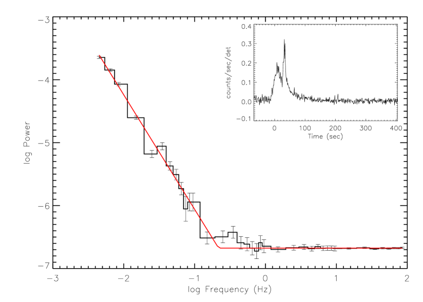
The power spectra for the GRBs in the sample are fitted with the function depicted in equation 2 (see figure 1 for a typical fit). This function consists of a power-law component (to fit the low-frequency “red noise” component) and a constant component (to fit the flat high-frequency “white noise” component).
| (2) |
Here is the threshold frequency where the red-noise component intersects the white-noise component of the power density spectrum, and is the white-noise power density.
3 Results
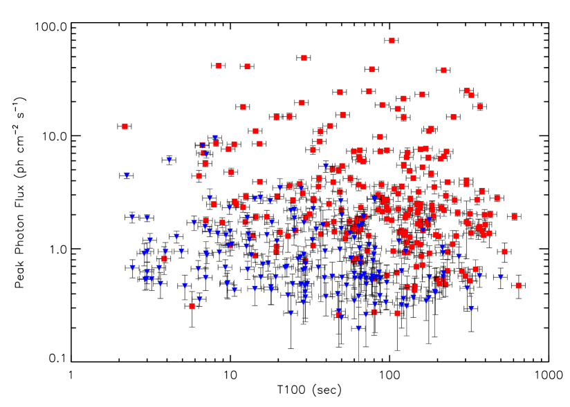
Out of 451 GRBs which triggered BAT from 2004 December 19 to 2009 December 31, we selected a sample of 226 long GRBs that show a significant red-noise component above the flat white-noise region. In figure 2, we represent the two samples (the sample with clear red noise component is shown in red boxes and the sample with no or weak red-noise component is shown in blue inverted triangles) in a peak-photon-flux versus T100-duration plot. For the most part, the bursts that do not show a clear red-noise component are generally either weak and/or short in duration.
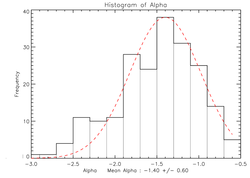
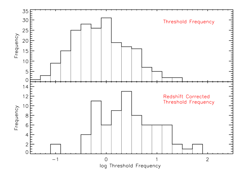
For the selected sample of 226 long GRBs we fitted the corresponding PDS with a simple power-law behavior given in equation 2, using the nonlinear least squares routine MPFIT (Markwardt, 2009). A typical fit is shown in figure 1. Out of the 226 GRBs in the sample, 20 bursts could not be fitted by a simple power-law. These GRBs were excluded from further analysis. For the final sample of 206 bursts, the distributions of the extracted slopes () and threshold frequencies () are shown in figure 3 and figure 4 respectively. The distribution of slopes (’s) has a Gaussian-like shape and peaks around -1.4 with of about 0.6. The distribution of threshold frequencies (’s) peaks around 1 Hz and also shows a broad distribution. The distribution of the redshift corrected (i.e. ), as depicted in the bottom panel of figure 4, shows a large dispersion and non-gaussian shape. In figure 5, we show a plot of and ; we see a very weak positive correlation () but we note at this stage of the analysis that has not been corrected for noise contamination nor has it been corrected for redshift.

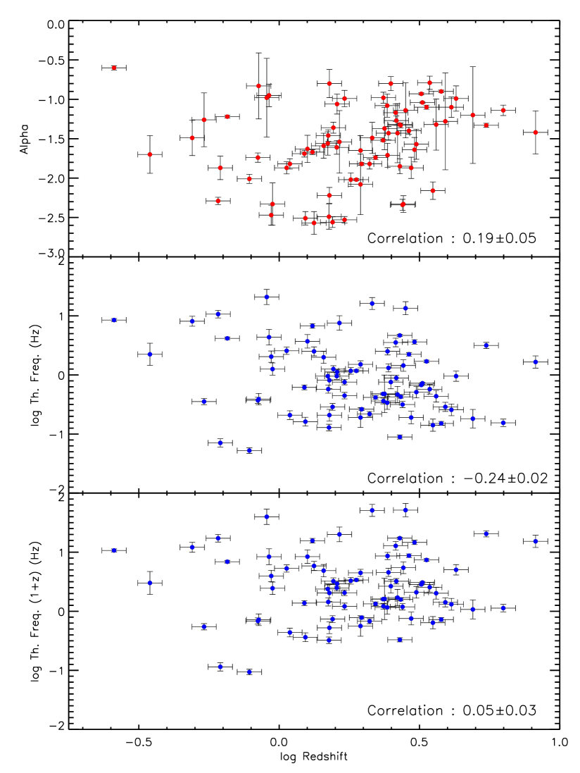
There are GRBs in our sample with measured redshifts (spectroscopic or otherwise). For this sub-sample it is interesting to see whether the extracted parameters are redshift dependent. Figure 6 shows (top panel), (middle panel), and the redshift-corrected (bottom panel) as a function of redshift. Very weak correlations are observed between and redshift and also between and redshift. However, no significant correlation is observed between and redshift.
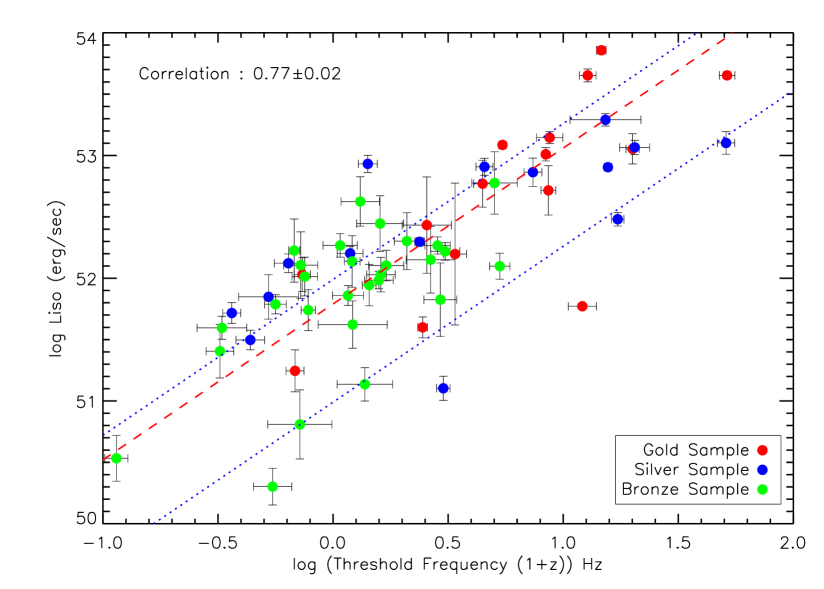
In Ukwatta et al. (2009) we proposed a correlation between the isotropic peak luminosity and the red-shift corrected based on 27 GRBs. To investigate this further with a larger sample we have selected a sample of 58 bursts with spectroscopically measured redshifts and good spectral information. For this sample, we have calculated isotropic peak luminosity as described in Ukwatta et al. (2010). Based on the availability of spectral information, we have divided the sample into three sub-samples: “Gold”, “Silver”, and “Bronze”. The “Gold” sample with 15 bursts have all Band spectral parameters measured (Band et al., 1993). In the “Silver” sample (15 bursts), the has been determined by fitting a cutoff power-law222 (CPL) to spectra. These 15 bursts do not have the high-energy spectral index, , measured, so we used the mean value of the BATSE distribution, which is (Kaneko et al., 2006; Sakamoto et al., 2009). The “Bronze” sample, with 28 bursts, does not have a measured . We have estimated it using the power-law index () of a simple power-law (PL) fit as described in Sakamoto et al. (2009). For these 28 bursts, the low-energy spectral index, , and the high-energy spectral index, , were not known, so we used the mean values of the BATSE and distribution, which are and respectively (Kaneko et al., 2006; Sakamoto et al., 2009).
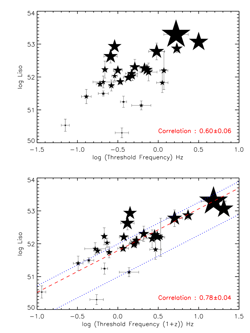
The isotropic luminosity as a function of the redshift-corrected threshold frequency is shown in figure 7. In the figure, the “Gold”, “Silver”, and “Bronze” samples are shown in red, blue, and green filled circles respectively. A clear positive correlation can be seen in the figure. The Pearson’s correlation coefficient is , where the uncertainty was obtained through a Monte Carlo simulation. The probability that the above correlation occurs due to random chance is . Our best-fit is shown as a red dashed line in figure 7 yielding the following relation between and :
| (3) |
To compensate for the large scatter in the plot, the uncertainties of the fit parameters are multiplied by a factor of where is the number of degrees of freedom. The blue dotted lines indicate the estimated 1 confidence level, which is obtained from the cumulative fraction of the residual distribution taken from 16% to 84%.
Our result for the slope in figure 7 is consistent with the value of obtained by Ukwatta et al. (2009) using 27 GRBs. This is encouraging because the results of Ukwatta et al. (2009) were obtained using non-mask-weighted event-by-event data instead of the mask-weighted data that we use in the current work. We also note that with the increase of the sample size by about a factor of two the correlation coefficient has increased from to . The correlation between frequency and luminosity is clearly intriguing but there remain observational biases which we address in a later section.
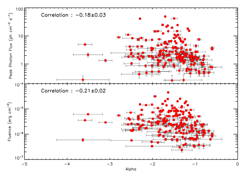
It has been reported previously (Beloborodov et al., 2000) that the PDS slope is correlated with the burst brightness. In order to check our sample for this effect, we display, in figure 8, the slope () against brightness indicators: the peak photon flux and the fluence. Very weak negative correlations are observed in both cases.
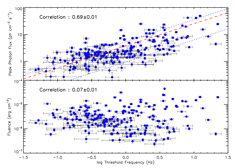
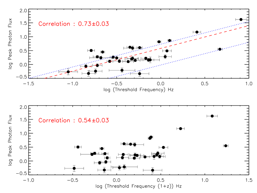
The other extracted parameter, the noise crossing threshold frequency () of the PDS, is also expected to depend on the brightness of the GRB. Presumably, the ‘red-noise’ component of the PDS comes primarily from the GRB but the flat ‘white-noise’ component can in principle arise from the Poisson noise (intensity fluctuations) associated with the GRB and the natural background in the field-of-view of the detector. For distant and/or intrinsically weak bursts, noise unrelated to the burst may dominate the observed white-noise component, thereby overwhelming the red-noise part of the signal. This, in turn, would make the extraction of the threshold frequency brightness-dependent. In figure 9 we plot the peak photon flux and the photon fluence as a function of the threshold frequency. The red dashed line in the top panel of figure 9 is the best fit, given by equation 4, and blue dotted lines indicate a confidence interval.
| (4) |
Indeed, a positive correlation can be seen between and the peak photon flux. However, no significant correlation is observed between and fluence. We discus this important matter further in the next section.
4 Discussion
It is conceivable that the proposed frequency-luminosity correlation is a direct result of the observed correlation between and the peak photon flux of the burst (see the top panel of figure 9). If this is the case, then for a statistically significant sample of bursts with similar apparent brightness, we should not see a correlation between and . In order to select a sample of GRBs with similar apparent brightness we plot in figure 10 the peak photon flux distribution for the sample of 58 bursts used to investigate the frequency-luminosity correlation in figure 7. We see from figure 10 that about half of the sample (28 GRBs) have a very similar peak photon flux (0.0 (peak photon flux) 0.5). For this subset of bursts we plotted their peak photon flux and as a function of and the results are shown in figure 11. In the top panel of figure 11, it is clear that there is a significant correlation between and with correlation coefficient of . This implies that the correlation observed in figure 7 ( - correlation) is not entirely due to the correlation seen in the top panel of figure 9 (peak photon flux correlation). We now correct the of this limited sample (with similar apparent brightness) for redshift to see its effect. Plotted in the bottom panel of figure 11 are the redshift corrected data. We note that the correlation strength increases to a value of , in part due to the natural correlation between redshift and .

In addition, we can approach the issue from the other direction, i.e., we select a subset of bursts with similar luminosity and ask the question whether the correlation between peak photon flux and comes from the proposed - correlation. In order to perform this test we selected a subset of bursts which have the roughly the same values (51.5 52.5) and plotted their peak photon flux as a function of . In figure 12, we show the peak photon flux as a function of (top panel) and the redshift corrected (bottom panel). There is clearly a strong correlation between the two parameters in both panels. It is interesting, however, that after the redshift correction, the correlation strength drops significantly. Accordingly, it would appear that the correlation between the peak photon flux and (top panel of figure 9) is not entirely due to the - correlation (figure 7). Since the spectral power is proportional to the square of the flux and the PDS follows a behavior (see figure 3), we expect to see a correlation between peak photon flux and . Hence, this correlation is in most part observational.
Now we turn to the question of the dependance of the extracted threshold frequency on the noise-level of the burst. The obvious question is how to determine the noise-level for each burst. One way of defining the noise-level is the following:
| (5) |
The detrending of the light curve (LC) can be done in a number of ways and we adopted the following method. We generated two light curves of the same burst with two bin sizes. In order to produce the coarser binned light curve, we chose a time bin size that resulted in at least 100 points in the burst duration (T100). The other light curve may have bin sizes that vary from 1 ms up to the coarser bin size. Clearly, with the different binning, the two light curves will have a different number of points. In order to properly detrend, we need to have the same number of points in the two light curves. We accomplish this by using a simple linear interpolation of the coarser binned light curve. The interpolated light curve is then subtracted from the finer binned light curve to generate the detrended light curve.
Using equation 5 we extract a noise level for each burst. However, the extracted noise-level depends on the bin size used in the detrending process. This aspect needs to be either removed or accounted for before the noise level of all the bursts can be treated on an equal footing.
The level of the flat white-noise region of the PDS does not depend on the bin size, i.e., for a given burst the white noise level is constant irrespective of the bin size, and for that matter so too are the extracted parameters and . In order to remove the bin size dependence in the extraction of the noise-level, we modify equation 5 as follows.
| (6) |
Here is the number of data points in the finely binned light curve. Our tests indicate that the results given by equation 6 do not depend on the time bin size of the light curve and provide a robust measure of the noise-level of a given burst.
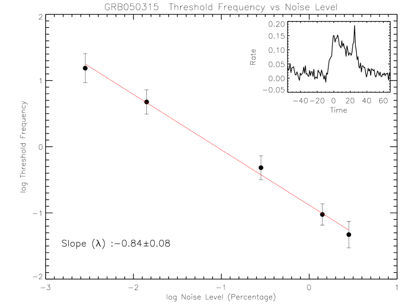
In order to further investigate the dependance of on the noise-level, we performed additional tests. We simulated different noise levels by adding increasing amounts of Gaussian noise to a burst light curve (in this case GRB 050315). Then we extracted values for each setting of the noise-level. Our results, the extracted frequency values versus the noise-level, are shown in figure 13 as a log-log plot. The threshold frequency does indeed depend on the noise-level. However, there is a linear relationship between the logarithmic values of the two quantities. This relation is important to know because it can be used to correct the extracted values to some nominal noise-level that is common to all bursts in the sample.
By performing the same test on the other bursts in our sample, we established that the relation between and the noise-level depends on the profile of the burst, i.e., the slope () of the log-log plot is different for each burst. Shown in the bottom panel of figure 14 is the distribution the slopes, , obtained for our sample of 58 bursts used in the - relation. Correspondingly, the noise-level () distribution is shown in the top panel of figure 14. This distribution shows a clear peak around the log value of -0.2 () while the distribution peaks around the value of -0.8.

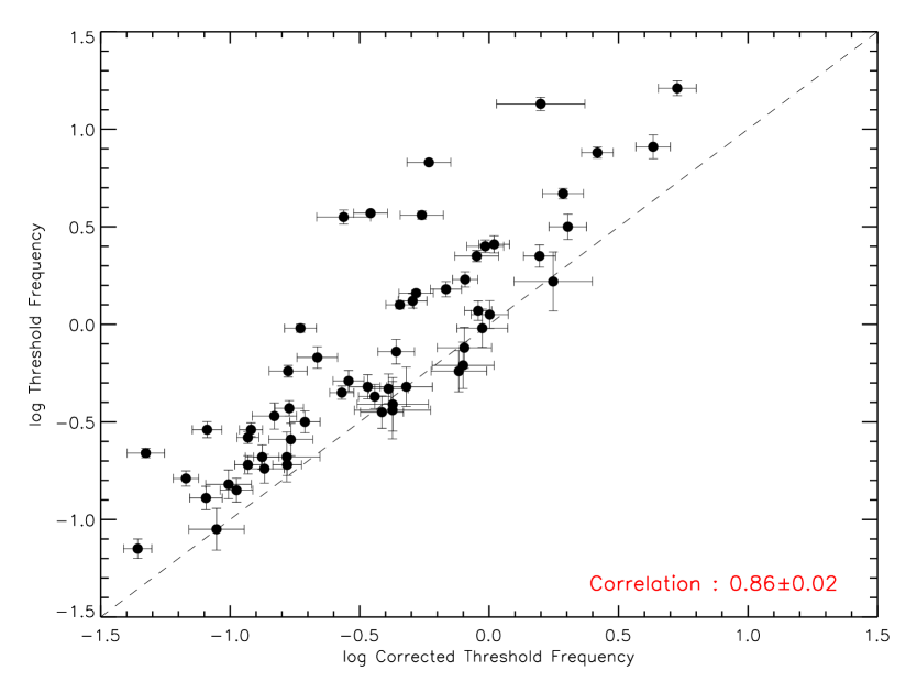
We are now in a position to treat all the bursts in our sample on an equal footing and test whether the - correlation, observed in figure 7, survives. The aim is to extract threshold frequencies which are consistent with a noise-level that is common to all the bursts in our sample. In order to accomplish this, we choose an arbitrary noise level of (see figure 13) and use the following relation to extract a corrected for each burst:
| (7) |
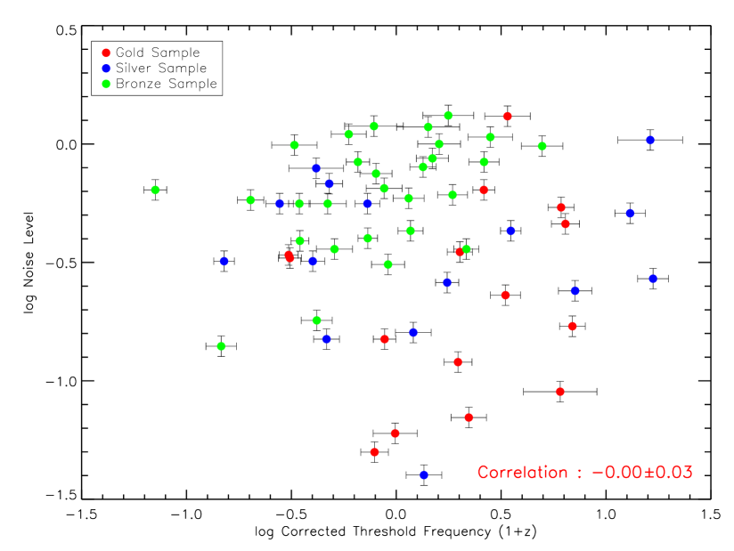
Here, is the extracted threshold frequency for a given burst, is the noise-level slope corresponding to the same burst and is the burst noise-level determined by equation 6. The correction procedure is repeated for each burst in our sample. To gauge the size of the correction, we plot in figure 15 (in a log-log scale) the corrected values versus the uncorrected . We note that there is a strong correlation between the two parameters. This is a reflection of the clustering of the and seen in figure 14. We also plotted the NL as a function of the noise-corrected, redshift-corrected in figure 16. There is no correlation between these two parameters, thus giving us confidence in the noise correction procedure.
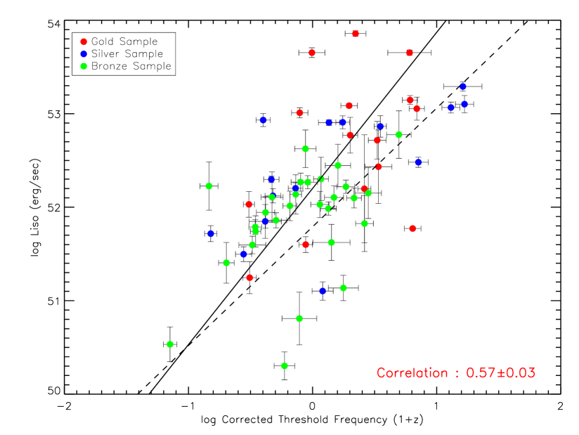
We show in figure 17 the noise-corrected threshold frequency - luminosity relation. As is evident, the relation survives the noise correction albeit with a somewhat smaller correlation coefficient of . Various correlation coefficients of the relation are shown in Table 1, where the uncertainties were obtained through a Monte Carlo simulation. The null probability that the correlation occurs due to random chance is also given for each coefficient type.
| Coefficient Type | Correlation Coefficient | Null Probability |
|---|---|---|
| Pearson’s | 0.570.03 | |
| Spearman’s | 0.580.04 | |
| Kendall’s | 0.430.03 |
The new best-fit is shown as a solid line in figure 17 yielding the following relation between and :
| (8) |
The uncertainties in the fitted parameters are expressed with the factor of .
5 Conclusion
In this paper we have analyzed PDS of 206 GRBs. We fitted each PDS with a simple power-law and determined the red-noise exponent and the threshold frequency where white noise begins. For a subset of GRBs, we extracted a frequency-luminosity relationship. For this sample, we treated all bursts on an equal footing by determining a common noise level, thereby minimizing the potential observational biases. We summarize the main results of our analysis as follows:
-
•
The distribution of the extracted (slope of the red-noise component) values peaks around -1.4 and that of around 1 Hz.
-
•
The dispersion in the distribution of is large and so the Kolmogorov index of -5/3 is accommodated by our analysis.
-
•
The distribution of the redshift-corrected threshold frequency shows a large dispersion and is non-gaussian in shape.
-
•
Evidence is presented for a possible frequency-luminosity relationship, i.e., the redshift-corrected is correlated with the isotropic luminosity. The correlation coefficient is and the best-fit power-law has an index of . We appreciate that in reality there may be complicated underlying interrelationships involving peak photon flux, , and redshift and therefore the evidence for the frequency-luminosity relation should be considered tentative.
-
•
The proposed frequency-luminosity correlation, if confirmed, may serve to provide a measure of the intrinsic variability observed in GRBs.
Acknowledgments
We thank the anonymous referee for comments and suggestions that significantly improved the paper. We also thank T. Sakamoto and C. Guidorzi for useful discussions. The NASA grant NNX08AR44A provided partial support for this work and is gratefully acknowledged.
References
- Band et al. (1993) Band, D., et al. 1993, ApJ., 413, 281
- Barthelmy et al. (2005) Barthelmy, S. D., et al. 2005, Space Science Reviews, 120, 143
- Beloborodov et al. (1998) Beloborodov, A. M., Stern, B. E., & Svensson, R. 1998, Self-Similar Temporal Behavior of Gamma-Ray Bursts, ApJ. Lett., 508, L25
- Beloborodov et al. (2000) Beloborodov, A. M., Stern, B. E., & Svensson, R. 2000, Power Density Spectra of Gamma-Ray Bursts, ApJ., 535, 158
- Borgonovo et al. (2007) Borgonovo, L., Frontera, F., Guidorzi, C., Montanari, E., Vetere, L., & Soffitta, P. 2007, On the temporal variability classes found in long gamma-ray bursts with known redshift, A.& A., 465, 765
- Fenimore & Ramirez-Ruiz (2000) Fenimore, E. E., & Ramirez-Ruiz, E. 2000, arXiv:astro-ph/0004176
- Gehrels et al. (2004) Gehrels, N., et al. 2004, ApJ., 611, 1005
- Giblin et al. (1998) Giblin, T. W., Kouveliotou, C., & van Paradijs, J. 1998, Power spectra of BATSE GRB time profiles, Gamma-Ray Bursts, 4th Hunstville Symposium, 428, 241
- Guidorzi (2005) Guidorzi, C. 2005, MNRAS, 364, 163
- Guidorzi et al. (2005) Guidorzi, C., Frontera, F., Montanari, E., Rossi, F., Amati, L., Gomboc, A., Hurley, K., & Mundell, C. G. 2005, MNRAS, 363, 315
- Guidorzi et al. (2006) Guidorzi, C., Frontera, F., Montanari, E., Rossi, F., Amati, L., Gomboc, A., & Mundell, C. G. 2006, MNRAS, 371, 843
- Jenkins & Watts (1969) Jenkins, G. M., & Watts, D. G. 1969, Holden-Day Series in Time Series Analysis, London: Holden-Day, 1969
- Kaneko et al. (2006) Kaneko, Y., Preece, R. D., Briggs, M. S., Paciesas, W. S., Meegan, C. A., & Band, D. L. 2006, ApJ. Supp., 166, 298
- Lazzati (2002) Lazzati, D. 2002, The role of photon scattering in shaping the light curves and spectra of gamma-ray bursts, MNRAS, 337, 1426
- Li & Paczyński (2006) Li, L.-X., & Paczyński, B. 2006, MNRAS, 366, 219
- Markwardt (2009) Markwardt, C. B. 2009, Astronomical Society of the Pacific Conference Series, 411, 251
- Morsony et al. (2010) Morsony, B. J., Lazzati, D., & Begelman, M. C. 2010, arXiv:1002.0361
- Press (2002) Press, W. H. 2002, Numerical recipes in C++ : the art of scientific computing by William H. Press. xxviii, 1,002 p. : ill. ; 26 cm. Includes bibliographical references and index. ISBN : 0521750334
- Reichart et al. (2001) Reichart, D. E., Lamb, D. Q., Fenimore, E. E., Ramirez-Ruiz, E., Cline, T. L., & Hurley, K. 2001, ApJ., 552, 57
- Rizzuto et al. (2007) Rizzuto, D., et al. 2007, MNRAS, 379, 619
- Sakamoto et al. (2009) Sakamoto, T., et al. 2009, ApJ., 693, 922
- Ukwatta et al. (2009) Ukwatta, T. N., et al. 2009, arXiv:0906.3193
- Ukwatta et al. (2010) Ukwatta, T. N., et al. 2010, ApJ., 711, 1073