A New Hybrid Automaton Framework with Partial Differential Equation Dynamics
Abstract
This paper presents the syntax and semantics of a novel type of hybrid automaton (HA) with partial differential equation (PDE) dynamic, partial differential hybrid automata (PDHA). In PDHA, we add a spatial domain and harness a mathematic conception, partition, to help us formally define the spatial relations. While classically the dynamics of HA are described by ordinary differential equations (ODEs) and differential inclusions, PDHA is capable of describing the behavior of cyber-physical systems (CPS) with continuous dynamics that cannot be modelled using the canonical hybrid systems’ framework. For the purposes of analyzing PDHA, we propose another model called the discrete space partial differential hybrid automata (DSPDHA) which handles discrete spatial domains using finite difference methods (FDM) and this simple and intuitive approach reduces the PDHA into HA with ODE systems. We conclude with two illustrative examples in order to exhibit the nature of PDHA and DSPDHA.
keywords:
Hybrid Automata, Cyber-Physical Systems, Partial Differential Equations1 Introduction
Cyber-Physical Systems have the potential to revolutionize the development of technology worldwide, and in recent years, numerous researchers and companies have invested significant time and money into ensuring that these systems will realize their economic and societal potential [1]. However, since CPS fundamentally integrate computational and physical processes, there are unique challenges in designing and analyzing these systems. In fact, the functional correctness of CPS relies deeply on the dynamics of their physical environment and the discrete control decisions of their computational units. Within hybrid systems, the framework of HA has demonstrated considerable utility in capturing the complex interactions between the discrete and continuous parts of a CPS. Additionally, it allows for a formal analysis of the safety and reliability of CPS [2]. However, this modelling framework has catered to systems with dynamics that can be described by ODEs, and hardly any attention has been paid to systems with dynamics described by PDEs [3].
Meanwhile, safety of certain CPS relies on reachable set/state estimation results that are based on Lyapunov functions analogous to stability [4, 5, 6, 7, 8, 9, 10] and reachability analysis of dynamical systems [11, 12], certainly have potentials to be further extended to safety verification. One can study the stability of switched systems, a switched system is composed of a family of continuous or discrete-time subsystems along with a switching rule governing the switching between the subsystems, with the help of the given switching rules described by a prescribed state space partitioning [13, 14, 15] or some known constraints on switching sequence such as dwell time [16, 17] or average dwell time [18, 19] restrictions.
PDEs are accomplished at describing a wide range of phenomena such as fluid dynamics and quantum mechanics that cannot be adequately described by ODEs [20, 21, 22]. As an example, a typical application for PDEs is the modelling of congestion in highway networks [23], and one popular model for highway control is the Lighthill-Whitham-Richards (LWR) model [24, 25]. Within this context, the PDEs evolve in an infinite dimensional space and must be discretized for computational purposes. In our approach, we seek to extend the existing framework from ordinary differential equations to partial differential equations. However, this extension is non-trivial since the internal structure of HA with PDEs is inherently more complicated due to the fact that switching and jump conditions cannot be easily specified. An in-depth discussion of these complexities, along with a discussion of three types of switching conditions, can be found in the following paper by [26].
While the hybrid automata theory for ordinary differential equations (ODEs) has been extensively studied (e.g., see [27, 28]), the theory for partial differential equations (PDEs) is still in the stage of case study [29, 30, 31, 32]. The main challenges in this area can be attributed to two factors:
-
(1)
The dynamics of automata involve switching due to known constraints, which gives rise to the so-called free boundary problem. This problem entails tracking the interface between different stages. In the context of PDEs, analyzing and numerically solving the free boundary is highly challenging (e.g., see [33, 34, 35, 36, 37, 38, 39]).
-
(2)
Unlike ODEs, PDEs incorporate various types of boundary conditions. Determining suitable boundary conditions for the partition is a complex task that poses numerical challenges.
Therefore, in this article, we present a novel approach to address the hybrid automata problem with partial differential modelling. Our approach aims to reduce the PDE problem to a manageable ODE hybrid automaton by employing a standard numerical discretization technique known as the finite difference method.
2 Running Examples
Before illustrating the main ideas of our framework, we use two running examples throughout the paper. The components of these running examples are depicted in Figures 1 and 2. The heater model consists of three devices: (i) a rod that can be heated using a gas burner from anywhere, (ii) a long gas burner that can be turned on or off partially in any region, and (iii) a thermometer that monitors the temperature of the rod at every location and periodically issues signals when the temperature of the rod is above or below certain a threshold. The goal is to design a control policy that maintains the temperature of the rod within a given range.
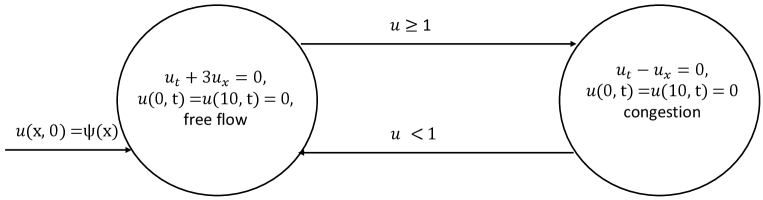
The second model we consider is a traffic model that was originally proposed in [26]. The system consists of a highway segment in which vehicles flow in and out. Vehicles maintain a high speed when the traffic flow density is below a given critical density and when the density exceeds the critical threshold, the speed of the traffic wave and the overall flow capacity decrease.
2.1 Heater Model
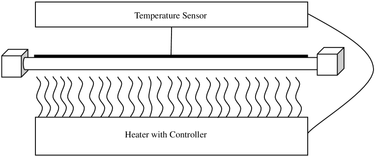
We first describe the behavior of the temperature of the rod. When the gas burner is OFF, the temperature of the rod, denoted by the variable , decreases according to the following PDE: where is the thermal diffusivity. The thermal diffusivity measures the rate of heat transfer of a material from the hot side to the cold side. The boundary conditions are and , which denote that at the location and the temperature is fixed to be , and heat is absorbed. denotes the space coordinate and denotes time. This law, however, is only true when the temperature of the corresponding position on the rod is greater than 0.7. When the heater is OFF, and the temperature of a position on the rod is below 0.4, the heater at that position will be turned on. The heater function is defined as . The maximum of the heater function appears at and the minimum is at . During the heater ON mode, the temperature is governed by the equation where is the function defined above. As one can see from the description of the evolution of the temperature, the system is not purely continuous. The system can switch from one mode to another by turning the heater on and off at a specific location on the rod.
2.2 Traffic Flow Model

The traffic model describes how traffic conditions may behave on a given highway. In free flow mode, which means the density is less than a specified critical density , the density function is given by the following equation , where is always a positive number and denotes that the traffic flow propagates forward. However, if the traffic density achieves , the system transitions into a high-density congestion mode. In this mode, the governing equation is described by , where is always a negative number and denotes that traffic congestion always moves backwards and propagates upstream. As an example, one of the causes of congestion may be a result of merging slow and fast-moving traffic, resulting in a high-density traffic flow. In this model, we can frequently switch between a free-flowing mode and a congestion mode, and as a result, a more powerful hybrid framework is needed to formalize these kinds of system behavior.
Additionally, the two models we have outlined present a mixture of space and time variables and are therefore quite complicated. In the following sections, we present a framework that is able to capture such a mixture of discrete and continuous behaviors, where PDEs describe the temporal and spatial dynamics.
3 Partial Differential Hybrid Automata
3.1 Transitions, Trajectories and Executions
Due to the properties of PDEs, the switching structure is more involved than in the case of ODEs [26]. One highway congestion alleviation model in [23] considers connected segments, where each segment is governed by an independent LWR PDE [24] with one side boundary condition. Each segment affects the boundary condition of the preceding segment and serves as an input function to the PDE. Additionally, the system is allowed to switch to another mode that incorporates a speed limit. One control approach for transport systems [40] proposes rules for switching based on criteria of minimizing a cost function. We outline two specific structures that are of interest to our framework:
-
1.
Switching PDEs in time on the full spatial domain. This situation is portrayed in Figure 3 (left) and is the PDE counterpart of hybrid systems as defined in [41], where a game theory approach is used to determine when mode switching occurs. Boundary condition switching has been investigated in highway traffic applications in [42]. PDE switching in time appears in [40] and in [23] and the latter one contains switching between modes in each highway segment.
-
2.
Switching PDEs on subsets of the time-space domain. This is illustrated in Figure 3 (right). Examples include the LWR PDE, in [23] where each highway segment is coupled with a boundary condition at the starting point of itself. This also appears in [24], where the LWR with triangular flux function can be decomposed into two modes (two one-dimensional wave equations) resulting in a partition of the space in regions with forward travelling waves, and regions with backward travelling waves.
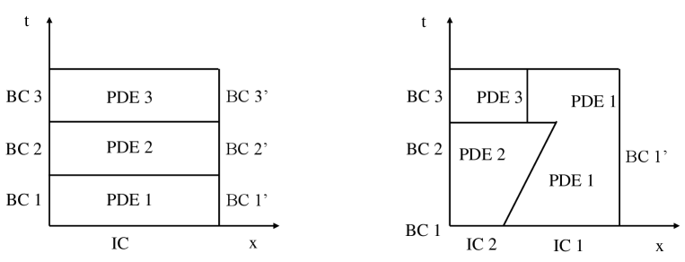
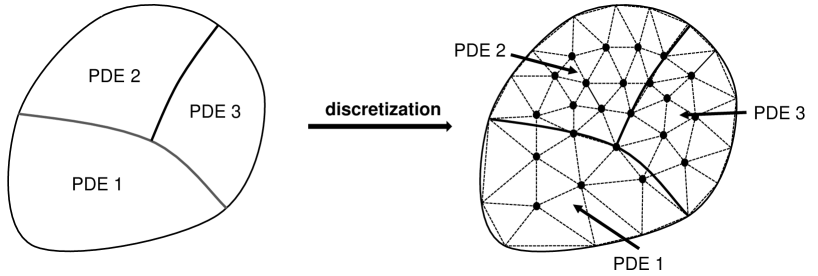
In order to describe the partial domain switching case in Figure 3 (right), it is useful to partition the whole domain into several parts and assign each one a corresponding mode. One possible solution is to use the union of disjoint domains to represent the region governed by specific modes. For example, the heat equation with (mode 1) and without heat source can cover domain . The equation with external source (mode 2) occupies domain .
Based on this idea, the main challenge is how to formalize the particular structure of the domain occupying behavior. One approach is to associate the union operator with the modes of the system. Thus, the system mode can be described as a composition of multiple modes , where each mode specifies the domain it occupies. Like in , when and in , when , where is the region occupied by . Thus, the space domain is composed of and .
This embodies our approach to represent the multiple mode occupation phenomenon, and we refer to the multiple mode occupation as the changing behavior of . The remaining challenge is to how to describe the moving behavior of the modes. This can be realized by changing , together with its boundary condition. As the system evolves, points satisfying a given condition will be moved from one mode to another and cause to grow or shrink. We call this point’s moving behavior a trajectory. The evolution of is not easily depicted. It can be a function of time or a function of several other complicated variables. Additionally, it might be impossible to predict switching behavior due to the complexity exhibited by the PDE’s solution.
Based on the ideas discussed above, the concept of spatial control mode is given below.
Definition 1 (Spatial Control Mode).
Let be a space domain. Let be a finite set of control modes, where each mode is denoted as . A space control mode consists of a union of control modes, where each mode covers part of the space domain . The spatial control mode is denoted by where and the region mode covers is denoted by and is a set map . Additionally, , where .
Now, according to our definition, is a subset of and not just an element in . We want to emphasize that the system could occupy several control modes simultaneously, rather than stay at a single mode as defined in classical hybrid automata. In order to accommodate and and for the purposes of formalizing domain division, we rely on partition defined in Definition 2. One can see that is a partition of domain since each is nonempty, and for . For convenience, we denote a specific partition of consisting of s and denote a set containing all possible partitions of domain .
Definition 2 (Partition [43]).
A partition of a set is a set of nonempty subsets of such that every element in is in exactly one of these subsets. Equivalently, a family of sets is a partition of if and only if all the following conditions hold:
-
1.
The family does not contain the empty set (that is ).
-
2.
The union of the sets in is equal to (that is ).
-
3.
The intersection of any two distinct sets in is empty (that is () ).
It is worth noting that the new PDE dynamic hybrid automaton needs a function to describe its state value. The additional spatial variable requires us to specify the values at different space locations while, in classical hybrid automata, the system only has finite values since the system only considers finite continuous state variables. The values of these state variables and discrete modes can be determined as long as the time is fixed, and the system is deterministic. In our model, for any time , we regard that the PDE solution lies in the state space . In other words, for any given , represents a real-valued trajectory.
After we obtain , and , the state can be defined now.
Definition 3 (State).
A state is a collection of variables that describes the current condition of a PDE dynamic system. It consists of a space control mode , a partition of a domain and a real function defined on .
| (1) |
In Figure 3 (left), each mode occupies the whole space domain and the system stays in only one mode. We have , . In Figure 3 (right), PDE 1 (mode 1) and PDE 2 (modes 2) occupy the whole domain , and at . It is worth stressing the differences between representing a state in PDE dynamic hybrid automata and classical hybrid automata. For discrete modes, the combination of and replaces the single and describes the space occupation behavior.
Bearing the above in mind, the next step is to formalize the flow function.
Definition 4 (Flow).
A flow for a PDE dynamic hybrid automaton is of the form which maps from one state to another as time evolves.
Similar to classical hybrid automata, PDE equations simulate the dynamics of the system. The flow consists of a piecewise PDE equation and the corresponding domain partition. A simple flow function for the heater example can be formally represented as
Definition 5 (Transition).
A transition in a PDE dynamic hybrid automaton is of the form which maps the current mode and partition to another. is a finite set of events.
Definition 6 (Reset).
A reset function for a PDE dynamic hybrid automaton is of the form which specifies how the value of changes when a transition takes place.
The ON mode, triggered by conditions defined in the set , for example (Figure 4), , then so that while the OFF mode happens when , we set , then .
3.2 Partial Differential Hybrid Automaton (PDHA)
With the above discussion in mind, we can now provide a formal definition of a partial differential hybrid automaton.
Definition 7 (Partial Differential Hybrid Automaton (PDHA)).
A partial differential hybrid automaton is a tuple where:
-
1.
is a set of finite s that represents control modes.
-
2.
is a finite set of events.
-
3.
is a space domain and .
-
4.
is a set of all partitions defined on domain .
-
5.
is a function space defined on domain and .
-
6.
is a set of initial states and .
-
7.
is a set of invariants defined for each mode .
-
8.
is a flow function and has the form :
where , is the continuous segment in , is the Laplacian, is the gradient, and is the domain covered by .
-
9.
is a transition map.
-
10.
is a set defining guard condition, .
-
11.
is a reset function.
In our framework, each mode contains only one PDE instead of a system of equations as in classical hybrid automata. Boundary conditions must not be violated and can be treated as a kind of invariant. They are imposed on the boundary of and act like constraints within the mode. Additionally, they are forced to be satisfied even during mode discrete transitions.


Revisiting the examples outlined at the very beginning, we construct two models to illustrate the idea of PDHA in Figures 1 and 2. In each model, the system is composed of two modes and each mode is governed by a PDE, the given boundary conditions, and the initial condition. In the heater model, we have .
The continuous trajectory is realized by moving a point satisfying a guard condition to another mode. In the heater model, a point in the mode ON where the temperature exceeds the threshold will be transferred to the mode OFF, meaning the heater located at this point is turned off while the other areas remain unchanged. At the same time, as the temperature at some points drops below some given bound, the heater at that location is turned on and the point at mode OFF will be moved to mode ON.
The same rule applies to the traffic model as well. The points in the free flow mode satisfying the guard condition will be moved to a congestion mode, and points in the congestion mode satisfying will be moved to the free flow mode.
4 Discrete Space Partial Differential Hybrid Automaton
In this section, we describe some core steps in deriving DSPDHA. First, we define a discretization scheme and use it to discretize a PDHA to construct its “discrete” model for analysis. Second, using this discretization scheme, we define a discrete PDHA that is related to the original PDHA via a “discretization relation” corresponding to the scheme .
4.1 Discretization Scheme and Discretization Relation
A discrete treatment of PDEs requires the use of new tools to realize the functions we need. One of the most widely used sets of methods is called finite difference methods (FDMs). Generally speaking, FDMs are a family of numerical approaches for solving differential equations by replacing them with an approximation using difference equations. Combining FDMs and PDHA produces the following definition:
Definition 8 (Discretization Scheme).
A discretization scheme is a numerical scheme to discretize a continuous partial differential equation into a set of algebraic equations (full-discretization scheme) or ordinary differential equations (semi-discretization scheme).
We present several schemes below to demonstrate how this technique approximates spatial derivatives.
Example 4.1 (Finite Difference Method Discretization Scheme).
A common example is shown for the heat equation using the central difference scheme:
| (2) |
where the scheme is based on a uniform mesh, is the grid size, , is a list of locations where the mesh points sit, and these points are the same ones defined in . Additionally, denotes the value at the position given time and the respective derivative is approximated using itself and the two adjacent values. The proof is based on using Taylor’s expansion with error .
After applying (2) and dropping the redundant part , the heat equation becomes
| (3) |
We replace by since the derivative with respect to space has been removed. Thus, is used to represent the time derivative at the grid point , and represents the input function valued at the same location.
Once the scheme has been chosen, the relation between our models can be described by the following definition.
Definition 9 (Discretization Relation).
If the model is obtained from the model via discretization scheme , we say that the model relates to the model via discretization scheme , which is denoted by: .
4.2 Discrete Space Partial Differential Hybrid Automaton
Using a discretization scheme, we obtain discrete models of the state, transition, flow and reset function of the original PHDA. These discrete models are defined below.
Definition 10 (Discrete Domain).
Let be a domain and , a discrete domain of is a set of distinct points obtained from by a discretization scheme : , and is the number of points. We say .
Example 4.2 (Discrete Domain of Heater Model).
Consider the heat equation defined on domain . One possible corresponding discrete domain is .
Definition 11 (Discrete Partition).
Let be a set of modes, is the set of all partitions on and . A discrete partition is a set of values, and each value is associated with a point . The set of all possible s is denoted by and .
In contrast to the continuous domain hybrid automaton which uses to describe the current mode that the system occupies, a discrete partition combines the two notations and simplifies the expression.
Example 4.3 (Discrete Partition of Heater Model).
Consider the model with OFF, ON and . Then , and can be expressed as .
Definition 12 (Discrete State).
A discrete state is an ordered pair where is a discrete partition on and is a list of real values. We denote the set of all possible s by and say where is the set of states defined in PDHA.
A discrete state gives the whole picture of the system by combining a discrete partition and state values.
Example 4.4 (Discrete State of Heater Model).
One discrete state can be in the form , where are the modes and the succeeding numbers are the temperatures at each node.
Everything listed above leads us to discrete flow.
Definition 13 (Discrete Flow).
Let be a flow function, is the set of discrete flow functions such that the spatial derivative of is approximated using . We say .
Example 4.5 (Discrete Flow of Heater Model).
Consider the heater example again,
The spatial derivative is approximated by a FDM centred difference scheme based on a uniform mesh of step size . We obtain a system of ODEs: In place of , we obtain an ODE system for , , :
where due to the boundary condition. We would like to remark that the convergence of FDM is due to the Lax–Richtmyer theorem [44].
Definition 14 (Discrete Transition).
A discrete transition of a DSPDHA is of the form which maps a current discrete partition to another. We say where is the transition defined in the original and is the discretization scheme.
Example 4.6 (Discrete Transition of heater model).
In order to illustrate the idea of a discrete transition, we make a simple modification of the previous example:
A transition to the mode ON at location and occurs because event takes place. Thus, we can write the transition function
| (4) |
where , , represents mode OFF and represents mode ON.
Definition 15 (Discrete Reset).
A discrete reset function of a DSPDHA is of the form which specifies how a value of changes to a new value when a transition takes place. We say where on the right is the reset function in original .
Definition 16 (Discrete Space Partial Differential Hybrid Automaton (DSPDHA)).
A discrete space partial differential hybrid automaton is a tuple where:
-
1.
is a set of finite modes;
-
2.
is a set of finite events;
-
3.
is a set of points;
-
4.
is a set of values defined on domain , ;
-
5.
is a set of discrete values defined on , ;
-
6.
is a set of initial states, ;
-
7.
is a set of invariants defined for each mode ;
-
8.
is a set of discrete flow functions and have the form :
(5) where denotes time derivative of ;
-
9.
is a transition function;
-
10.
is a set defining guard condition, ;
-
11.
is a reset function.
A key observation is if the discrete space partial differential hybrid automaton is obtained from a partial differential hybrid automaton through .
The DSPHDA provides us with a set of properties that can easily be formalized and stated. Additionally, similar concepts that appear in HA are outlined below.
Definition 17 (Hybrid Time Trajectory).
A hybrid time trajectory is a finite or infinite sequence of intervals of the real line, such that
-
1.
for ;
-
2.
if , then either , or ;
-
3.
for all , .
where are the time when discrete transition takes place.
Now that we have defined the syntax of DSPDHA, we define the semantics in terms of executions.
Definition 18 (Execution).
An execution of a DSPDHA is a collection satisfying
-
1.
Initial Condition: Init;
-
2.
Continuous Evolution: for all with , is a constant, is a solution to the ODEs (5) over and for all , ;
-
3.
Discrete Evolution: for all , .
An execution is called finite if is a finite sequence ending with a closed interval, infinite if is either an infinite sequence, or if , and Zeno if it is infinite but .
Definition 19 (Zeno Execution).
An execution is Zeno if
| (6) |
Here is called the Zeno time.
We use to denote the set of all executions of DSPDHA with initial condition , to denote the set of all finite executions, to denote the set of all infinite executions, and to denote the union of over all .
Definition 20 (Zeno Discrete Space Partial Differential Hybrid Automaton).
A discrete space partial differential hybrid automaton DPH is Zeno if there exists such that all executions in are Zeno.
| (7) |
Here is called the Zeno time.
The set of states reachable by a DSPDHA, , is defined as
| (8) |
where .
Definition 21 (Nonblocking).
A DSPDHA is called nonblocking if is nonempty at all .
Definition 22 (Deterministic).
A DSPDHA is called deterministic if contains at most one element for all .
More definitions about DSPDHA are similar to those in the classical HA theory, and we omit them here for the simplicity of the presentation.
4.3 Relation to Classical Hybrid Automaton
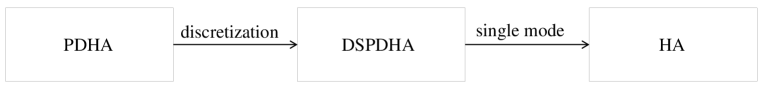
In this section, we explore the relations between classical hybrid automata, DSPDHA and PDHA. The central basis of introducing PDHA is extending HA with ODE dynamics to discretize PDE dynamics. To achieve this goal, some adjustments need to be made to accommodate the new framework within the classical hybrid automata scheme. It is our hope, that after these changes, the properties that hold for HA will hold for PDHA as well. This is the basis for the motivation to add an intermediate level (DSPDHA) lying between PDHA and HA, which captures the idea of PDHA and also stays close to classical HA. Using this framework, we make comparisons and illustrate useful results in the form of theorems.
In PDHA, we use space control modes and partitions to replace a discrete mode , a state function to replace state variables . The weakness of this scheme is determining executions and transitions because evolves continuously. DSPDHA overcomes these shortcomings by introducing a discrete state partition, which functions similarly to in HA. Along the same lines, a discrete flow function obtained from PDHA by FDM is essentially the same as a HA flow function. This allows us to assert some PDE system properties where we cannot otherwise reason with certainty due to a lack of information. We lay out several points below to illustrate how these connections are built.
-
(1)
Any DSPDHA is a HA if has identical elements. Based on the knowledge that elements in represent the modes where each location resides, identical elements indicate all the locations are assigned to the same modes and the system stays at a single mode. Therefore, the given DSPDHA is a HA. Thus, the general dynamical properties of HA, for instance, the existence, uniqueness, continuous dependence, reachability, stability and invariant sets follows. (See [45]). On the other, the DSPDHA inherits the physical feature (like diffusion) from the PDE model, which we demonstrate in the heat model below.
-
(2)
If the order of the time derivative of the PDE considered in a PDHA is , the number of points , in a discrete domain is equivalent to the size of flow functions in the corresponding DSPDHA. According to Definition 13, the discretization is made on each discrete point in . As a result, we have equations eventually.
-
(3)
If the order of the highest time derivative of a PDE is , then the PDE can be reduced to a system of PDEs with a order time derivative. We begin the proof by a change of variables. Let us replace the order time derivative of by and add a new equation to the system once the replacement is done. In the end, we obtain a system of equations in the form below.
(9) where the original equation is and is its time derivative. For example, we can deal with the wave equation .
-
(4)
If the order of time derivative of the PDE considered in a PDHA is and the number of points in discrete domain is , the size of flow functions in the corresponding DSPDHA is . Since determines the number of mesh points and each point is associated with an ODE ( order PDE after spatial discretization), equals the dimension of the system of ODEs which is the flow function.
Besides investigating the relation and distinction between models above, an interesting observation which occurs in classical hybrid automata are discontinuity issues, especially under PDE dynamics. [40] discusses the propagation of discontinuities when the system switches mode. They are numerous reasons why discontinuities occur. For the transport equation with a nonlinear flux function, there does not always exist a smooth solution, and a weak solution has to be constructed to handle a shock or rarefaction wave [46]. Jump discontinuities for hyperbolic system are discussed in [47].
The situation discussed in [40] is likely to happen if the discrete transition takes place in our framework. Consider a segment of road governed by a transport equation and the model is . Supposing the switching is triggered, and a new model is introduced, the latter model which involves fast wave speed will push the front flow to move fast, and the traffic will start to accumulate at the boundary of the road which directly leads to a discontinuity.
5 Experiments on Running Examples
The heater and traffic examples are formalized as DSPDHA and analyzed in this section. 111Code for the experiments is available at https://drive.google.com/drive/folders/1qnpwlU9WdVNjYm8lsZOjAqFIQhGhH0ME?usp=sharing
Heater Model.
As illustrated above, the first example is the bronze rod with two isolated ends. The heater provides heat to the rod and can be partially turned on and off at any time once the temperature reaches the given thresholds. For the input function, a linear increment function is considered with a maximum value appearing on the left and a minimum value appearing value on the right. The diagram of the model is in Figure 8.
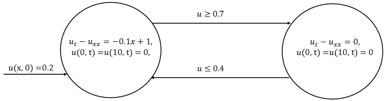
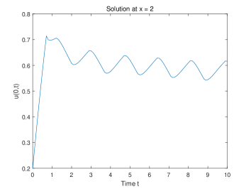
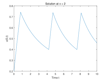
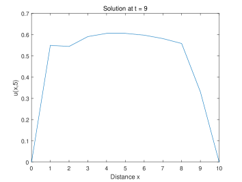
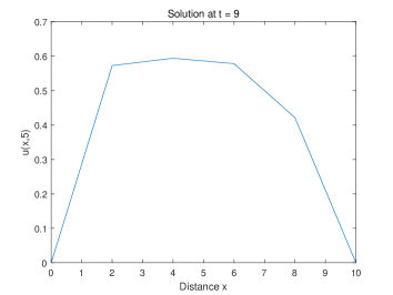
The idea of discrete partitions is illustrated in this example, and points are chosen to describe the temperature along the rod. A point whose value is greater than 0.7 will be moved to mode OFF and be moved back to ON as the value drops below 0.4. The initial temperature is everywhere on the rod, and the input function for mode ON is and for mode OFF. Since we have the boundary condition and , the two values, and , will decrease rapidly due to the heat diffusion effect [20]. Additionally, the input function decreases as increases, therefore the heating effect near the boundary will be trivial, and the heater remains on. We discretize the domain and assign each mesh point a heater. The center difference scheme is used to approximate the space derivative and the forward scheme is used to approximate the time derivative.
Mathematically speaking, we can see even though the discretization reduces the model in HA for ODE, in the following analysis we can see the dynamic of the solutions is consistent with the diffusion feature of the PDE model: consider the following ODE system
| (10) |
where and . Initially, we have , (10) is an ODE system with constant coefficients, hence the existence, uniqueness and continuous dependence follows from the standard ODE theory. Furthermore, it is easy to see that
in other words, is increasing initially since the heat source is turned ON. If there are some hits the threshold value , we may pick the maximum value, say , then since the heat source is turned OFF, we have
where we use the fact that , and . This implies that starts to decrease. For locations that are away from the boundary, if the value falls into , we pick the minimum value, then we have that
where we use the fact that and Therefore, starts to increase again. We conclude that invariant region for , is . For and , we claim that their values cannot fall below , in fact, from the OFF mode, when and go down to 0, we have
which means the values of and will start to go up again which prevents the values fall further into negatives. Hence, the invariant region for and is .
Traffic Flow Model.
We consider the model appearing in [26]. The switched PDE problem is a LWR PDE [24] with the triangular flux function. The flux function and two PDE modes are:
| (11) |
We chose , , and . The forward traffic flow maintains a speed equal to and the backward wave maintains a speed equal to . Moreover, equals which is the guard condition for switching. Lastly, is the parameter specified in backward wave. The diagram of the model is in Figure 11.
Initially, the regions, , are assigned a value for free flow mode. The other remaining areas, , are assigned a value for congestion mode. The Equation 11 shows the free flow mode carries the traffic forward and congestion pushes the traffic backwards. Once the forward and backward waves meet each other, the forward wave merges into the backward wave and starts to move back. The traffic leaves the system and no longer enters again when it reaches the boundary. For simplicity, no incoming traffic is considered.
We can facilitate simulation if we harness the theoretical aspects of linear hyperbolic equations. To simulate the first-order wave equation, only a one-side scheme is feasible and the low accuracy of the scheme requires a very dense discretization [46] which makes the computation task a nightmare. Thus, the simulation is just done by moving the waves along the axis. The results are shown in Figure 12(a) and 12(b).
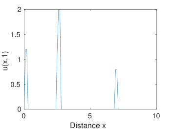
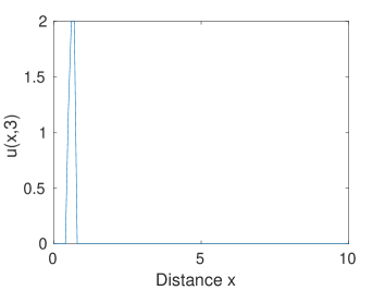
At , the backward wave appearing at the boundary is about to leave. Wave originating from moves to the place around . The forward wave starting at propagates to the region . The discrete partition changes to for points and for points . At , only one single backward wave remains. for and for . Here we use the explicit solutions instead of numerical solutions for the ODE system due to the transport feature of the traffic model. Simulations show that the traffic merges around and eventually all flows leave the system. Around the merging location, the area that used to be in the free mode switches to the congestion mode.
6 Conclusion
In this paper, we propose a theoretical model called PDHA for modelling PDE dynamic systems. PDHA involves novel features such as the notion of domain , which is used to define the spatial location, and domain partition , which is used to describe the mode occupation and domain changing with respect to time. After building the theory for PDHA, we present another model called discrete space PDHA that we construct for the purpose of analysis. In discrete space PDHA, the discretization relation and scheme are proposed to formalize the discrete model. Additionally, the partition and space mode are replaced by a discrete partition, making the analysis easier. Moreover, we formally defined concepts such as time trajectory, model execution, Zeno behavior, reachability analysis, and determinism for DSPDHA. The paper also displays explorations towards the relations of the three models.
Although a few results and similarities are presented regarding DSPDHA and HA, other topics such as invariants, uniqueness, and continuity remain unexplored. The dynamic properties we proposed are only for DSPDHA, there is no similar conclusion for the continuous PDHA. Also, in our examples, we simply consider a one-dimension uniform discretization using easy FDMs. Other approaches like generalized finite difference and finite element methods can also play a critical role if an irregular domain is considered. Deciding DSPDHA from PDHA is also a challenging endeavor. Thus, an approach for measuring the distance between the approximated DSPDHA and real PDHA is deeply needed.
It is worth mentioning that the number of ODEs in the finite difference scheme (FDM) framework depends on the chosen partition. To obtain accurate and highly-resolved solutions, a fine partition becomes indispensable, which consequently leads to high-dimensional ODE systems. In such cases, the use of deep neural network models [48] could potentially offer valuable insights and broaden the applications of our approach. Exploring the potential of deep neural networks in this context is an avenue we plan to investigate in future research.
7 Acknowledgements
W. Xiang was supported by the National Science Foundation, under NSF CAREER Award no. 2143351, and NSF CNS Award no. 2223035.
References
- [1] E. A. Lee, Cyber physical systems: Design challenges, in: 2008 11th IEEE International Symposium on Object and Component-Oriented Real-Time Distributed Computing (ISORC), IEEE, 2008, pp. 363–369.
- [2] S. N. Krishna, A. Trivedi, Hybrid automata for formal modeling and verification of cyber-physical systems, arXiv preprint arXiv:1503.04928.
- [3] H.-D. Tran, W. Xiang, T. T. Johnson, S. Bak, Reachability analysis for one dimensional linear parabolic equations, 6th IFAC Conference on Analysis and Design of Hybrid Systems.
- [4] W. Xiang, On equivalence of two stability criteria for continuous-time switched systems with dwell time constraint, Automatica 54 (2015) 36–40.
- [5] W. Xiang, Necessary and sufficient condition for stability of switched uncertain linear systems under dwell-time constraint, IEEE Transactions on Automatic Control 61 (11) (2016) 3619–3624.
- [6] W. Xiang, Parameter-memorized lyapunov functions for discrete-time systems with time-varying parametric uncertainties, Automatica 87 (2018) 450–454.
- [7] W. Xiang, J. Lam, J. Shen, Stability analysis and l1-gain characterization for switched positive systems under dwell-time constraint, Automatica 85 (2017) 1–8.
- [8] W. Xiang, H.-D. Tran, T. T. Johnson, Robust exponential stability and disturbance attenuation for discrete-time switched systems under arbitrary switching, IEEE Transactions on Automatic Control 63 (5) (2017) 1450–1456.
- [9] L. Zhang, W. Xiang, Mode-identifying time estimation and switching-delay tolerant control for switched systems: An elementary time unit approach, Automatica 64 (2016) 174–181.
- [10] Z. Xu, H. Su, P. Shi, R. Lu, Z.-G. Wu, Reachable set estimation for markovian jump neural networks with time-varying delays, IEEE transactions on cybernetics 47 (10) (2016) 3208–3217.
- [11] W. Xiang, H.-D. Tran, T. T. Johnson, Output reachable set estimation for switched linear systems and its application in safety verification, IEEE Transactions on Automatic Control 62 (10) (2017) 5380–5387.
- [12] W. Xiang, H.-D. Tran, T. T. Johnson, On reachable set estimation for discrete-time switched linear systems under arbitrary switching, in: 2017 American Control Conference (ACC), IEEE, 2017, pp. 4534–4539.
- [13] M. Johansson, A. Rantzer, Computation of piecewise quadratic lyapunov functions for hybrid systems, in: 1997 European Control Conference (ECC), IEEE, 1997, pp. 2005–2010.
- [14] M. Margaliot, G. Langholz, Necessary and sufficient conditions for absolute stability: the case of second-order systems, IEEE Transactions on Circuits and Systems I: Fundamental Theory and Applications 50 (2) (2003) 227–234.
- [15] S. Pettersson, B. Lennartson, Stabilization of hybrid systems using a min-projection strategy, in: Proceedings of the 2001 American Control Conference.(Cat. No. 01CH37148), Vol. 1, IEEE, 2001, pp. 223–228.
- [16] A. S. Morse, Supervisory control of families of linear set-point controllers-part i. exact matching, IEEE transactions on Automatic Control 41 (10) (1996) 1413–1431.
- [17] L. I. Allerhand, U. Shaked, Robust stability and stabilization of linear switched systems with dwell time, IEEE Transactions on Automatic Control 56 (2) (2010) 381–386.
- [18] J. P. Hespanha, A. S. Morse, Stability of switched systems with average dwell-time, in: Proceedings of the 38th IEEE conference on decision and control (Cat. No. 99CH36304), Vol. 3, IEEE, 1999, pp. 2655–2660.
- [19] L. Zhang, H. Gao, Asynchronously switched control of switched linear systems with average dwell time, Automatica 46 (5) (2010) 953–958.
- [20] L. C. Evans, Partial differential equations, American Mathematical Society.
- [21] T. Bao, X. Jia, J. Zwart, J. Sadler, A. Appling, S. Oliver, T. T. Johnson, Partial differential equation driven dynamic graph networks for predicting stream water temperature, in: 2021 IEEE International Conference on Data Mining (ICDM), IEEE, 2021, pp. 11–20.
- [22] T. Bao, S. Chen, T. T. Johnson, P. Givi, S. Sammak, X. Jia, Physics guided neural networks for spatio-temporal super-resolution of turbulent flows, in: Uncertainty in Artificial Intelligence, PMLR, 2022, pp. 118–128.
- [23] A. M. Bayen, R. L. Raffard, C. J. Tomlin, Network congestion alleviation using adjoint hybrid control: Application to highways, in: International Workshop on Hybrid Systems: Computation and Control, Springer, 2004, pp. 95–110.
- [24] M. J. Lighthill, G. B. Whitham, On kinematic waves ii. a theory of traffic flow on long crowded roads, Proc. R. Soc. Lond. A 229 (1178) (1955) 317–345.
- [25] L. Muñoz, X. Sun, R. Horowitz, L. Alvarez, Traffic density estimation with the cell transmission model, in: American Control Conference, 2003. Proceedings of the 2003, Vol. 5, IEEE, 2003, pp. 3750–3755.
- [26] C. G. Claudel, A. M. Bayen, Solutions to switched Hamilton–Jacobi equations and conservation laws using hybrid components, in: International Workshop on Hybrid Systems: Computation and Control, Springer, 2008, pp. 101–115.
- [27] T. A. Henzinger, The theory of hybrid automata, in: Proceedings 11th Annual IEEE Symposium on Logic in Computer Science, IEEE, 1996, pp. 278–292.
- [28] R. Alur, C. Courcoubetis, T. A. Henzinger, P.-H. Ho, Hybrid automata: An algorithmic approach to the specification and verification of hybrid systems, in: International Hybrid Systems Workshop, Springer, 1991, pp. 209–229.
- [29] T. Bao, et al., Modelling physics-based dynamic system using machine learning, Ph.D. thesis, Vanderbilt University (2023).
- [30] D. G. Mallet, L. G. De Pillis, A cellular automata model of tumor–immune system interactions, Journal of theoretical biology 239 (3) (2006) 334–350.
- [31] A. Banerjee, S. K. Gupta, Spatio-temporal hybrid automata for safe cyber-physical systems: A medical case study, in: Proceedings of the ACM/IEEE 4th International Conference on Cyber-Physical Systems, 2013, pp. 71–80.
- [32] C. Tomlin, J. Lygeros, S. Sastry, Computing controllers for nonlinear hybrid systems, in: Hybrid Systems: Computation and Control: Second International Workshop, HSCC’99 Berg en Dal, The Netherlands, March 29–31, 1999 Proceedings 2, Springer, 1999, pp. 238–255.
- [33] R. Bonnerot, P. Jamet, Numerical computation of the free boundary for the two-dimensional stefan problem by space-time finite elements, Journal of Computational Physics 25 (2) (1977) 163–181.
- [34] J. M. Aitchison, S. Howison, Computation of hele-shaw flows with free boundaries, Journal of Computational Physics 60 (3) (1985) 376–390.
- [35] A. Friedman, V. Principles, Free boundary problems, Malabar, Fla.: RE Krieger 258.
- [36] L. A. Caffarelli, S. Salsa, S. Salsa, A geometric approach to free boundary problems, Vol. 68, American Mathematical Soc., 2005.
- [37] A. Friedman, Free boundary problems in science and technology, Notices of the AMS 47 (8) (2000) 854–861.
- [38] G. Ryskin, L. Leal, Numerical solution of free-boundary problems in fluid mechanics. part 1. the finite-difference technique, Journal of fluid mechanics 148 (1984) 1–17.
- [39] G. Ryskin, L. Leal, Numerical solution of free-boundary problems in fluid mechanics. part 2. buoyancy-driven motion of a gas bubble through a quiescent liquid, Journal of Fluid Mechanics 148 (1984) 19–35.
- [40] F. M. Hante, G. Leugering, T. I. Seidman, Modeling and analysis of modal switching in networked transport systems, Applied Mathematics and Optimization 59 (2) (2009) 275–292.
- [41] C. J. Tomlin, J. Lygeros, S. S. Sastry, A game theoretic approach to controller design for hybrid systems, Proceedings of the IEEE 88 (7) (2000) 949–970.
- [42] I. S. Strub, A. M. Bayen, Weak formulation of boundary conditions for scalar conservation laws: An application to highway traffic modelling, International Journal of Robust and Nonlinear Control: IFAC-Affiliated Journal 16 (16) (2006) 733–748.
- [43] P. R. Halmos, Naive set theory, Courier Dover Publications, 2017.
- [44] G. D. Smith, Numerical solution of partial differential equations: finite difference methods, Oxford university press, 1985.
- [45] J. Lygeros, K. H. Johansson, S. N. Simic, J. Zhang, S. S. Sastry, Dynamical properties of hybrid automata, IEEE Transactions on automatic control 48 (1) (2003) 2–17.
- [46] J. W. Thomas, Numerical partial differential equations: finite difference methods, Vol. 22, Springer Science & Business Media, 2013.
- [47] J. Rauch, M. Reed, Jump discontinuities of semilinear, strictly hyperbolic systems in two variables: Creation and propagation, Communications in Mathematical Physics 81 (2) (1981) 203–227.
- [48] R. T. Chen, Y. Rubanova, J. Bettencourt, D. K. Duvenaud, Neural ordinary differential equations, Advances in neural information processing systems 31.