A New Many-Objective Evolutionary Algorithm Based on Determinantal Point Processes

Peng Zhang, Jinlong Li, Tengfei Li, and Huanhuan Chen P. Zhang, J. Li, T. Li and H. Chen are with School of Computer Science and Technology, University of Science and Technology of China, Hefei 230027, China (e-mail: zp1996@mail.ustc.edu.cn; jlli@ustc.edu.cn; ltf91@mail.ustc.edu.cn; hchen@ustc.edu.cn). Corresponding author: Jinlong LiThis research work was supported by the National Natural Science Foundation of China under Grants 61573328

Abstract

To handle different types of Many-Objective Optimization Problems (MaOPs), Many-Objective Evolutionary Algorithms (MaOEAs) need to simultaneously maintain convergence and population diversity in the high-dimensional objective space. In order to balance the relationship between diversity and convergence, we introduce a Kernel Matrix and probability model called Determinantal Point Processes (DPPs). Our Many-Objective Evolutionary Algorithm with Determinantal Point Processes (MaOEADPPs) is presented and compared with several state-of-the-art algorithms on various types of MaOPs with different numbers of objectives. The experimental results demonstrate that MaOEADPPs is competitive.

Index Terms:

Convergence, diversity, evolutionary algorithm, many-objective optimization, Determinantal Point Processes.

I INTRODUCTION

Many practical problems can be treated as Many-objective Optimization Problems (MaOPs), such as ensemble learning [1, 2], engineering design [3], time series learning [4]. An MaOP can be expressed by Equation (1):

\begin{split}{\rm M}&{\rm inimize}\quad\boldsymbol{F(x)}=(f_{1}(\boldsymbol{x}),f_{2}(\boldsymbol{x}),\dots,f_{M}(\boldsymbol{x}))^{T}\\ {\rm su}&{\rm bject\>to}\quad\boldsymbol{x}\in\boldsymbol{\Omega},\end{split}

(1)

where $\boldsymbol{x}=(x_{1},x_{2},\dots,x_{n})^{T}$ is an $n$ -dimensional decision vector in the decision space $\boldsymbol{\Omega}$ , $M>3$ is the number of objectives, and $\boldsymbol{F}(x)$ is the $M$ -dimensional objective vector.

When solving MaOPs with Many-Objective Evolutionary Algorithms (MaOEAs), the incomparability of solutions causes the proportion of nondominated solutions to increase enormously [5, 6]. This makes optimization using only the domination relationship infeasible. It is also difficult to maintain population diversity in a high-dimensional objective space [5]. In order to solve these two problems, researchers have proposed several methods, most of which can be roughly divided into three categories.

The Pareto dominance-based MaOEAs belong to the first category, which employs modified Pareto dominance-based mechanisms to select nondominated solutions. For instance, $\epsilon$ -dominance [7] and fuzzy dominance [8] employ modified definitions of dominance to maintain the selection pressure. Different distance measures are used to improve the performance of Pareto dominance-based MaOEAs [9, 10]. Zhang et al. employ a knee point-based selection scheme to select nondominated solutions [11]. Li et al. propose a shift-based density estimation strategy to make Pareto dominance-based algorithms more suitable for many-objective optimization [12].

Indicator-based MaOEAs form the second category. These MaOEAs use indicators to evaluate the solutions and guide the search process. The hypervolume (HV) [13, 14] is one widely used indicator. The HypE employs Monte Carlo simulation to estimate the HV contribution of the candidate solutions and reduce the high complexity of calculating the HV [15]. Other popular indicators include the R2 indicator [16] and the Inverted Generational Distance (IGD) [17]. For instance, MOMBI selects offspring based on the R2 indicator [18], and MyO-DEMR combines the concept of Pareto dominance with the IGD to select the next generation [19]. Moreover, the Indicator-based Evolutionary Algorithm (IBEA) can be integrated with arbitrary indicators [20].

The algorithms in the third category, decomposition-based MaOEAs, decompose an MaOP into a number of single-objective optimization problems (SOPs) or simpler MOPs to be solved collaboratively. On the one hand, some decomposition-based MOEAs such as reference vector guided EA (RVEA) [21] and MOEA based on decomposition (MOEA/D) [22] decompose an MOP into a number of SOPs. On the other hand, some other decomposition-based MOEAs such as NSGA-III [23] and SPEA based on reference direction [24] decompose an MOP into several simpler MOPs by dividing the objective space into several subspaces.

Despite many research efforts, the studies on MaOPs are still far from satisfactory. Most of the current studies focus on MaOPs with fewer than 15 objectives [25, 26]. To address this problem, we propose a new Many-Objective Evolutionary Algorithm with Determinantal Point Processes (MaOEADPPs), which performs very well on a variety of types of test instances with the number of objectives ranging from 5 to 30. Our MaOEADPPs quantitatively calculates the distribution of all solutions in the population using a Kernel Matrix. The Kernel Matrix can be split into quality and similarity components, which represent the diversity and convergence of the population, respectively. Determinantal Point Processes (DPPs) are then employed to select the solutions with higher diversity and convergence based on the decomposition of the Kernel Matrix. To further improve the performance of the Kernel Matrix, we introduce corner solutions [27].

The main contributions of this paper are summarized as follows.

1.

In order to adapt to different types of MaOPs and different objectives, we propose a new Kernel Matrix in which a similarity measure is defined as the cosine value of the angle between two solutions and the quality of a solution is measured by the $L_{2}$ norm of its objective vector.
2.

We propose Determinantal Point Processes Selection (DPPs-Selection) to select a subset of the population. We then integrate the DPPs-Selection and the Kernel Matrix to obtain the new Many-Objective Evolutionary Algorithm with Determinantal Point Processes (MaOEADPPs).

The rest of this paper is organized as follows. In Section II, we introduce the background knowledge. In Section III, we describe the details of our new algorithm. After that, the experimental results are given in Section IV. Finally, we summarize this paper and discuss the future work in Section V.

II BACKGROUND

II-A Determinantal Point Processes

Determinantal Point Processes (DPPs) have been used in subset selection tasks such as product recommendation [28], text summarization [29], web search [30], and graph sampling [31]. As shown in Equation (2), a point process is a probabilistic measure for one instantiation $Y$ of a set $\mathbf{Y}$ . We assume discrete finite point processes, i.e., $\mathbf{Y}=\{1..N\}$ .

\mathcal{P}_{\mathbf{L}}(Y=\mathbf{Y})=\frac{\operatorname{det}\left(\mathbf{L}_{Y}\right)}{\operatorname{det}(\mathbf{L}+\mathbf{I})}

(2)

where $\mathbf{L}$ is an $N\times N$ semi-definite Kernel Matrix indexed by $\{1..N\}$ , $\mathbf{I}$ is the $N\times N$ identity matrix, and $\rm det(\cdot)$ is the determinant. $\mathbf{L}_{Y}$ is the Kernel Matrix $\mathbf{L}$ with indices restricted by entries indexed in the subset $Y$ . For example, if the subset is restricted to one element $Y=\{i\}$ , then $\mathbf{L}_{Y}={L}_{ii}$ . The element $L_{ij}$ measures the similarity of $i$ ^th and $j$ ^th elements in the set $\mathbf{Y}$ . If we restrict the cardinality of the instantiation $Y$ to $k$ , the Determinantal Point Processes are called $k$ -DPPs. In this case, Equation (3) holds:

\mathcal{P}_{\mathbf{L}}^{k}(Y=\mathbf{Y})=\frac{\operatorname{det}\left(\mathbf{L}_{Y}\right)}{\sum_{\left|Y^{\prime}\right|=k}\operatorname{det}\left(\mathbf{L}_{Y^{\prime}}\right)}

(3)

To reduce the cost of calculating $\mathcal{P}_{\mathbf{L}}^{k}(Y)$ , which requires $O\left(N^{k}\right)$ steps, Kulesza and Taskar proposed the following method [30]. First, the Kernel Matrix $\mathbf{L}$ is eigen-decomposed $\mathbf{L}=\sum_{n=1}^{N}\lambda_{n}\mathbf{v}_{n}\mathbf{v}_{n}^{T}$ with a set of eigenvectors $\mathbf{V}$ and eigenvalues $\lambda$ . If $\mathbf{J}$ constitutes a set of $k$ selected eigenvectors and $J$ is an instantiation of $\mathbf{J}$ , the probability for $J$ can be derived as

\operatorname{Pr}(J=\mathbf{J})=\frac{\prod_{n\in J}\lambda_{n}}{\sum_{|J|=k}\prod_{m\in J}\lambda_{m}}

(4)

In the denominator, the sum goes over all possible instantiations $J$ of $\mathbf{J}$ . Here $Pr$ denotes the probability, whereas $\mathcal{P}_{\mathrm{L}}(Y=\mathbf{Y})$ is a probability measure. In [29], it is shown that when sampling from DPPs, the probability of an element $i$ from $\mathbf{Y}$ , is given by

Pr(i)=\frac{1}{\mathbf{V}}\sum_{\mathbf{v}\in\mathbf{V}}\left(\mathbf{v}^{T}e_{i}\right)^{2}

(5)

where $e_{i}$ is the $i$ ^th unit vector $e_{i}=(0,\dots,1,\dots,0)$ , with all elements 0 except the element at index $i$ , which is 1.

II-B Corner Solution

In the MaOPs, a majority of solutions in the population will become nondominated after several generations [5]. This often causes the algorithms to lose the selection pressure. To solve this problem, we modify the definition of solution quality with the assistance of corner solutions [27]. If we get just one solution when minimizing $k$ of $M$ objectives, this solution is called a corner solution. However, Ran and Ishibuchi point out that the corner solutions for $k>1$ are difficult to find [32, 33]. Therefore, we will propose approximation methods to search for corner solutions in Section III.

III PROPOSED ALGORITHM: MaOEADPPs

First, the general framework of MaOEADPPs is reported. Then, we will describe the calculation of the Kernel Matrix. After that, the details of Environmental Selection and other important components of MaOEADPPs are explained one by one.

III-A General Framework of MaOEADPPs

The pseudocode of MaOEADPPs is given in Algorithm 1. First, an initial population $\boldsymbol{P}$ is filled with $N$ random solutions. Then, a Corner Solution Archive $\boldsymbol{CSA}$ is extracted from $\boldsymbol{P}$ . Based on $\boldsymbol{P}$ , the ideal point $z^{*}$ and the nadir point $z^{nad}$ are initialized in steps 3-4, where $z_{i}^{*}$ and $z_{i}^{nad}$ are calculated by Equations (6) and (7):

	$\displaystyle z^{*}$	$\displaystyle=\left(z_{1}^{},z_{2}^{},\ldots,z_{m}^{*}\right)^{T}$		(6)
	$\displaystyle z_{i}^{*}$	$\displaystyle=\min(\left\{\left(f_{i}(x)\right)\|x\in\boldsymbol{P}\right\})$		(6)

	$\displaystyle z^{nad}$	$\displaystyle=\left(z_{1}^{nad},z_{2}^{nad},\ldots,z_{m}^{nad}\right)^{T}$		(7)
	$\displaystyle z_{i}^{nad}$	$\displaystyle=\max(\left\{\left(f_{i}(x)\right)\|x\in\boldsymbol{P}\right\})$		(7)

${z}_{i}^{*}$ and $z_{i}^{nad}$ are used to normalize the objective values $f_{i}(x)$ , as shown by Equation (8). This is important because the objective functions could have vastly different scales.

f_{i}(x)=\dfrac{f_{i}(x)-{z}_{i}^{*}}{z_{i}^{nad}-{z}_{i}^{*}}.

(8)

Next, steps 5-12 are iterated until the number of function evaluations exceeds a fixed limit (100’000 in our experiments). At each iteration, $2N$ solutions are selected as the mating pool $\boldsymbol{P}^{\prime}$ . Simulated binary crossover (SBX) [34] and polynomial mutation [35] are employed to generate the candidate population $\boldsymbol{C}$ . Then the ideal point $\boldsymbol{z}^{*}$ is updated by Equation (6). After Environmental Selection, $z^{nad}$ will be updated by Equation (7).

Algorithm 1 Framework of the proposed MaOEADPPs

N

(population size)

\boldsymbol{P}\leftarrow\

Initialize Population(

N

)

\boldsymbol{CSA}

\leftarrow\

\boldsymbol{P}

\boldsymbol{z}^{*}\leftarrow\

Initialize Ideal Point(

\boldsymbol{P}

)

\boldsymbol{z}^{nad}\leftarrow\

Initialize Nadir Point(

\boldsymbol{P}

)

5: while the number of function evaluations does not exceed 100’000 do

\boldsymbol{P}^{\prime}\leftarrow

Filling the Mating Pool(

\boldsymbol{P},\boldsymbol{CSA},N,\boldsymbol{z}^{*},\boldsymbol{z}^{nad}

)

\boldsymbol{C}\leftarrow

Variation(

\boldsymbol{P}^{\prime}

)

\boldsymbol{z}^{*}\leftarrow\

Update Ideal Point(

\boldsymbol{z}^{*},\boldsymbol{C}

)

\boldsymbol{CSA}

\leftarrow

UpdateCSA(

\boldsymbol{CSA},\boldsymbol{C},N

)

10:

\boldsymbol{P}

\leftarrow

Environmental Selection(

\boldsymbol{P},\boldsymbol{C},N,\boldsymbol{CSA},\boldsymbol{z}^{*},\boldsymbol{z}^{nad}

)

11:

\boldsymbol{z}^{nad}\leftarrow\

Update Nadir Point(

\boldsymbol{P},\boldsymbol{CSA}

)

12: end while

12:

\boldsymbol{P}

III-B Filling the Mating Pool

To produce high-quality offspring, we generate the mating pool $\boldsymbol{P}^{\prime}$ by selecting elements from the union of $\boldsymbol{P}$ and $\boldsymbol{CSA}$ . We therefore define the convergence $con(x)$ of a solution $x\in\boldsymbol{P}$ according to Equation (9):

con(x)={\frac{1}{\sum_{i=1}^{m}(f_{i}(x))^{2}}}

(9)

Then, as illustrated in Algorithm 2, we randomly choose a solution $x$ from the union $\boldsymbol{P}\cup\boldsymbol{CSA}$ . If the convergence $con(y)$ of solution $y=\underset{y\in\boldsymbol{P}}{\arg\min}\{\cos(x,y)\}$ is greater than $con(x)$ and a randomly generated number is less than a threshold $\delta(x,y)$ , $y$ is added to $\boldsymbol{P}^{\prime}$ . Otherwise, $x$ is added to $\boldsymbol{P}^{\prime}$ . The threshold $\delta(x,y)$ is computed according to Equation (10).

\begin{split}&\delta(x,y)=\frac{\cos(x,y)-minCos}{maxCos-minCos}\\ &maxCos=\max\limits_{p,q\in\boldsymbol{P}\cup\boldsymbol{CSA},p\neq q}\{\cos(p,q)\}\\ &minCos=\min\limits_{p,q\in\boldsymbol{P}\cup\boldsymbol{CSA},p\neq q}\{\cos(p,q)\}\end{split}

(10)

Each time offspring needs to be generated, two solutions are randomly selected from mating pool $\boldsymbol{P}^{\prime}$ as the parents.

Algorithm 2 Filling the Mating Pool

\boldsymbol{P}

(population),

\boldsymbol{CSA}

(Corner Solution Archive),

N

(population size),

z^{*}

(ideal point),

z^{nad}

(nadir point)

1: Normalization(

\boldsymbol{P}\cup\boldsymbol{CSA}

z^{*}

z^{nad}

)

\boldsymbol{P}^{\prime}\leftarrow\emptyset

3: for

i=1\to 2N

4: Randomly select

x

from

\boldsymbol{P}\cup\boldsymbol{CSA}

5: Find solution

y=\underset{y\in\boldsymbol{P}}{\arg\min}\{\cos(x,y)\}

6: if

(rand<\delta\wedge({con}(y)>{con}(x))

then

\boldsymbol{P}^{\prime}

\leftarrow

\boldsymbol{P}^{\prime}\bigcup\{y\}

8: else

\boldsymbol{P}^{\prime}

\leftarrow

\boldsymbol{P}^{\prime}\bigcup\{x\}

10: end if

11: end for

11:

\boldsymbol{P}^{\prime}

III-C Environmental Selection

Algorithm 3 Environmental Selection

\boldsymbol{P}

(population),

\boldsymbol{C}

(candidate population),

N

(population size),

\boldsymbol{CSA}

(Corner Solution Archive),

z^{*}

(ideal point),

z^{nad}

(nadir point)

P\leftarrow\

Nondominated(

\boldsymbol{P}\cup\boldsymbol{C}

)

2: if

|\boldsymbol{P}|>N

then

3: Normalization(

\boldsymbol{CSA}

z^{*}

z^{nad}

)

4: Normalization(

\boldsymbol{P}

\boldsymbol{z}^{*}

z^{nad}

)

\boldsymbol{L}

\leftarrow

Calculation of the Kernel Matrix(

\boldsymbol{P}

\boldsymbol{CSA}

)

\boldsymbol{A}

\leftarrow

DPPs-Selection(

\boldsymbol{L}

N

)

\boldsymbol{P}\leftarrow\boldsymbol{P}(\boldsymbol{A})

8: end if

\boldsymbol{P}

The framework of Environmental Selection is given in Algorithm 3. First, the nondominated solutions are selected from the union of $\boldsymbol{P}$ and $\boldsymbol{C}$ . If the number of nondominated solutions is greater than $N$ , we calculate the Kernel Matrix $\boldsymbol{L}$ and update $\boldsymbol{P}$ with DPPs-Selection.

The Kernel Matrix $\boldsymbol{L}$ is defined to represent both the diversity and the convergence of the population. We use Equation (11) to calculate its elements ${L}_{xy}$ :

{L}_{xy}=q(x)S(x,y)q(y)

(11)

where $x,y\in\boldsymbol{P}$ , $q(x)$ is the quality of solution $x$ , and $S(x,y)$ is the similarity between elements $x$ and $y$ . To measure the similarity between $x$ and $y$ , $S(x,y)$ is defined by Equation (12).

S(x,y)=\exp{(-\cos(x,y))}

(12)

where $\cos(x,y)$ is the cosine of the angle between solutions $x$ and $y$ . The quality $q(x)$ of solution $x$ is calculated based on its convergence, as shown by Equations (13) and (14).

q(x)=\begin{cases}{con}_{1}(x)&x\in outside\>space\\ 2*\max\limits_{p\in\boldsymbol{P}}({con}_{1}(p))&x\in inside\>space\end{cases}

(13)

{con}_{1}(x)=\dfrac{con(x)}{\max\limits_{p\in\boldsymbol{P}}(con(p))}

(14)

where ${con}_{1}$ is the normalized convergence. $outside\ space$ and $inside\ space$ describe the different areas of the objective space. If $\sqrt{\sum_{i=1}^{M}f_{i}(x)^{2}}\leq\operatorname{t}$ , the solution $x$ belongs to the $inside\ space$ and otherwise to the $outside\ space$ . The threshold $t$ is set to $t=\max{\left\{\left.\sqrt{\sum_{i=1}^{M}f_{i}(x)^{2}}\right|x\in\boldsymbol{CSA}\right\}}$ .

The Corner Solution Archive $\boldsymbol{CSA}$ is used to distinguish the $outside\ space$ and $inside\ space$ . Since it is difficult to find the corner solutions for $k>1$ [32, 33], we use an approximation method to generate the $\boldsymbol{CSA}$ . According to the value of $k$ , we discuss the corner solutions in two cases.

$\boldsymbol{k=1}$ : To find the corner solutions of objective

$i=1,2,...,M$ , we sort the solutions in ascending order of the objective value $f_{i}$ , so we have $M$ sorted lists and we add the first $\lceil\frac{N}{3M}\rceil$ solutions of each list into the $\boldsymbol{CSA}$ .

$\boldsymbol{1<k<M}$ : We only consider $k=M-1$ and employ an approximation method to get the $\boldsymbol{CSA}$ . For any objective $i=1,2,...,M$ , we sort the solutions in ascending order of $\sqrt{\sum_{j=1,j\neq i}^{M}(f_{j}(x))^{2}}$ and obtain $M$ sorted lists. The first $\lceil\frac{2N}{3M}\rceil$ solutions of each list are selected into the $\boldsymbol{CSA}$ .

From the above two cases, we get $|\boldsymbol{CSA}|=\lceil\frac{N}{3M}\rceil\times M+\lceil\frac{2N}{3M}\rceil\times M\approx N$ . That is each objective contributes $\lceil\frac{N}{M}\rceil$ solutions to the $\boldsymbol{CSA}$ .

Algorithm 4 shows the details of calculating the Kernel Matrix. After calculating the cosine of the angle between every two solutions in the population, the quality $q(x)$ of each solution $x$ is computed. The row vector $\boldsymbol{q}$ then contains the qualities of all solutions. After that, a quality matrix $\boldsymbol{Q}$ is generated as the product of $\boldsymbol{q}^{T}$ and $\boldsymbol{q}$ . Finally, $\boldsymbol{Q}$ is multiplied with $\boldsymbol{L}$ in element-wised manner to update and output $\boldsymbol{L}$ . In step 10, ‘ $\otimes$ ’ indicates the element-wised multiplication of two matrices with the same size.

Algorithm 4 Calculation of the Kernel Matrix

\boldsymbol{P}

(population),

\boldsymbol{CSA}

(Corner Solution Archive)

1: for solution

x\in\boldsymbol{P}

2: for solution

y\in\boldsymbol{P}

\boldsymbol{L}_{xy}=cos(x,y)

4: end for

5: end for

6: for solution

x\in\boldsymbol{P}

7: calculate

q(x)

by Equations (13) and (14)

8: end for

\boldsymbol{Q}=\boldsymbol{q}^{T}\cdot\boldsymbol{q}

10:

\boldsymbol{L}=\boldsymbol{L}\otimes\boldsymbol{Q}

10:

\boldsymbol{L}

In Algorithm 5, we specify the details of the Determinantal Point Processes Selection (DPPs-Selection). First, the $N\times N$ Kernel Matrix $\boldsymbol{L}$ is eigen-decomposed to obtain the eigenvector set $\boldsymbol{V}=\{\boldsymbol{v}_{r}\}^{N}_{r=1}$ and the eigenvalue set $\boldsymbol{\lambda}=\{\lambda_{r}\}^{N}_{r=1}$ . Then, $\{\boldsymbol{v}_{r}\}^{N}_{r=1}$ is sorted in decreasing order of the eigenvalues and is truncated by keeping the $k$ largest eigenvectors only. After that, on each iteration of the while-loop, the index of the element that has the maximum $\sum_{\boldsymbol{v}\in\boldsymbol{V}}(\boldsymbol{v}^{\top}\boldsymbol{e}_{i})^{2}$ is added into the index set $\boldsymbol{S}$ , where the dimension of $\boldsymbol{e}_{i}$ is $N$ and $\boldsymbol{e}_{i}=(0,0,\dots,1,\dots,0,0)$ is the $i$ ^th standard unit vector in $\mathbb{R}^{N}$ . Then $\boldsymbol{V}$ is replaced by an orthonormal basis for the subspace of $\boldsymbol{V}$ orthogonal to $\boldsymbol{e}_{i}$ . Finally, the index set $\boldsymbol{S}$ of the selected elements is returned. In summary, DPPs-Selection has two phases: It first selects $k$ eigenvectors of $\boldsymbol{L}$ that have the maximum corresponding $\lambda$ . Then, it selects the indices of elements that have the maximum $\sum_{\boldsymbol{v}\in\boldsymbol{V}}(\boldsymbol{v^{\top}}\boldsymbol{e}_{i})^{2}$ one by one.

Algorithm 5 DPPs-Selection

\boldsymbol{L}

(Kernel Matrix),

k

(size of subset)

(\{\boldsymbol{v}_{r}\}^{N}_{r=1},\{\lambda_{r}\}^{N}_{r=1})\leftarrow

Eigen-decomposition(

\boldsymbol{L}

)

\boldsymbol{V}\leftarrow

Select

k

eigenvectors from

\{\boldsymbol{v}_{r}\}^{N}_{r=1}

according to the largest

k

eigenvalues in

\{\lambda_{r}\}^{N}_{r=1}

\boldsymbol{S}\leftarrow\phi

4: while

|\boldsymbol{V}|>0

5: Select

i

from

N

that has maximum

\sum_{\boldsymbol{v}\in\boldsymbol{V}}(\boldsymbol{v^{\top}e}_{i})^{2}

\boldsymbol{S}\leftarrow\boldsymbol{S}\cup i

\boldsymbol{V}\leftarrow\boldsymbol{V}_{\perp}

, an orthonormal basis for the subspace of

\boldsymbol{V}

orthogonal to

\boldsymbol{e}_{i}

8: end while

\boldsymbol{S}

IV EXPERIMENTAL STUDY

To evaluate the performance of MaOEADPPs, we compare it with the state-of-the-art algorithms NSGA-III [36], RSEA [37], $\theta$ -DEA [38], AR-MOEA [39], and RVEA [40] on a set of benchmark problems with 5, 10, 13, 15, 20, 25, and 30 objective functions. After that, we investigate the effectiveness of our new Kernel Matrix and DPPs-Selection. All the experiments are conducted using PlatEMO [41], which is an evolutionary multi-objective optimization platform.

IV-A Test Problems and Performance Indicators

To evaluate our methods under a wide variety of different problems types, we choose the benchmarks DTLZ1-DTLZ6 [42], IDTLZ1 and IDTLZ2 [43], WFG1-WFG9 [44], and MAF1-MAF7 [32].

WFG1 is a separable and unimodal problem. WFG2 has a scaled-disconnected PF and WFG3 has a linear PF. WFG4 introduces multi-modality to test the ability of algorithms to jump out of local optima. WFG5 is a highly deceptive problem. The nonseparable reduction of WFG6 is difficult. WFG7 is a separable and unimodal problem. WFG8 and WFG9 introduce significant bias to evaluate the MaOEA performance.

DTLZ1 is a simple test problem with a triangular PF. DTLZ2 to DTLZ4 have concave PFs. DTLZ5 tests the ability of an MaOEA to converge to a curve. DTLZ6 is a modified version of DTLZ5. IDTLZ1 and IDTLZ2 are obtained by inverting the PFs of DTLZ1 and DTLZ2, respectively.

MaF1 is a modified inverted instance of DTLZ1. MaF2 is modified from DTLZ2 to increase the difficulty of convergence. MaF3 is a convex version of DTLZ3. MaF4 is used to assess a MaOEA performance on problems with badly scaled PFs. MaF5 has a highly biased solution distribution. MaF6 is used to assess whether MaOEAs are capable of dealing with degenerate PFs. MaF7 is used to assess MaOEAs on problems with disconnected PFs.

Following the settings in the original papers [42, 43, 44, 32], for DTLZ2-DTLZ4, MaF1-MaF7, IDTLZ2 and WFG1-WFG9, the numbers of decision variables $D$ are set to $M-1+10$ , where $M$ denotes the number of objectives. For IDTLZ1 and DTLZ1, the numbers of decision variables $D$ are set to $M-1+5$ . As performance metrics, we adopt the widely used IGD [45] and HV [44] indicators.

IV-B Experimental Settings

Population size: The population size in our experiments is the same as the number of reference points. The reference points are generated by Das and Dennis’s approach [46] with two layers. This method is adapted in NSGA-III, $\theta$ -DEA, and RVEA. For fair comparisons, the population size of all algorithms is set according to Table I. According to the above method, there is no appropriate parameter to ensure that the population size for 13 objectives is less than for 15 objectives and greater than for 10 objectives. We thus set the population size of 13 objectives to be the same as 15 objectives.

Genetic operators: we apply simulated binary crossover (SBX) [34] and polynomial mutation [35] to generate the offspring. The crossover probability $p_{c}$ and the mutation probability $p_{m}$ are set to 1.0 and $1/D$ , respectively, where $D$ denotes the number of decision variables. Both distribution indices of crossover and mutation are set to 20.

TABLE I: POPULATION SIZE SETTINGS

Number of objectives	Parameter	Population size
(M)	( $p_{1}$ , $p_{2}$ )	(N)
5	(5,0)	126
10	(3,1)	230
15	(2,2)	240

Termination condition and the number of runs: The tested algorithms will be terminated when the number of function evaluations exceeds 100’000. All algorithms are executed for 30 independent runs on each test instance.

Parameter settings for algorithms: The two parameters $\alpha$ and $f_{r}$ of RVEA are set to 2 and 0.1, respectively, which is the same as in [40].

IV-C Experimental Results and Analysis

We now analyze the results of the aforementioned state-of-the-art algorithms on our benchmark instances. The mean values and the standard deviations of the IGD and HV metrics on DTLZ1-DTLZ6, IDTLZ1-IDTLZ2 and WFG1-WFG9 with 5, 10, 13, and 15 objectives are listed in Tables II and III, respectively. In each table, the best mean value for each instance is highlighted. The symbols ‘+’, ‘-’, and ‘ $\approx$ ’ indicate whether the results are significantly better than, significantly worse than, or not significantly different from those obtained by MaOEADPPs, respectively. We apply the Wilcoxon rank sum test with a significance level of 0.05.

TABLE II: IGD VALUES OBTAINED BY MAOEADPPS, AR-MOEA [39], NSGA-III [36], RSEA [37],

\theta

-DEA [38] AND RVEA [40] ON DTLZ1-DTLZ6, IDTLZ1-IDTLZ2 AND WFG1-WFG9 WITH 5, 10, 13, AND 15 OBJECTIVES. THE BEST RESULTS FOR EACH INSTANCE ARE HIGHLIGHTED IN GRAY.

Problem	$M$	MaOEADPPs	AR-MOEA	NSGA-III	RSEA	$\theta$ -DEA	RVEA
DTLZ1	5	6.3306e-2 (2.01e-3)	6.3325e-2 (8.43e-5) $-$	6.3377e-2 (6.27e-5) $-$	7.6739e-2 (3.13e-3) $-$	6.3356e-2 (7.85e-5) $-$	6.3322e-2 (4.56e-5) $-$
DTLZ1	10	1.1196e-1 (1.05e-3)	1.3914e-1 (3.67e-3) $-$	1.7758e-1 (8.00e-2) $-$	1.3925e-1 (7.37e-3) $-$	1.3572e-1 (2.74e-2) $-$	1.3167e-1 (2.59e-3) $-$
DTLZ1	13	1.3318e-1 (2.66e-3)	1.3186e-1 (3.36e-3) $+$	1.8794e-1 (5.80e-2) $-$	1.8854e-1 (2.71e-2) $-$	1.3913e-1 (3.37e-2) $-$	1.3376e-1 (1.24e-2) $-$
DTLZ1	15	1.3042e-1 (2.51e-3)	1.2670e-1 (2.49e-3) $+$	2.2759e-1 (1.11e-1) $-$	1.8914e-1 (1.88e-2) $-$	1.3793e-1 (3.50e-2) $-$	1.3525e-1 (1.25e-2) $\approx$
DTLZ2	5	1.9245e-1 (9.58e-4)	1.9485e-1 (3.23e-5) $-$	1.9489e-1 (6.18e-6) $-$	2.4892e-1 (1.97e-2) $-$	1.9488e-1 (4.99e-6) $-$	1.9489e-1 (6.09e-6) $-$
DTLZ2	10	4.1972e-1 (3.55e-3)	4.4256e-1 (2.02e-3) $-$	5.0385e-1 (7.71e-2) $-$	5.2741e-1 (2.66e-2) $-$	4.5439e-1 (7.45e-4) $-$	4.5336e-1 (4.27e-4) $-$
DTLZ2	13	4.8761e-1 (1.52e-3)	5.1536e-1 (1.26e-3) $-$	6.5217e-1 (6.64e-2) $-$	6.1696e-1 (3.21e-2) $-$	5.1595e-1 (5.08e-4) $-$	5.1725e-1 (4.39e-4) $-$
DTLZ2	15	5.2592e-1 (1.75e-3)	5.2956e-1 (1.44e-3) $-$	6.6720e-1 (7.64e-2) $-$	6.5998e-1 (2.31e-2) $-$	5.2681e-1 (7.00e-4) $\approx$	5.2688e-1 (7.94e-4) $\approx$
DTLZ3	5	2.0020e-1 (3.76e-3)	1.9587e-1 (1.02e-3) $+$	1.9646e-1 (2.05e-3) $+$	2.5767e-1 (4.25e-2) $-$	1.9556e-1 (6.73e-4) $+$	2.2695e-1 (1.63e-1) $-$
DTLZ3	10	4.1885e-1 (5.64e-3)	4.9847e-1 (1.74e-1) $-$	5.5397e+0 (6.08e+0) $-$	7.7705e-1 (2.15e-1) $-$	5.6241e-1 (2.36e-1) $-$	4.6015e-1 (8.78e-3) $-$
DTLZ3	13	4.9278e-1 (1.23e-2)	5.3091e-1 (7.92e-3) $-$	2.8251e+1 (1.35e+1) $-$	1.1572e+0 (5.99e-1) $-$	5.8925e-1 (8.13e-2) $-$	5.2137e-1 (4.99e-3) $-$
DTLZ3	15	5.2836e-1 (1.01e-2)	5.5077e-1 (8.21e-3) $-$	5.7390e+1 (3.45e+1) $-$	2.4499e+0 (1.59e+0) $-$	6.6445e-1 (3.00e-1) $-$	6.0578e-1 (2.22e-1) $-$
DTLZ4	5	1.9296e-1 (8.72e-4)	1.9489e-1 (4.24e-5) $-$	2.2981e-1 (8.54e-2) $-$	2.5669e-1 (2.52e-2) $-$	1.9488e-1 (2.11e-5) $-$	2.0326e-1 (4.35e-2) $-$
DTLZ4	10	4.2861e-1 (3.04e-3)	4.4576e-1 (2.25e-3) $-$	4.8641e-1 (6.16e-2) $-$	5.3888e-1 (1.11e-2) $-$	4.5616e-1 (5.96e-4) $-$	4.5612e-1 (4.20e-4) $-$
DTLZ4	13	4.9186e-1 (8.20e-4)	5.1932e-1 (1.04e-3) $-$	5.9984e-1 (7.22e-2) $-$	6.0774e-1 (1.51e-2) $-$	5.1459e-1 (8.28e-4) $-$	5.2260e-1 (1.55e-2) $-$
DTLZ4	15	5.2851e-1 (8.09e-4)	5.4819e-1 (1.61e-3) $-$	6.1083e-1 (7.51e-2) $-$	6.6149e-1 (1.44e-2) $-$	5.2943e-1 (1.59e-3) $\approx$	5.2963e-1 (1.53e-3) $-$
DTLZ5	5	5.3392e-2 (1.29e-3)	6.8178e-2 (1.16e-2) $-$	3.0807e-1 (2.64e-1) $-$	3.5076e-2 (6.23e-3) $+$	2.2564e-1 (8.54e-2) $-$	1.8215e-1 (2.03e-2) $-$
DTLZ5	10	9.2301e-2 (7.45e-3)	1.2055e-1 (3.01e-2) $-$	4.0553e-1 (1.34e-1) $-$	1.1613e-1 (4.65e-2) $\approx$	1.7127e-1 (2.82e-2) $-$	2.3915e-1 (1.90e-2) $-$
DTLZ5	13	8.8231e-2 (1.08e-2)	7.7819e-2 (9.77e-3) $+$	9.2041e-1 (2.44e-1) $-$	9.7573e-2 (4.83e-2) $\approx$	1.9347e-1 (3.24e-2) $-$	6.2786e-1 (1.81e-1) $-$
DTLZ5	15	1.3319e-1 (1.81e-2)	1.0924e-1 (3.22e-2) $+$	8.8813e-1 (2.62e-1) $-$	8.5798e-2 (2.54e-2) $+$	1.8303e-1 (3.35e-2) $-$	6.3540e-1 (2.00e-1) $-$
DTLZ6	5	5.7741e-2 (3.06e-3)	8.3514e-2 (1.93e-2) $-$	4.2988e-1 (3.84e-1) $-$	8.2147e-2 (3.12e-2) $-$	2.8968e-1 (1.06e-1) $-$	1.3080e-1 (2.32e-2) $-$
DTLZ6	10	7.5953e-2 (6.23e-3)	1.0986e-1 (3.35e-2) $-$	4.2037e+0 (1.33e+0) $-$	1.9300e-1 (7.82e-2) $-$	2.8761e-1 (5.93e-2) $-$	2.2295e-1 (6.91e-2) $-$
DTLZ6	13	9.4493e-2 (9.89e-3)	8.3196e-2 (1.52e-2) $\approx$	5.2170e+0 (9.12e-1) $-$	2.2475e-1 (1.17e-1) $-$	2.8129e-1 (7.97e-2) $-$	2.9068e-1 (1.05e-1) $-$
DTLZ6	15	1.1107e-1 (1.07e-2)	1.0497e-1 (6.45e-2) $+$	6.3554e+0 (1.05e+0) $-$	2.4628e-1 (9.49e-2) $-$	2.5667e-1 (7.33e-2) $-$	3.0595e-1 (1.28e-1) $-$
WFG1	5	4.2909e-1 (5.21e-3)	4.5288e-1 (7.92e-3) $-$	4.4764e-1 (1.19e-2) $-$	4.7135e-1 (1.53e-2) $-$	4.1655e-1 (8.63e-3) $+$	4.4311e-1 (9.34e-3) $-$
WFG1	10	1.0037e+0 (2.04e-2)	1.3512e+0 (8.43e-2) $-$	1.3132e+0 (8.82e-2) $-$	1.0870e+0 (3.43e-2) $-$	1.0216e+0 (2.38e-2) $-$	1.2741e+0 (5.01e-2) $-$
WFG1	13	1.4412e+0 (3.84e-2)	2.1082e+0 (6.78e-2) $-$	1.8972e+0 (1.02e-1) $-$	1.6079e+0 (3.47e-2) $-$	1.5595e+0 (3.85e-2) $-$	1.7786e+0 (5.98e-2) $-$
WFG1	15	1.4530e+0 (4.63e-2)	1.9721e+0 (6.32e-2) $-$	1.9674e+0 (6.76e-2) $-$	1.5967e+0 (2.59e-2) $-$	1.5368e+0 (2.52e-2) $-$	1.7273e+0 (7.46e-2) $-$
WFG2	5	4.6383e-1 (7.54e-3)	4.7438e-1 (3.05e-3) $-$	4.7243e-1 (1.68e-3) $-$	4.9592e-1 (1.44e-2) $-$	4.5444e-1 (3.46e-3) $+$	4.4525e-1 (1.01e-2) $+$
WFG2	10	1.2048e+0 (6.74e-2)	1.1139e+0 (4.85e-2) $+$	1.4527e+0 (1.92e-1) $-$	1.0867e+0 (3.97e-2) $+$	1.5145e+0 (2.39e-1) $-$	1.1270e+0 (2.62e-2) $+$
WFG2	13	1.7090e+0 (4.39e-2)	1.6004e+0 (3.30e-2) $+$	2.0962e+0 (1.06e-1) $-$	1.6762e+0 (8.96e-2) $\approx$	3.9204e+0 (9.92e-1) $-$	1.8705e+0 (1.11e-1) $-$
WFG2	15	1.5696e+0 (4.51e-2)	1.5117e+0 (4.07e-2) $+$	2.0266e+0 (1.03e-1) $-$	1.9711e+0 (2.15e-1) $-$	4.2596e+0 (1.59e+0) $-$	1.6877e+0 (1.01e-1) $-$
WFG3	5	4.3028e-1 (2.57e-2)	5.5961e-1 (3.51e-2) $-$	5.6247e-1 (5.52e-2) $-$	1.5982e-1 (4.00e-2) $+$	4.8648e-1 (6.30e-2) $-$	5.3706e-1 (2.50e-2) $-$
WFG3	10	1.4240e+0 (6.56e-2)	2.6322e+0 (1.31e-1) $-$	1.4317e+0 (7.37e-1) $\approx$	3.1341e-1 (5.56e-2) $+$	1.1024e+0 (1.35e-1) $+$	3.7593e+0 (9.31e-1) $-$
WFG3	13	2.6913e+0 (2.48e-1)	4.0574e+0 (2.70e-1) $-$	2.9959e+0 (1.04e+0) $\approx$	2.1943e+0 (1.38e+0) $\approx$	2.0254e+0 (3.81e-1) $+$	5.9965e+0 (1.68e+0) $-$
WFG3	15	3.1423e+0 (2.22e-1)	4.7374e+0 (2.67e-1) $-$	4.7042e+0 (2.86e+0) $-$	2.8008e+0 (1.68e+0) $\approx$	2.2042e+0 (2.29e-1) $+$	7.2636e+0 (1.40e+0) $-$
WFG4	5	1.1159e+0 (8.92e-3)	1.1762e+0 (7.50e-4) $-$	1.1844e+0 (4.02e-2) $-$	1.3049e+0 (3.56e-2) $-$	1.1770e+0 (8.12e-4) $-$	1.1771e+0 (1.08e-3) $-$
WFG4	10	4.2115e+0 (4.16e-2)	4.7923e+0 (1.82e-2) $-$	4.7963e+0 (7.18e-2) $-$	4.7826e+0 (8.57e-2) $-$	4.7729e+0 (1.11e-2) $-$	4.6176e+0 (6.09e-2) $-$
WFG4	13	6.0411e+0 (3.45e-2)	7.6982e+0 (2.39e-1) $-$	7.5013e+0 (3.21e-1) $-$	7.2177e+0 (1.25e-1) $-$	7.4910e+0 (2.85e-2) $-$	7.4632e+0 (2.15e-1) $-$
WFG4	15	7.4994e+0 (9.74e-2)	9.1459e+0 (1.28e-1) $-$	8.7909e+0 (4.67e-1) $-$	9.2549e+0 (3.36e-1) $-$	8.0876e+0 (3.42e-2) $-$	8.9541e+0 (1.52e-1) $-$
WFG5	5	1.1002e+0 (6.85e-3)	1.1643e+0 (3.05e-4) $-$	1.1647e+0 (3.26e-4) $-$	1.3163e+0 (4.52e-2) $-$	1.1645e+0 (4.44e-4) $-$	1.1655e+0 (5.87e-4) $-$
WFG5	10	4.5244e+0 (3.65e-2)	4.7673e+0 (1.66e-2) $-$	4.7239e+0 (7.25e-3) $-$	4.8274e+0 (9.09e-2) $-$	4.7244e+0 (8.72e-3) $-$	4.6519e+0 (5.33e-2) $-$
WFG5	13	6.0729e+0 (2.83e-2)	7.2306e+0 (1.68e-1) $-$	7.5149e+0 (2.29e-1) $-$	7.2262e+0 (2.00e-1) $-$	7.3677e+0 (5.26e-2) $-$	7.2965e+0 (1.93e-1) $-$
WFG5	15	7.1786e+0 (7.40e-2)	8.0269e+0 (2.18e-1) $-$	8.1333e+0 (3.13e-1) $-$	8.8997e+0 (1.49e-1) $-$	7.8561e+0 (8.51e-2) $-$	8.7826e+0 (1.56e-1) $-$
WFG6	5	1.1186e+0 (9.54e-3)	1.1629e+0 (1.63e-3) $-$	1.1631e+0 (2.04e-3) $-$	1.3048e+0 (3.49e-2) $-$	1.1630e+0 (2.13e-3) $-$	1.1644e+0 (2.18e-3) $-$
WFG6	10	4.4049e+0 (5.41e-2)	4.8057e+0 (1.07e-2) $-$	5.4555e+0 (1.11e+0) $-$	4.9602e+0 (9.47e-2) $-$	4.7680e+0 (9.39e-3) $-$	4.4758e+0 (9.27e-2) $-$
WFG6	13	6.2270e+0 (7.35e-2)	7.3923e+0 (1.95e-1) $-$	9.7253e+0 (4.17e-1) $-$	7.4216e+0 (1.69e-1) $-$	7.5724e+0 (1.74e-2) $-$	7.6153e+0 (3.15e-1) $-$
WFG6	15	7.3575e+0 (1.20e-1)	8.4147e+0 (1.37e-1) $-$	1.0518e+1 (7.38e-1) $-$	9.4706e+0 (2.82e-1) $-$	8.1808e+0 (3.52e-2) $-$	9.2472e+0 (3.54e-1) $-$
WFG7	5	1.1315e+0 (1.43e-2)	1.1772e+0 (1.47e-3) $-$	1.1770e+0 (6.73e-4) $-$	1.3250e+0 (3.77e-2) $-$	1.1775e+0 (4.06e-4) $-$	1.1781e+0 (1.20e-3) $-$
WFG7	10	4.3572e+0 (5.88e-2)	4.7811e+0 (1.97e-2) $-$	4.8692e+0 (2.45e-1) $-$	5.0298e+0 (1.76e-1) $-$	4.7856e+0 (9.37e-3) $-$	4.6212e+0 (2.62e-2) $-$
WFG7	13	6.0647e+0 (6.11e-2)	7.6270e+0 (6.57e-2) $-$	7.3105e+0 (1.63e-1) $-$	7.4375e+0 (2.52e-1) $-$	7.3628e+0 (9.12e-2) $-$	6.8286e+0 (4.57e-1) $-$
WFG7	15	7.3967e+0 (9.15e-2)	8.3344e+0 (6.61e-2) $-$	8.8957e+0 (5.72e-1) $-$	9.5536e+0 (2.83e-1) $-$	8.1136e+0 (5.85e-2) $-$	7.7522e+0 (6.14e-1) $-$
WFG8	5	1.1214e+0 (1.02e-2)	1.1579e+0 (4.79e-3) $-$	1.1489e+0 (3.16e-3) $-$	1.3597e+0 (4.00e-2) $-$	1.1476e+0 (2.38e-3) $-$	1.1667e+0 (1.28e-3) $-$
WFG8	10	4.4215e+0 (8.44e-2)	4.7871e+0 (2.02e-2) $-$	4.7424e+0 (4.02e-1) $-$	5.3735e+0 (2.42e-1) $-$	4.5342e+0 (9.72e-2) $-$	4.3904e+0 (5.51e-2) $\approx$
WFG8	13	6.0768e+0 (6.30e-2)	7.3980e+0 (2.36e-1) $-$	8.8582e+0 (5.78e-1) $-$	9.0387e+0 (2.62e-1) $-$	7.2280e+0 (2.02e-1) $-$	7.6203e+0 (3.76e-1) $-$
WFG8	15	7.3036e+0 (1.35e-1)	8.5820e+0 (4.16e-1) $-$	1.0303e+1 (8.03e-1) $-$	1.1449e+1 (4.26e-1) $-$	8.0169e+0 (3.26e-1) $-$	8.9501e+0 (3.12e-1) $-$
WFG9	5	1.1025e+0 (1.21e-2)	1.1452e+0 (1.76e-3) $-$	1.1297e+0 (5.52e-3) $-$	1.2641e+0 (4.39e-2) $-$	1.1320e+0 (3.57e-3) $-$	1.1497e+0 (2.45e-3) $-$
WFG9	10	4.4255e+0 (4.74e-2)	4.6449e+0 (1.78e-2) $-$	4.6187e+0 (1.95e-1) $-$	4.8168e+0 (1.41e-1) $-$	4.5239e+0 (3.21e-2) $-$	4.4169e+0 (6.29e-2) $\approx$
WFG9	13	5.9365e+0 (4.63e-2)	7.2456e+0 (1.07e-1) $-$	7.3375e+0 (2.52e-1) $-$	7.4047e+0 (2.31e-1) $-$	7.1166e+0 (9.04e-2) $-$	6.6344e+0 (1.70e-1) $-$
WFG9	15	6.9430e+0 (1.12e-1)	7.7991e+0 (2.22e-1) $-$	8.1820e+0 (2.76e-1) $-$	9.0488e+0 (2.85e-1) $-$	7.5891e+0 (9.64e-2) $-$	7.4352e+0 (2.10e-1) $-$
IDTLZ1	5	6.7664e-2 (6.42e-4)	6.6289e-2 (1.19e-3) $+$	1.4610e-1 (1.35e-2) $-$	7.2909e-2 (2.06e-3) $-$	1.6171e-1 (2.43e-2) $-$	1.4708e-1 (2.00e-2) $-$
IDTLZ1	10	1.3290e-1 (6.29e-3)	1.1766e-1 (1.41e-3) $+$	1.3394e-1 (3.91e-3) $\approx$	1.2977e-1 (3.17e-3) $\approx$	1.4561e-1 (4.74e-3) $-$	2.7719e-1 (4.11e-2) $-$
IDTLZ1	13	1.5246e-1 (4.98e-3)	1.5037e-1 (7.13e-3) $\approx$	1.6668e-1 (4.83e-3) $-$	1.6473e-1 (6.16e-3) $-$	1.8187e-1 (5.25e-3) $-$	3.0801e-1 (2.69e-2) $-$
IDTLZ1	15	1.6496e-1 (2.34e-2)	1.6022e-1 (1.25e-2) $\approx$	1.5594e-1 (6.26e-3) $\approx$	1.6676e-1 (4.60e-3) $-$	1.6697e-1 (5.42e-3) $-$	3.1018e-1 (3.14e-2) $-$
IDTLZ2	5	1.9447e-1 (2.87e-3)	2.1510e-1 (4.02e-3) $-$	2.4555e-1 (1.00e-2) $-$	3.0992e-1 (1.32e-2) $-$	2.9606e-1 (2.27e-2) $-$	2.9736e-1 (5.06e-3) $-$
IDTLZ2	10	4.1420e-1 (1.70e-3)	5.4715e-1 (9.43e-3) $-$	5.2720e-1 (1.65e-2) $-$	5.8586e-1 (1.07e-2) $-$	6.4014e-1 (1.06e-2) $-$	6.6257e-1 (4.15e-3) $-$
IDTLZ2	13	4.9414e-1 (1.63e-3)	6.5560e-1 (1.01e-2) $-$	6.8806e-1 (1.99e-2) $-$	7.0846e-1 (1.07e-2) $-$	8.3026e-1 (9.42e-3) $-$	8.4693e-1 (1.65e-2) $-$
IDTLZ2	15	5.3777e-1 (1.58e-3)	6.6234e-1 (1.01e-2) $-$	6.9112e-1 (2.04e-2) $-$	7.1464e-1 (1.12e-2) $-$	8.3258e-1 (1.17e-2) $-$	8.4702e-1 (2.02e-2) $-$
$+/-/\approx$			11/44/3	1/63/4	5/57/6	6/60/2	2/62/4

TABLE III: HV VALUES OBTAINED BY MAOEADPPS, AR-MOEA [39], NSGA-III [36], RSEA [37],

\theta

-DEA [38] AND RVEA [40] ON DTLZ1-DTLZ6, IDTLZ1-IDTLZ2 AND WFG1-WFG9 WITH 5, 10, 13 AND 15 OBJECTIVES. THE BEST RESULTS FOR EACH INSTANCE ARE HIGHLIGHTED IN GRAY.

Problem	$M$	MaOEADPPs	AR-MOEA	NSGA-III	RSEA	$\theta$ -DEA	RVEA
DTLZ1	5	9.7378e-1 (2.20e-3)	9.7496e-1 (1.47e-4) $+$	9.7486e-1 (1.59e-4) $+$	9.5810e-1 (4.99e-3) $-$	9.7489e-1 (1.67e-4) $+$	9.7503e-1 (1.99e-4) $+$
DTLZ1	10	9.9961e-1 (3.00e-5)	9.9940e-1 (5.09e-4) $-$	9.2486e-1 (2.09e-1) $-$	9.9404e-1 (1.58e-3) $-$	9.9310e-1 (2.25e-2) $\approx$	9.9960e-1 (2.17e-5) $\approx$
DTLZ1	13	9.9989e-1 (3.94e-5)	9.9956e-1 (1.98e-4) $-$	9.5738e-1 (1.01e-1) $-$	9.8891e-1 (2.30e-2) $-$	9.9104e-1 (3.40e-2) $-$	9.9750e-1 (4.46e-3) $-$
DTLZ1	15	9.9992e-1 (6.33e-5)	9.9886e-1 (4.47e-3) $-$	9.0726e-1 (2.22e-1) $-$	9.9436e-1 (5.97e-3) $-$	9.9661e-1 (7.18e-3) $-$	9.9837e-1 (1.43e-3) $-$
DTLZ2	5	7.9424e-1 (1.02e-3)	7.9484e-1 (3.41e-4) $+$	7.9475e-1 (4.77e-4) $+$	7.5717e-1 (7.33e-3) $-$	7.9485e-1 (4.30e-4) $+$	7.9482e-1 (3.99e-4) $+$
DTLZ2	10	9.6894e-1 (8.75e-4)	9.6737e-1 (2.60e-4) $-$	9.4576e-1 (4.07e-2) $-$	9.0762e-1 (1.06e-2) $-$	9.6762e-1 (2.09e-4) $-$	9.6772e-1 (2.01e-4) $-$
DTLZ2	13	9.8442e-1 (4.03e-4)	9.8038e-1 (4.19e-4) $-$	8.9812e-1 (4.43e-2) $-$	9.3433e-1 (1.15e-2) $-$	9.8070e-1 (1.98e-4) $-$	9.8094e-1 (1.76e-4) $-$
DTLZ2	15	9.9030e-1 (6.45e-4)	9.9036e-1 (1.13e-3) $\approx$	9.0708e-1 (5.16e-2) $-$	9.4728e-1 (8.41e-3) $-$	9.9032e-1 (2.08e-4) $\approx$	9.9029e-1 (2.72e-4) $\approx$
DTLZ3	5	7.8723e-1 (3.68e-3)	7.8650e-1 (6.35e-3) $\approx$	7.8388e-1 (1.01e-2) $\approx$	7.3230e-1 (3.90e-2) $-$	7.8872e-1 (4.31e-3) $+$	7.5981e-1 (1.52e-1) $\approx$
DTLZ3	10	9.5876e-1 (5.21e-3)	8.6611e-1 (2.39e-1) $-$	7.1363e-2 (1.61e-1) $-$	4.8118e-1 (2.57e-1) $-$	8.0120e-1 (2.90e-1) $-$	9.5402e-1 (7.57e-3) $\approx$
DTLZ3	13	9.7632e-1 (7.24e-3)	9.5769e-1 (1.35e-2) $-$	0.0000e+0 (0.00e+0) $-$	2.5506e-1 (2.01e-1) $-$	8.8097e-1 (1.11e-1) $-$	9.7236e-1 (4.53e-3) $-$
DTLZ3	15	9.7737e-1 (9.48e-3)	9.6745e-1 (1.31e-2) $-$	0.0000e+0 (0.00e+0) $-$	7.7273e-2 (1.75e-1) $-$	8.8063e-1 (2.14e-1) $-$	9.3241e-1 (2.14e-1) $\approx$
DTLZ4	5	7.9474e-1 (1.10e-3)	7.9457e-1 (4.28e-4) $\approx$	7.7595e-1 (4.66e-2) $\approx$	7.5919e-1 (1.08e-2) $-$	7.9486e-1 (3.70e-4) $\approx$	7.9139e-1 (1.77e-2) $\approx$
DTLZ4	10	9.7029e-1 (2.33e-4)	9.6817e-1 (2.49e-4) $-$	9.5205e-1 (3.31e-2) $-$	9.1721e-1 (6.86e-3) $-$	9.6780e-1 (1.76e-4) $-$	9.6786e-1 (1.98e-4) $-$
DTLZ4	13	9.8535e-1 (3.16e-4)	9.8542e-1 (3.08e-4) $\approx$	9.4227e-1 (3.59e-2) $-$	9.3596e-1 (1.26e-2) $-$	9.8123e-1 (1.42e-4) $-$	9.7981e-1 (3.06e-3) $-$
DTLZ4	15	9.9042e-1 (2.50e-4)	9.9374e-1 (1.70e-4) $+$	9.6761e-1 (2.42e-2) $\approx$	9.4240e-1 (1.17e-2) $-$	9.9129e-1 (1.35e-4) $+$	9.9122e-1 (1.10e-4) $+$
DTLZ5	5	1.1224e-1 (1.01e-3)	1.0879e-1 (3.91e-3) $-$	5.9147e-2 (4.96e-2) $-$	1.2217e-1 (1.38e-3) $+$	9.9407e-2 (6.94e-3) $-$	1.0457e-1 (2.22e-3) $-$
DTLZ5	10	9.3251e-2 (5.67e-4)	8.2239e-2 (4.78e-3) $-$	9.1707e-3 (2.24e-2) $-$	7.9805e-2 (1.76e-2) $-$	9.2288e-2 (1.03e-3) $-$	9.0064e-2 (9.60e-4) $-$
DTLZ5	13	9.2670e-2 (3.79e-4)	9.1194e-2 (4.70e-4) $-$	0.0000e+0 (0.00e+0) $-$	7.3002e-2 (2.46e-2) $-$	9.1333e-2 (8.41e-4) $-$	9.1700e-2 (1.03e-3) $-$
DTLZ5	15	9.2598e-2 (3.56e-4)	8.4955e-2 (3.03e-3) $-$	2.3375e-3 (8.75e-3) $-$	7.4457e-2 (1.83e-2) $-$	9.0276e-2 (6.93e-4) $-$	9.0861e-2 (2.26e-4) $-$
DTLZ6	5	1.1097e-1 (5.85e-4)	1.0621e-1 (1.19e-2) $\approx$	5.4395e-2 (4.50e-2) $-$	1.1305e-1 (8.62e-3) $\approx$	9.3731e-2 (4.38e-3) $-$	9.8356e-2 (1.78e-2) $-$
DTLZ6	10	9.3511e-2 (5.97e-4)	9.1861e-2 (1.15e-3) $-$	0.0000e+0 (0.00e+0) $-$	7.3266e-2 (3.63e-2) $\approx$	9.0904e-2 (1.06e-4) $-$	8.5324e-2 (2.36e-2) $-$
DTLZ6	13	9.3287e-2 (4.74e-4)	9.1130e-2 (3.66e-4) $-$	0.0000e+0 (0.00e+0) $-$	6.5443e-2 (3.14e-2) $-$	9.0944e-2 (1.75e-4) $-$	9.1080e-2 (3.18e-4) $-$
DTLZ6	15	9.2705e-2 (3.80e-4)	9.0382e-2 (2.64e-3) $-$	0.0000e+0 (0.00e+0) $-$	7.9738e-2 (1.81e-2) $-$	9.0926e-2 (1.88e-4) $-$	9.0854e-2 (1.93e-4) $-$
WFG1	5	9.9813e-1 (7.96e-5)	9.9794e-1 (1.71e-4) $-$	9.8866e-1 (1.70e-2) $-$	9.9489e-1 (7.17e-4) $-$	9.9340e-1 (1.41e-3) $-$	9.9011e-1 (1.72e-2) $-$
WFG1	10	9.9997e-1 (2.63e-5)	9.0753e-1 (5.31e-2) $-$	8.0098e-1 (5.30e-2) $-$	9.8996e-1 (3.35e-2) $-$	9.9027e-1 (2.00e-2) $-$	9.5992e-1 (5.12e-2) $-$
WFG1	13	9.9995e-1 (4.95e-5)	9.8517e-1 (3.20e-2) $-$	9.9429e-1 (1.42e-2) $-$	9.9088e-1 (3.01e-2) $-$	9.9757e-1 (7.30e-4) $-$	9.5375e-1 (6.41e-2) $-$
WFG1	15	9.9996e-1 (3.31e-5)	9.9050e-1 (2.56e-2) $-$	9.1096e-1 (7.60e-2) $-$	9.9871e-1 (5.65e-4) $-$	9.9707e-1 (1.18e-3) $-$	9.7175e-1 (4.26e-2) $-$
WFG2	5	9.9676e-1 (5.47e-4)	9.9569e-1 (9.11e-4) $-$	9.9498e-1 (5.90e-4) $-$	9.9289e-1 (1.29e-3) $-$	9.9396e-1 (8.43e-4) $-$	9.9182e-1 (1.93e-3) $-$
WFG2	10	9.9844e-1 (9.09e-4)	9.9375e-1 (1.41e-3) $-$	9.9605e-1 (1.65e-3) $-$	9.9723e-1 (1.04e-3) $-$	9.6648e-1 (1.48e-2) $-$	9.8085e-1 (3.74e-3) $-$
WFG2	13	9.9730e-1 (1.70e-3)	9.9070e-1 (2.95e-3) $-$	9.9532e-1 (1.77e-3) $-$	9.9780e-1 (8.68e-4) $\approx$	8.9781e-1 (7.20e-2) $-$	9.6366e-1 (6.63e-3) $-$
WFG2	15	9.9731e-1 (1.49e-3)	9.8876e-1 (4.27e-3) $-$	9.9597e-1 (1.60e-3) $-$	9.9701e-1 (1.04e-3) $\approx$	9.0098e-1 (7.81e-2) $-$	9.6956e-1 (1.34e-2) $-$
WFG3	5	2.1664e-1 (4.01e-3)	1.5023e-1 (1.47e-2) $-$	1.5494e-1 (1.56e-2) $-$	2.5602e-1 (1.46e-2) $+$	2.0376e-1 (1.33e-2) $-$	1.4967e-1 (2.34e-2) $-$
WFG3	10	7.7092e-2 (7.35e-3)	0.0000e+0 (0.00e+0) $-$	4.9277e-3 (1.20e-2) $-$	5.2368e-2 (3.30e-2) $-$	1.7544e-2 (1.59e-2) $-$	0.0000e+0 (0.00e+0) $-$
WFG3	13	8.0179e-3 (1.80e-2)	0.0000e+0 (0.00e+0) $-$	0.0000e+0 (0.00e+0) $-$	3.3755e-3 (8.64e-3) $\approx$	0.0000e+0 (0.00e+0) $-$	0.0000e+0 (0.00e+0) $-$
WFG3	15	0.0000e+0 (0.00e+0)	0.0000e+0 (0.00e+0) $\approx$	0.0000e+0 (0.00e+0) $\approx$	0.0000e+0 (0.00e+0) $\approx$	0.0000e+0 (0.00e+0) $\approx$	0.0000e+0 (0.00e+0) $\approx$
WFG4	5	7.9406e-1 (9.88e-4)	7.8971e-1 (1.26e-3) $-$	7.8551e-1 (1.80e-2) $-$	7.5527e-1 (4.66e-3) $-$	7.9027e-1 (8.15e-4) $-$	7.8938e-1 (1.39e-3) $-$
WFG4	10	9.3894e-1 (3.85e-3) $-$	9.3843e-1 (1.92e-2) $-$	9.1207e-1 (7.77e-3) $-$	9.4511e-1 (2.49e-3) $-$	9.3761e-1 (6.24e-3) $-$	9.6299e-1 (2.09e-3)
WFG4	13	9.8185e-1 (1.31e-3)	9.6216e-1 (7.88e-3) $-$	8.9704e-1 (3.33e-2) $-$	9.4034e-1 (6.52e-3) $-$	9.4720e-1 (4.97e-3) $-$	9.4144e-1 (1.18e-2) $-$
WFG4	15	9.8589e-1 (1.71e-3)	9.6713e-1 (7.52e-3) $-$	8.9832e-1 (2.43e-2) $-$	9.4605e-1 (1.00e-2) $-$	9.4328e-1 (5.55e-3) $-$	9.4118e-1 (9.70e-3) $-$
WFG5	5	7.4349e-1 (1.03e-3)	7.4362e-1 (3.84e-4) $\approx$	7.4351e-1 (4.79e-4) $\approx$	7.0393e-1 (6.75e-3) $-$	7.4368e-1 (4.38e-4) $\approx$	7.4343e-1 (5.06e-4) $\approx$
WFG5	10	9.0232e-1 (6.81e-4)	8.9193e-1 (1.71e-3) $-$	8.9624e-1 (5.54e-4) $-$	8.4815e-1 (7.22e-3) $-$	8.9687e-1 (9.29e-4) $-$	8.9529e-1 (1.36e-3) $-$
WFG5	13	9.0802e-1 (1.42e-3)	8.9374e-1 (2.99e-3) $-$	8.7228e-1 (3.33e-2) $-$	8.6783e-1 (8.18e-3) $-$	8.9277e-1 (3.19e-3) $-$	9.0288e-1 (1.09e-3) $-$
WFG5	15	9.1073e-1 (1.49e-3)	8.9410e-1 (5.19e-3) $-$	8.8312e-1 (1.40e-2) $-$	8.8085e-1 (4.09e-3) $-$	8.7855e-1 (7.20e-3) $-$	9.0087e-1 (3.07e-3) $-$
WFG6	5	7.3073e-1 (2.14e-2)	7.2615e-1 (1.37e-2) $\approx$	7.2260e-1 (1.56e-2) $\approx$	6.9498e-1 (1.67e-2) $-$	7.2442e-1 (1.73e-2) $\approx$	7.2691e-1 (1.72e-2) $\approx$
WFG6	10	9.0289e-1 (2.29e-2)	8.6723e-1 (1.86e-2) $-$	8.4887e-1 (5.12e-2) $-$	8.3793e-1 (1.82e-2) $-$	8.6258e-1 (1.79e-2) $-$	8.5110e-1 (2.86e-2) $-$
WFG6	13	9.2044e-1 (2.17e-2)	8.7257e-1 (2.03e-2) $-$	7.5981e-1 (4.96e-2) $-$	8.4890e-1 (1.34e-2) $-$	8.7475e-1 (1.86e-2) $-$	7.2856e-1 (6.96e-2) $-$
WFG6	15	9.2806e-1 (2.13e-2)	8.6916e-1 (2.72e-2) $-$	7.9551e-1 (3.07e-2) $-$	8.5393e-1 (2.67e-2) $-$	8.7260e-1 (2.09e-2) $-$	7.5043e-1 (9.36e-2) $-$
WFG7	5	7.9381e-1 (1.47e-3)	7.8654e-1 (1.41e-3) $-$	7.9064e-1 (7.00e-4) $-$	7.5739e-1 (7.19e-3) $-$	7.9187e-1 (5.64e-4) $-$	7.8881e-1 (8.34e-4) $-$
WFG7	10	9.6923e-1 (7.20e-4)	9.4508e-1 (4.33e-3) $-$	9.4262e-1 (1.68e-2) $-$	9.1110e-1 (1.06e-2) $-$	9.5681e-1 (1.59e-3) $-$	9.3922e-1 (3.34e-3) $-$
WFG7	13	9.8607e-1 (7.14e-4)	9.5981e-1 (4.34e-3) $-$	9.4566e-1 (1.66e-2) $-$	9.4329e-1 (8.75e-3) $-$	9.5461e-1 (5.06e-3) $-$	9.4989e-1 (9.60e-3) $-$
WFG7	15	9.9054e-1 (1.10e-3)	9.3857e-1 (5.57e-3) $-$	9.2664e-1 (2.62e-2) $-$	9.4403e-1 (9.76e-3) $-$	9.4651e-1 (6.39e-3) $-$	9.3374e-1 (1.98e-2) $-$
WFG8	5	6.8730e-1 (3.42e-3)	6.8016e-1 (1.27e-3) $-$	6.8168e-1 (1.85e-3) $-$	6.2452e-1 (6.20e-3) $-$	6.8115e-1 (2.10e-3) $-$	6.7139e-1 (1.74e-3) $-$
WFG8	10	9.0212e-1 (1.28e-2)	8.9089e-1 (1.95e-2) $\approx$	8.4058e-1 (3.56e-2) $-$	8.1471e-1 (8.55e-3) $-$	8.6471e-1 (1.50e-2) $-$	7.7255e-1 (9.14e-2) $-$
WFG8	13	9.2754e-1 (1.30e-2)	8.8618e-1 (4.53e-2) $-$	6.6590e-1 (9.63e-2) $-$	8.2079e-1 (1.63e-2) $-$	8.2825e-1 (1.81e-2) $-$	6.3181e-1 (8.63e-2) $-$
WFG8	15	9.3813e-1 (1.24e-2)	8.4650e-1 (6.47e-2) $-$	5.9513e-1 (1.37e-1) $-$	8.2920e-1 (2.02e-2) $-$	8.5913e-1 (1.47e-2) $-$	7.2041e-1 (1.27e-1) $-$
WFG9	5	7.6337e-1 (3.17e-2)	7.2808e-1 (5.22e-3) $-$	7.3382e-1 (2.63e-2) $-$	7.2241e-1 (8.19e-3) $-$	7.4880e-1 (3.56e-3) $-$	7.4185e-1 (2.76e-2) $-$
WFG9	10	9.0524e-1 (8.94e-3)	8.3013e-1 (2.21e-2) $-$	8.2624e-1 (5.37e-2) $-$	8.6052e-1 (4.15e-3) $-$	8.8447e-1 (7.03e-3) $-$	8.3133e-1 (4.38e-2) $-$
WFG9	13	9.0450e-1 (1.44e-2)	7.9056e-1 (4.51e-2) $-$	8.3025e-1 (6.04e-2) $-$	8.8783e-1 (8.99e-3) $-$	8.3956e-1 (2.78e-2) $-$	8.2223e-1 (4.23e-2) $-$
WFG9	15	9.0535e-1 (1.59e-2)	7.7997e-1 (4.57e-2) $-$	8.3843e-1 (7.51e-2) $-$	8.9839e-1 (8.75e-3) $\approx$	8.4051e-1 (1.94e-2) $-$	7.7658e-1 (5.10e-2) $-$
IDTLZ1	5	9.9458e-3 (1.39e-4)	1.0170e-2 (3.33e-4) $+$	3.6347e-3 (4.26e-4) $-$	9.7749e-3 (2.17e-4) $-$	3.2677e-3 (9.27e-4) $-$	2.7020e-3 (8.05e-4) $-$
IDTLZ1	10	1.3057e-7 (3.45e-7)	7.3241e-7 (9.61e-7) $+$	4.9091e-7 (5.11e-8) $+$	5.4925e-7 (5.51e-8) $+$	4.7776e-7 (5.08e-8) $+$	1.2525e-8 (6.90e-9) $-$
IDTLZ1	13	0.0000e+0 (0.00e+0)	0.0000e+0 (0.00e+0) $\approx$	5.1457e-10 (1.46e-10) $+$	6.0675e-10 (1.27e-10) $+$	4.3014e-10 (9.47e-11) $+$	3.9345e-12 (2.09e-12) $+$
IDTLZ1	15	0.0000e+0 (0.00e+0)	2.2193e-13 (8.30e-13) $\approx$	6.1093e-12 (1.72e-12) $+$	5.3803e-12 (1.94e-12) $+$	6.1315e-12 (1.22e-12) $+$	3.5611e-14 (1.61e-14) $+$
IDTLZ2	5	1.0438e-1 (1.15e-3)	9.4386e-2 (2.39e-3) $-$	6.3268e-2 (6.46e-3) $-$	1.0333e-1 (1.95e-3) $\approx$	7.6298e-2 (5.34e-3) $-$	6.2500e-2 (2.16e-3) $-$
IDTLZ2	10	9.0750e-5 (1.12e-5)	1.8225e-4 (8.72e-6) $+$	1.1825e-4 (5.07e-5) $\approx$	3.9341e-4 (1.09e-5) $+$	3.3035e-4 (1.50e-5) $+$	1.6171e-4 (1.25e-5) $+$
IDTLZ2	13	6.9981e-7 (5.17e-7)	3.7964e-6 (4.68e-7) $+$	2.5984e-6 (8.90e-7) $+$	7.3562e-6 (2.55e-7) $+$	3.2051e-6 (2.62e-7) $+$	1.7201e-6 (6.06e-7) $+$
IDTLZ2	15	5.6855e-8 (2.13e-7)	2.4490e-7 (3.37e-8) $+$	1.9433e-7 (6.45e-8) $+$	4.3134e-7 (1.59e-8) $+$	1.7783e-7 (1.85e-8) $+$	9.6859e-8 (3.48e-8) $+$
$+/-/\approx$			15/48/5	7/41/10	7/53/8	9/53/6	8/51/9

Table II shows that MaOEADPPs achieves the best IGD values on 45 out of 68 benchmark instances of DTLZ1-DTLZ6, IDTLZ1-IDTLZ2 and WFG1-WFG9 with 5, 10, 13, and 15 objectives. AR-MOEA achieves the best results on 10, NSGA-III on 1, RSEA on 5, $\theta$ -DEA on 4, and RVEA on 3 of these instances. From Table III, we find that MaOEADPPs achieves the best HV values on 47 of the same 68 instances, whereas AR-MOEA is best on 6, RSEA on 8, $\theta$ -DEA on 5, and RVEA on 2 problems.

TABLE IV: IGD VALUES OBTAINED BY MAOEADPPS, AR-MOEA [39], NSGA-III [36], RSEA [37],

\theta

-DEA [38] AND RVEA [40] ON MAF1-MAF7 WITH 5, 10, 13 AND 15 OBJECTIVES. THE BEST RESULTS FOR EACH INSTANCE ARE HIGHLIGHTED IN GRAY.

Problem	$M$	MaOEADPPs	AR-MOEA	NSGA-III	RSEA	$\theta$ -DEA	RVEA
MaF1	5	1.3381e-1 (6.64e-4)	1.3444e-1 (1.82e-3) $-$	2.9054e-1 (2.72e-2) $-$	1.4759e-1 (3.28e-3) $-$	3.1258e-1 (3.91e-2) $-$	2.9663e-1 (3.39e-2) $-$
MaF1	10	2.6866e-1 (3.33e-3)	2.4207e-1 (1.18e-3) $+$	2.7454e-1 (1.21e-2) $\approx$	2.5208e-1 (5.85e-3) $+$	2.9709e-1 (7.88e-3) $-$	6.1872e-1 (8.00e-2) $-$
MaF1	13	3.1280e-1 (6.57e-3)	2.9581e-1 (4.50e-3) $+$	3.3621e-1 (7.54e-3) $-$	3.1624e-1 (7.75e-3) $\approx$	3.6579e-1 (1.23e-2) $-$	6.8961e-1 (4.33e-2) $-$
MaF1	15	3.0834e-1 (6.76e-3)	3.2145e-1 (5.81e-3) $-$	3.1575e-1 (6.70e-3) $-$	3.1962e-1 (1.07e-2) $-$	3.3156e-1 (5.77e-3) $-$	6.5207e-1 (4.54e-2) $-$
MaF2	5	1.1366e-1 (1.40e-3)	1.1256e-1 (1.52e-3) $+$	1.2973e-1 (2.73e-3) $-$	1.2556e-1 (7.35e-3) $-$	1.3990e-1 (4.77e-3) $-$	1.3057e-1 (1.89e-3) $-$
MaF2	10	1.7499e-1 (2.96e-3)	2.0318e-1 (8.73e-3) $-$	2.2546e-1 (3.44e-2) $-$	3.2254e-1 (2.10e-2) $-$	2.1180e-1 (1.27e-2) $-$	4.0219e-1 (2.03e-1) $-$
MaF2	13	1.7796e-1 (2.39e-3)	2.3099e-1 (8.22e-3) $-$	2.4010e-1 (3.12e-2) $-$	3.1551e-1 (2.18e-2) $-$	2.5570e-1 (3.03e-2) $-$	4.9529e-1 (9.93e-2) $-$
MaF2	15	1.8511e-1 (1.47e-3)	2.3170e-1 (1.14e-2) $-$	2.1123e-1 (1.72e-2) $-$	3.0455e-1 (1.54e-2) $-$	2.8104e-1 (1.71e-2) $-$	4.7995e-1 (1.50e-1) $-$
MaF3	5	8.2383e-2 (1.57e-3)	8.6819e-2 (2.33e-3) $-$	1.0050e-1 (4.67e-2) $-$	1.1766e-1 (1.04e-1) $\approx$	1.0298e-1 (1.45e-3) $-$	7.5637e-2 (6.76e-3) $+$
MaF3	10	9.7108e-2 (7.17e-3)	3.6116e+0 (1.33e+1) $\approx$	1.3875e+4 (2.54e+4) $-$	6.4126e+2 (7.34e+2) $-$	2.7136e-1 (1.85e-1) $-$	2.0124e-1 (3.51e-1) $-$
MaF3	13	1.1530e-1 (6.26e-3)	4.7458e+0 (1.16e+1) $\approx$	5.4994e+5 (1.54e+6) $-$	2.1263e+3 (2.60e+3) $-$	9.5223e-1 (1.63e+0) $-$	1.1164e-1 (8.34e-3) $\approx$
MaF3	15	1.0752e-1 (4.79e-3)	1.8651e+1 (4.65e+1) $\approx$	5.1341e+4 (1.52e+5) $-$	1.7411e+3 (1.43e+3) $-$	5.2407e+0 (1.92e+1) $-$	1.4855e-1 (1.44e-1) $-$
MaF4	5	2.0758e+0 (6.12e-2)	2.5465e+0 (7.06e-2) $-$	2.9373e+0 (1.53e-1) $-$	2.9801e+0 (1.33e-1) $-$	3.9221e+0 (8.80e-1) $-$	4.1637e+0 (1.10e+0) $-$
MaF4	10	5.9697e+1 (1.17e+1)	9.6482e+1 (4.21e+0) $-$	9.5999e+1 (5.65e+0) $-$	1.0492e+2 (1.05e+1) $-$	1.1165e+2 (8.28e+0) $-$	1.8399e+2 (5.28e+1) $-$
MaF4	13	3.5266e+2 (6.22e+1)	9.9651e+2 (1.26e+2) $-$	8.9650e+2 (9.62e+1) $-$	8.8779e+2 (9.34e+1) $-$	1.0234e+3 (1.15e+2) $-$	1.8603e+3 (3.77e+2) $-$
MaF4	15	1.4325e+3 (3.22e+2)	4.1427e+3 (5.14e+2) $-$	3.5664e+3 (3.19e+2) $-$	3.3671e+3 (3.35e+2) $-$	4.4368e+3 (3.63e+2) $-$	8.1299e+3 (1.60e+3) $-$
MaF5	5	2.1053e+0 (3.14e-2)	2.3914e+0 (2.79e-2) $-$	2.5317e+0 (4.18e-1) $-$	2.5003e+0 (1.82e-1) $-$	2.5812e+0 (8.26e-1) $-$	2.6886e+0 (9.32e-1) $-$
MaF5	10	6.2725e+1 (3.14e+0)	9.8822e+1 (4.42e+0) $-$	8.7509e+1 (8.66e-1) $-$	8.7670e+1 (1.48e+1) $-$	8.8046e+1 (1.14e+0) $-$	9.3621e+1 (7.40e+0) $-$
MaF5	13	3.7946e+2 (3.11e+1)	1.0252e+3 (3.18e+1) $-$	7.9584e+2 (1.85e+1) $-$	5.5773e+2 (1.07e+2) $-$	7.9882e+2 (1.29e+1) $-$	8.5434e+2 (8.66e+1) $-$
MaF5	15	1.4607e+3 (1.24e+2)	3.6857e+3 (1.37e+2) $-$	2.4772e+3 (5.97e+1) $-$	2.3899e+3 (3.95e+2) $-$	2.4579e+3 (5.17e+1) $-$	3.0355e+3 (3.48e+2) $-$
MaF6	5	1.1935e-2 (2.75e-3)	3.4567e-3 (4.60e-5) $+$	9.4379e-2 (1.13e-1) $-$	3.8166e-1 (9.18e-2) $-$	1.2034e-1 (9.33e-3) $-$	1.3493e-1 (1.45e-1) $-$
MaF6	10	7.3264e-3 (2.46e-3)	1.3999e-1 (1.80e-1) $\approx$	5.9221e-1 (3.15e-1) $-$	4.2057e-1 (2.24e-1) $-$	1.6571e-1 (1.59e-1) $-$	1.3661e-1 (1.74e-2) $-$
MaF6	13	7.8533e-3 (3.04e-3)	2.6975e-1 (1.89e-1) $-$	5.6373e-1 (2.22e-1) $-$	4.5514e-1 (1.28e-1) $-$	2.9188e-1 (1.72e-1) $-$	4.3864e-1 (2.80e-1) $-$
MaF6	15	6.5037e-3 (1.10e-3)	3.0348e-1 (1.03e-1) $-$	4.3582e+0 (9.36e+0) $-$	6.3933e-1 (2.66e-1) $-$	4.7849e-1 (1.26e-1) $-$	3.8822e-1 (2.75e-1) $-$
MaF7	5	3.0435e-1 (3.17e-2)	3.3360e-1 (1.04e-2) $-$	3.4907e-1 (2.66e-2) $-$	4.8673e-1 (1.21e-1) $-$	4.2825e-1 (3.63e-2) $-$	5.5657e-1 (1.17e-2) $-$
MaF7	10	9.9091e-1 (2.02e-2)	1.5334e+0 (1.16e-1) $-$	1.2252e+0 (9.98e-2) $-$	2.2322e+0 (5.93e-1) $-$	1.1269e+0 (1.35e-1) $-$	2.2404e+0 (4.55e-1) $-$
MaF7	13	1.3975e+0 (6.78e-2)	3.7647e+0 (7.32e-1) $-$	1.6700e+0 (1.95e-1) $-$	4.5661e+0 (9.68e-1) $-$	1.9826e+0 (5.59e-1) $-$	2.4885e+0 (2.83e-1) $-$
MaF7	15	1.7859e+0 (7.82e-2)	3.1638e+0 (7.25e-1) $-$	3.5061e+0 (5.56e-1) $-$	8.2792e+0 (1.03e+0) $-$	3.6564e+0 (5.68e-1) $-$	2.7712e+0 (4.58e-1) $-$
$+/-/\approx$			4/20/4	0/27/1	1/25/2	0/28/0	1/26/1

Table IV shows the IGD values reached on MaF1-MaF7 with 5, 10, 13 and 15 objectives. Here, MaOEADPPs achieves the best values on 22 of the 28 instances, while AR-MOEA is best on 4 and RVEA on 2 of the instances.

The instances we selected include different types of MaOPs. DTLZ1-DTLZ4 as well as WFG1, 4, 5, and 7 are separable. WFG2, 3, 6, 8, and 9 are nonseparable. WFG4 and WFG9 as well as DTLZ1 and DTLZ3 and MaF3, 4, and 7 are multimodal, the others are unimodal. WFG1-WFG2 and MaF3 are convex. MaF6 and WFG3 are degenerate. WFG4-WFG9 are concave and MaF7 and WFG3 are disconnected. We therefore confirmed that MaOEADPPs is effective on a wide variety of MaOPs.

IV-D Effectiveness of DPPs-Selection

Refer to caption — Figure 1: Example of the process of choosing solutions from a PF by DPPs-Selection: (a) the first selected 3 points; (b) the first selected 25 points; (c) the first selected 50 points; (d) the first selected 75 points; (e) the first selected 100 points; (f) the true PF.

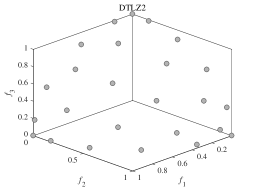
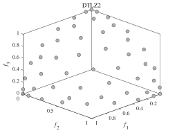
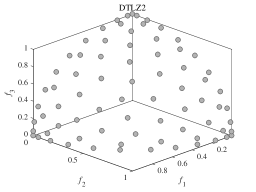
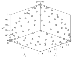
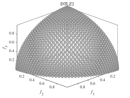
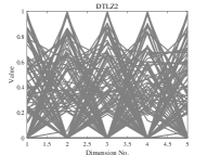
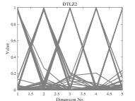
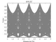
We now investigate the effectiveness of DPPs-Selection and whether it can maintain diversity. In order to show the diversity of the solutions chosen by DPPs-Selection, we carry out experiments on DTLZ2. We set the population sizes to 3, 25, 50, 75, and 100 and the number of function evaluations to 100’000. Figure 1 (a)-(e) shows the results of DPPs-Selection selecting 3, 25, 50, 75, and 100 solutions from a true PF, which is shown in Figure 1 (f). Regardless of the population size, MaOEADPPs maintains the diversity of the population. It can describe the distribution of true PF well with just a limited number of solutions.

To further evaluate the effectiveness of the DPPs-Selection, we replace it with $k$ -DPPs and uniform sampling. $k$ -DPPs selects eigenvectors based on the probability calculated by Equation (3) while DPPs-Selection selects the eigenvectors with $k$ largest eigenvalues.

We apply the modified algorithm to each instance independently for 30 times. We compare the experimental results of $k$ -DPPs, DPPs-Selection and uniform sampling on DTLZ1-DTLZ6 with 5, 10, 15 objectives. The population size is set to 126 for 5 objectives, 230 for 10 objectives, and 240 for 15 objectives. The number of function evaluations is set to 100’000.

The IGD values are shown in Table V. The experimental results demonstrate that DPPs-Selection outperforms the other methods on 14 of the 18 instances. This clearly indicates that is effective in selecting good offspring.

TABLE V: IGD VALUES OF DPPS-SELECTION,

k

-DPPS, AND UNIFORM SAMPLING ON DTLZ1-DTLZ6 WITH 5, 10 AND 15 OBJECTIVES. THE BEST RESULTS FOR EACH INSTANCE ARE HIGHLIGHTED IN GRAY.

Problem	$M$	$D$	DPPs-Selection	$k$ -DPPs	Uniform Sampling
DTLZ1	5	9	6.3302e-2 (2.01e-3) $+$	6.7296e-2 (1.50e-3) $+$	1.0132e-1 (3.60e-3)
DTLZ1	10	14	1.1160e-1 (7.24e-4) $+$	1.1097e-1 (1.41e-3) $+$	1.3398e-1 (3.13e-3)
DTLZ1	15	19	1.3144e-1 (2.25e-3) $+$	1.2933e-1 (3.66e-3) $+$	1.4420e-1 (3.78e-3)
DTLZ2	5	14	1.9256e-1 (9.47e-4) $+$	2.1073e-1 (2.27e-3) $+$	4.7890e-1 (1.76e-2)
DTLZ2	10	19	4.1889e-1 (3.08e-3) $+$	4.2137e-1 (2.30e-3) $+$	6.4167e-1 (1.04e-2)
DTLZ2	15	24	5.2576e-1 (2.53e-3) $+$	5.2848e-1 (2.48e-3) $+$	7.1932e-1 (1.42e-2)
DTLZ3	5	14	1.9863e-1 (3.76e-3) $+$	2.1074e-1 (3.26e-3) $+$	4.9174e-1 (1.57e-2)
DTLZ3	10	19	4.2238e-1 (7.54e-3) $+$	4.3082e-1 (1.58e-2) $+$	6.3344e-1 (1.65e-2)
DTLZ3	15	24	5.2696e-1 (5.94e-3) $+$	5.4254e-1 (1.76e-2) $+$	6.9256e-1 (1.95e-2)
DTLZ4	5	14	1.9286e-1 (9.25e-4) $+$	2.0636e-1 (2.29e-3) $+$	4.0326e-1 (5.62e-2)
DTLZ4	10	19	4.2837e-1 (2.71e-3) $+$	4.2613e-1 (1.70e-3) $+$	6.0528e-1 (1.35e-2)
DTLZ4	15	24	5.2782e-1 (9.74e-4) $+$	5.3930e-1 (2.47e-3) $+$	6.9463e-1 (1.45e-2)
DTLZ5	5	14	5.4818e-2 (3.13e-3) $+$	6.1737e-2 (1.11e-2) $+$	2.0254e-1 (4.49e-2)
DTLZ5	10	19	8.6127e-2 (9.47e-3) $+$	9.4108e-2 (1.49e-2) $+$	1.8816e-1 (3.92e-2)
DTLZ5	15	24	1.3073e-1 (1.76e-2) $+$	1.0559e-1 (1.33e-2) $+$	1.7968e-1 (2.09e-2)
DTLZ6	5	14	5.7469e-2 (3.00e-3) $+$	8.1320e-2 (1.26e-2) $+$	2.3739e-1 (3.75e-2)
DTLZ6	10	19	7.8330e-2 (9.20e-3) $+$	1.3341e-1 (3.87e-2) $+$	2.0934e-1 (4.00e-2)
DTLZ6	15	24	1.1411e-1 (1.48e-2) $+$	1.6549e-1 (4.05e-2) $\approx$	2.0659e-1 (3.55e-2)
$+/-/\approx$			18/0/0	17/0/1

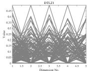
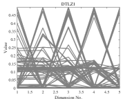
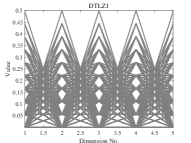
We now compare the distribution of the offspring obtained by DPPs-Selection and uniform sampling. We therefore run experiments on DTLZ1-DTLZ2 with 5 objectives. The population size is set to 126 and the number of function evaluations is 100’000. We perform 30 runs per instance. DPPs-Selection provides a uniform distribution of solutions, as shown in Figure 2. In contrast, the solutions from uniform sampling are clustered around several solutions.

IV-E Application Analysis

We now compare the CPU time of different algorithms and then investigate which types of problems MaOEADPPs is suitable for. We use instances of DTLZ1 to DTLZ8 with 5 and 10 objectives. The population size is set to 126 for 5 and to 230 for 10 objectives. The number of function evaluations is set to 100’000. We again perform 30 independent runs for each instance.

Table VI shows the consumed CPU time (measured in seconds) of MaOEADPPs and the other four algorithms. We can see that RVEA is the fastest. MaOEADPPs needs more time than RVEA, GrEA, RSEA, and NSGA-III, but less than AR-MOEA. The time complexity of MaOEADPPs is higher, but based on the excellent results discussed in the previous sections, this seems acceptable to us. Most of the computing time is spent on the eigen-decomposition.

TABLE VI: CPU TIME OF MAOEADPPS AND FOUR STATE-OF-THE-ART ALGORITHMS. THE BEST RESULTS FOR EACH INSTANCE ARE HIGHLIGHTED IN GRAY.

Problem	$M$	$D$	AR-MOEA	NSGA-III	RVEA	GrEA	MaOEADPPs
DTLZ1	5	9	6.5661e+1 (2.47e+0) $-$	3.8559e+0 (1.63e-1) $+$	2.7599e+0 (1.28e-1) $+$	4.2230e+1 (1.01e+0) $+$	5.4494e+1 (4.52e+0)
DTLZ1	10	14	3.3640e+2 (3.07e+1) $-$	5.8704e+0 (6.08e-1) $+$	2.7746e+0 (1.55e-1) $+$	1.1005e+2 (3.26e+0) $+$	1.6037e+2 (1.18e+1)
DTLZ2	5	14	1.0239e+2 (5.01e+0) $-$	4.1235e+0 (1.70e-1) $+$	2.9035e+0 (1.76e-1) $+$	5.5903e+1 (1.10e+0) $+$	6.0108e+1 (4.70e+0)
DTLZ2	10	19	4.5566e+2 (4.97e+1) $-$	5.9594e+0 (1.04e+0) $+$	2.9470e+0 (2.92e-1) $+$	1.1314e+2 (3.40e+0) $+$	2.0398e+2 (1.85e+1)
DTLZ3	5	14	5.6373e+1 (2.16e+0) $-$	4.0626e+0 (1.88e-1) $+$	2.9018e+0 (1.41e-1) $+$	3.7598e+1 (1.14e+0) $+$	4.6408e+1 (3.66e+0)
DTLZ3	10	19	3.2687e+2 (3.34e+1) $-$	6.1199e+0 (9.06e-1) $+$	2.8909e+0 (1.74e-1) $+$	1.0895e+2 (2.69e+0) $+$	1.5727e+2 (1.50e+1)
DTLZ4	5	14	1.0739e+2 (6.12e+0) $-$	4.6813e+0 (8.36e-1) $+$	2.9570e+0 (2.25e-1) $+$	5.7017e+1 (1.29e+0) $\approx$	6.0392e+1 (5.08e+0)
DTLZ4	10	19	4.6751e+2 (4.96e+1) $-$	5.8799e+0 (1.05e+0) $+$	3.0433e+0 (1.68e-1) $+$	1.1469e+2 (2.85e+0) $+$	2.0391e+2 (1.58e+1)
DTLZ5	5	14	1.0600e+2 (4.72e+0) $-$	6.2078e+0 (3.72e-1) $+$	2.3133e+0 (1.82e-1) $+$	6.1369e+1 (1.36e+0) $+$	6.8480e+1 (6.22e+0)
DTLZ5	10	19	4.3173e+2 (3.84e+1) $-$	7.6929e+0 (8.37e-1) $+$	2.3730e+0 (1.32e-1) $+$	1.1278e+2 (2.89e+0) $+$	1.9501e+2 (1.44e+1)
DTLZ6	5	14	9.4896e+1 (4.01e+0) $-$	5.8468e+0 (3.78e-1) $+$	2.7999e+0 (2.08e-1) $+$	5.6629e+1 (1.52e+0) $+$	6.1332e+1 (4.61e+0)
DTLZ6	10	19	4.0879e+2 (3.60e+1) $-$	7.2795e+0 (9.04e-1) $+$	2.7355e+0 (1.78e-1) $+$	1.1106e+2 (2.98e+0) $+$	1.6366e+2 (1.07e+1)
DTLZ7	5	24	1.0802e+2 (5.21e+0) $-$	6.7572e+0 (5.06e-1) $+$	2.4925e+0 (1.70e-1) $+$	5.7722e+1 (1.42e+0) $+$	6.7323e+1 (4.35e+0)
DTLZ7	10	29	4.9773e+2 (4.66e+1) $-$	7.4693e+0 (6.19e-1) $+$	2.3939e+0 (2.86e-1) $+$	1.1469e+2 (3.21e+0) $+$	2.1071e+2 (1.67e+1)
DTLZ8	5	50	6.6489e+1 (4.64e+0) $-$	6.6228e+0 (7.32e-1) $+$	3.2762e+0 (2.31e-1) $+$	4.0555e+1 (1.79e+0) $+$	4.2583e+1 (4.39e+0)
DTLZ8	10	100	2.7658e+2 (1.47e+1) $-$	8.5522e+0 (8.12e-1) $+$	3.8377e+0 (2.41e-1) $+$	1.2365e+2 (4.54e+0) $+$	1.8164e+2 (7.85e+0)

TABLE VII: IGD VALUES OBTAINED BY MAOEADPPS, AR-MOEA [39], NSGA-III [36], RSEA [37],

\theta

-DEA [38], AND RVEA [40] ON DTLZ1-DTLZ4, IDTLZ1-IDTLZ2, AND WFG1-WFG9 WITH 20, 25 AND 30 OBJECTIVES. THE BEST RESULTS FOR EACH INSTANCE ARE HIGHLIGHTED IN GRAY.

Problem	$M$	$D$	MaOEADPPs	AR-MOEA	NSGA-III	RSEA	$\theta$ -DEA	RVEA
DTLZ1	20	24	1.6935e-1 (5.89e-3)	1.8317e-1 (5.37e-3) $-$	2.0905e-1 (2.76e-2) $-$	2.5023e-1 (2.39e-2) $-$	2.4336e-1 (2.55e-2) $-$	1.7192e-1 (4.52e-3) $\approx$
DTLZ1	25	29	1.5989e-1 (5.78e-3)	2.0995e-1 (1.25e-2) $-$	3.4554e-1 (1.10e-1) $-$	2.5450e-1 (4.56e-2) $-$	3.0196e-1 (3.34e-2) $-$	1.8809e-1 (1.26e-2) $-$
DTLZ1	30	34	1.7267e-1 (2.88e-3)	2.0919e-1 (6.88e-3) $-$	2.8360e-1 (2.07e-2) $-$	2.2535e-1 (2.71e-2) $-$	3.1785e-1 (4.84e-2) $-$	1.9325e-1 (6.34e-3) $-$
DTLZ2	20	29	5.8814e-1 (1.44e-3)	6.2045e-1 (1.18e-3) $-$	7.5759e-1 (4.03e-2) $-$	7.3204e-1 (2.25e-2) $-$	6.2287e-1 (2.65e-4) $-$	6.4054e-1 (3.92e-2) $-$
DTLZ2	25	34	5.6679e-1 (1.08e-3)	7.9821e-1 (2.37e-2) $-$	9.8159e-1 (2.44e-2) $-$	7.6549e-1 (2.13e-2) $-$	8.0077e-1 (2.64e-2) $-$	1.1378e+0 (1.33e-1) $-$
DTLZ2	30	39	5.7159e-1 (2.15e-3)	8.4406e-1 (2.54e-2) $-$	8.5350e-1 (9.35e-3) $-$	8.0201e-1 (3.75e-2) $-$	8.3091e-1 (1.29e-2) $-$	1.2173e+0 (1.48e-1) $-$
DTLZ3	20	29	6.3938e-1 (2.58e-2)	6.3548e-1 (2.40e-2) $\approx$	5.8748e+1 (3.19e+1) $-$	2.0867e+0 (1.36e+0) $-$	8.7577e-1 (3.31e-1) $-$	6.4834e-1 (1.99e-2) $\approx$
DTLZ3	25	34	6.9541e-1 (5.33e-2)	9.1638e-1 (9.02e-2) $-$	4.4350e+0 (2.58e+0) $-$	3.4304e+0 (1.90e+0) $-$	1.3322e+0 (5.65e-1) $-$	1.1717e+0 (1.88e-1) $-$
DTLZ3	30	39	9.1521e-1 (5.59e-2)	9.4735e-1 (4.23e-2) $\approx$	1.9279e+0 (1.37e+0) $-$	4.7211e+0 (2.99e+0) $-$	1.2745e+0 (3.52e-1) $-$	1.1657e+0 (1.22e-1) $-$
DTLZ4	20	29	5.8886e-1 (1.26e-3)	6.1904e-1 (6.32e-4) $-$	6.8387e-1 (5.20e-2) $-$	7.1766e-1 (1.34e-2) $-$	6.2301e-1 (5.88e-5) $-$	6.2318e-1 (7.11e-5) $-$
DTLZ4	25	34	5.7182e-1 (4.78e-4)	7.9480e-1 (5.26e-3) $-$	9.6287e-1 (3.85e-2) $-$	7.6557e-1 (1.67e-2) $-$	7.7492e-1 (1.29e-3) $-$	8.2984e-1 (2.57e-2) $-$
DTLZ4	30	39	5.8104e-1 (5.87e-4)	8.1673e-1 (3.02e-3) $-$	8.5469e-1 (1.01e-2) $-$	8.1422e-1 (1.09e-2) $-$	8.0093e-1 (1.30e-3) $-$	8.2006e-1 (2.23e-3) $-$
IDTLZ1	20	24	1.7950e-1 (3.48e-3)	2.0867e-1 (1.70e-2) $-$	2.2502e-1 (1.07e-2) $-$	2.1841e-1 (1.00e-2) $-$	2.3480e-1 (8.83e-3) $-$	3.9018e-1 (3.56e-2) $-$
IDTLZ1	25	29	1.7689e-1 (6.70e-3)	2.5662e-1 (1.58e-2) $-$	2.2169e-1 (4.88e-3) $-$	2.1581e-1 (8.49e-3) $-$	2.1597e-1 (5.56e-3) $-$	3.6129e-1 (4.53e-2) $-$
IDTLZ1	30	34	1.8500e-1 (7.06e-3)	2.5841e-1 (1.41e-2) $-$	2.2867e-1 (4.67e-3) $-$	2.2556e-1 (8.28e-3) $-$	2.1883e-1 (5.43e-3) $-$	4.0375e-1 (4.15e-2) $-$
IDTLZ2	20	29	6.0817e-1 (2.84e-3)	7.5260e-1 (1.40e-2) $-$	8.2186e-1 (1.47e-2) $-$	8.9332e-1 (8.68e-3) $-$	1.0703e+0 (4.38e-3) $-$	1.0573e+0 (6.83e-3) $-$
IDTLZ2	25	34	5.6219e-1 (2.99e-3)	8.8987e-1 (3.19e-2) $-$	9.4107e-1 (3.26e-2) $-$	8.8319e-1 (8.75e-3) $-$	1.0284e+0 (9.56e-3) $-$	1.1280e+0 (1.61e-2) $-$
IDTLZ2	30	39	5.7035e-1 (2.15e-3)	9.4525e-1 (4.04e-2) $-$	9.5061e-1 (6.20e-2) $-$	9.3419e-1 (3.32e-3) $-$	9.8636e-1 (8.10e-2) $-$	1.1657e+0 (5.73e-3) $-$
WFG1	20	29	2.8416e+0 (5.71e-2)	4.3317e+0 (1.07e-1) $-$	4.5705e+0 (2.50e-1) $-$	3.3638e+0 (7.35e-2) $-$	3.8257e+0 (1.55e-1) $-$	3.9325e+0 (8.88e-2) $-$
WFG1	25	34	2.6685e+0 (1.38e-1)	4.3395e+0 (4.52e-2) $-$	4.6421e+0 (1.74e-1) $-$	3.2426e+0 (1.57e-1) $-$	4.1055e+0 (1.24e-1) $-$	4.2723e+0 (7.51e-2) $-$
WFG1	30	39	3.1385e+0 (6.05e-2)	5.0391e+0 (7.49e-2) $-$	5.0819e+0 (3.44e-1) $-$	4.0689e+0 (2.29e-1) $-$	4.8393e+0 (1.43e-1) $-$	4.8916e+0 (9.55e-2) $-$
WFG2	20	29	2.7857e+0 (5.94e-2)	3.3199e+0 (1.81e-1) $-$	4.0051e+0 (1.70e-1) $-$	4.2709e+0 (4.71e-1) $-$	8.3963e+0 (2.41e-1) $-$	3.3546e+0 (1.54e-1) $-$
WFG2	25	34	2.5679e+0 (9.42e-2)	3.4314e+0 (1.50e-1) $-$	7.7962e+0 (2.91e+0) $-$	5.5383e+0 (1.36e+0) $-$	1.4250e+1 (2.86e+0) $-$	4.2759e+0 (8.53e-2) $-$
WFG2	30	39	2.9826e+0 (8.56e-2)	4.1345e+0 (1.51e-1) $-$	4.7334e+0 (4.81e-1) $-$	6.4618e+0 (1.45e+0) $-$	1.7321e+1 (4.11e+0) $-$	4.7467e+0 (1.37e-1) $-$
WFG3	20	29	3.8937e+0 (3.58e-1)	7.6670e+0 (2.35e-1) $-$	8.9111e+0 (2.21e+0) $-$	3.6430e+0 (2.10e+0) $\approx$	2.8643e+0 (2.48e-1) $+$	1.0329e+1 (3.05e+0) $-$
WFG3	25	34	5.0618e+0 (7.49e-1)	9.9951e+0 (1.63e+0) $-$	1.8565e+1 (4.36e+0) $-$	7.1375e+0 (3.62e+0) $-$	8.0814e+0 (9.90e-1) $-$	1.5028e+1 (2.84e+0) $-$
WFG3	30	39	4.5820e+0 (7.64e-1)	1.2189e+1 (1.97e+0) $-$	8.9821e+0 (1.58e+0) $-$	4.1652e+0 (2.67e+0) $\approx$	9.5068e+0 (1.14e+0) $-$	1.7722e+1 (1.14e+0) $-$
WFG4	20	29	1.0771e+1 (1.46e-1)	1.1501e+1 (4.03e-2) $-$	1.2316e+1 (6.83e-1) $-$	1.3459e+1 (3.95e-1) $-$	1.1459e+1 (1.26e-2) $-$	1.2430e+1 (3.98e-1) $-$
WFG4	25	34	1.1448e+1 (7.12e-2)	2.2522e+1 (1.43e+0) $-$	2.0519e+1 (8.80e-1) $-$	1.8238e+1 (5.28e-1) $-$	2.1231e+1 (2.50e-1) $-$	2.1083e+1 (9.00e-1) $-$
WFG4	30	39	1.4064e+1 (3.89e-1)	2.9242e+1 (1.40e+0) $-$	2.5464e+1 (2.70e-1) $-$	2.2991e+1 (3.21e-1) $-$	2.6360e+1 (2.48e-1) $-$	2.5982e+1 (2.98e-1) $-$
WFG5	20	29	1.0807e+1 (3.45e-2)	1.1498e+1 (2.51e-2) $-$	1.1919e+1 (8.91e-1) $-$	1.3100e+1 (2.55e-1) $-$	1.1311e+1 (6.55e-2) $-$	1.1781e+1 (9.05e-2) $-$
WFG5	25	34	1.1298e+1 (3.73e-2)	2.0772e+1 (7.94e-1) $-$	2.0517e+1 (6.45e-1) $-$	1.6908e+1 (3.24e-1) $-$	2.0838e+1 (3.52e-1) $-$	2.1135e+1 (1.02e+0) $-$
WFG5	30	39	1.3500e+1 (1.68e-1)	2.7843e+1 (2.48e+0) $-$	2.5424e+1 (1.85e-1) $-$	2.1837e+1 (6.32e-1) $-$	2.5355e+1 (2.20e-1) $-$	2.6277e+1 (6.84e-1) $-$
WFG6	20	29	1.0545e+1 (2.04e-1)	1.1564e+1 (2.40e-2) $-$	1.4251e+1 (7.35e-1) $-$	1.4219e+1 (3.13e-1) $-$	1.1519e+1 (1.77e-2) $-$	1.3099e+1 (2.28e-1) $-$
WFG6	25	34	1.1426e+1 (6.55e-2)	2.2205e+1 (1.01e+0) $-$	2.1670e+1 (9.75e-1) $-$	1.9284e+1 (9.24e-1) $-$	2.1142e+1 (2.76e-1) $-$	2.4464e+1 (2.98e+0) $-$
WFG6	30	39	1.3568e+1 (4.89e-2)	2.7633e+1 (1.42e+0) $-$	2.5705e+1 (7.05e-1) $-$	2.4238e+1 (1.02e+0) $-$	2.5888e+1 (3.09e-1) $-$	3.0529e+1 (1.93e+0) $-$
WFG7	20	29	1.0701e+1 (5.17e-2)	1.1652e+1 (4.25e-2) $-$	1.4793e+1 (9.31e-1) $-$	1.4335e+1 (5.76e-1) $-$	1.1494e+1 (4.67e-2) $-$	1.1831e+1 (3.53e-1) $-$
WFG7	25	34	1.1613e+1 (8.21e-2)	2.2584e+1 (7.95e-1) $-$	2.0911e+1 (1.06e+0) $-$	1.9592e+1 (1.15e+0) $-$	2.1747e+1 (7.73e-1) $-$	2.7103e+1 (1.06e+1) $-$
WFG7	30	39	1.4747e+1 (2.94e-1)	2.9547e+1 (9.79e-1) $-$	2.5760e+1 (6.03e-2) $-$	2.5355e+1 (1.04e+0) $-$	2.6840e+1 (6.37e-1) $-$	2.7464e+1 (1.68e+0) $-$
WFG8	20	29	1.0602e+1 (1.27e-1)	1.1549e+1 (2.23e-2) $-$	1.3472e+1 (1.37e+0) $-$	1.6935e+1 (4.24e-1) $-$	1.2782e+1 (3.53e-1) $-$	1.2662e+1 (7.01e-1) $-$
WFG8	25	34	1.3453e+1 (1.61e+0)	2.3285e+1 (1.02e+0) $-$	2.2056e+1 (1.86e+0) $-$	2.2662e+1 (6.99e-1) $-$	2.1532e+1 (6.84e-1) $-$	2.6385e+1 (7.50e+0) $-$
WFG8	30	39	1.6808e+1 (2.42e+0)	3.1358e+1 (8.10e-1) $-$	2.6514e+1 (2.87e-1) $-$	2.9600e+1 (8.20e-1) $-$	2.7165e+1 (5.15e-1) $-$	2.9285e+1 (3.28e+0) $-$
WFG9	20	29	1.0970e+1 (1.34e-1)	1.1725e+1 (1.07e-1) $-$	1.3277e+1 (1.49e+0) $-$	1.3659e+1 (3.04e-1) $-$	1.1386e+1 (2.58e-1) $-$	1.1674e+1 (3.53e-1) $-$
WFG9	25	34	1.2027e+1 (5.54e-1)	2.2138e+1 (6.15e-1) $-$	2.0130e+1 (4.52e-1) $-$	1.7073e+1 (3.48e-1) $-$	2.0740e+1 (2.10e-1) $-$	2.1086e+1 (1.52e+0) $-$
WFG9	30	39	1.5320e+1 (7.84e-1)	2.9121e+1 (9.59e-1) $-$	2.5257e+1 (7.76e-1) $-$	2.1094e+1 (6.04e-1) $-$	2.5459e+1 (3.21e-1) $-$	2.5826e+1 (2.89e+0) $-$
$+/-/\approx$				0/43/2	0/45/0	0/43/2	1/44/0	0/43/2

We believe that MaOEADPPs is suitable for solving problems which are not time critical but sufficiently difficult. From another perspective, it is also suitable for problems where the objective function evaluations are time consuming, because in this case, the runtime requirements of MaOEADPPs will not play an important role. For example, many application scenarios such as engineering design optimization, damage detection and pipeline systems [47] have a large number of decision variables. These applications usually do not require very quick responses but improvements of solution quality can have a positive impact.

We thus compare our MaOEADPPs with the other algorithms on the 8 large-scale instances LSMOP1 to LSMOP5, MONRP, SMOP1 and MOKP with 5 or 2 objectives. We again perform 30 independent runs per instance. The population size is 126 and the number of function evaluations is set to 100’000. As shown in Table VIII, MaOEADPPs obtains the best IGD values on 6 of the 8 instances.

MaOEADPPs is also suitable for problems with a large number of objectives. To verify this, we carry out comparison experiments on DTLZ1-DTLZ4, WFG1-WFG9 and IDTLZ1-IDTLZ2 with 20, 25 and 30 objectives. We perform again 30 independent runs per instance. We set the population size to 400 for instances with 30 objectives and to 300 for instances with 20 and 25 objectives. The number of function evaluations is set to 100’000.

As shown in Table VII, our MaOEADPPs returns the best results on 42 of the 45 instances. Moreover, as the number of objectives increases, the gaps between the IGD values of our MaOEADPPs and the compared algorithms gradually widen. One possible reason is that MaOEADPPs uses the Kernel Matrix $\boldsymbol{L}$ to measure the convergence and similarity between solution pairs, which reflects more details of the distribution in the population.

TABLE VIII: IGD VALUES OF AR-MOEA [39], NSGA-III [36], RSEA [37] AND

\theta

-DEA [38] ON PROBLEMS WITH A LARGE NUMBER OF DECISION VARIABLES. THE BEST RESULTS FOR EACH INSTANCE ARE HIGHLIGHTED IN GRAY.

Problem	$M$	$D$	MaOEADPPs	AR-MOEA	NSGA-III	$\theta-$ DEA	RSEA
SMOP1	5	100	1.2944e-1 (1.30e-3)	1.3449e-1 (1.69e-3) $-$	1.3601e-1 (2.19e-3) $-$	1.3093e-1 (1.66e-3) $-$	1.5153e-1 (3.75e-3) $-$
MOKP	5	250	1.7386e+4 (2.25e+2)	1.7528e+4 (9.28e+1) $-$	1.7168e+4 (1.62e+2) $+$	1.7337e+4 (1.12e+2) $\approx$	1.7526e+4 (1.12e+2) $-$
MONRP	2	100	2.7285e+3 (5.82e+2)	8.9542e+3 (1.26e+3) $-$	7.6479e+3 (7.22e+2) $-$	8.4295e+3 (9.67e+2) $-$	9.9819e+3 (1.08e+3) $-$
LSMOP1	5	500	1.4587e+0 (1.97e-1)	3.8753e+0 (4.51e-1) $-$	3.3043e+0 (4.01e-1) $-$	9.0859e-1 (8.97e-2) $+$	7.8286e-1 (1.10e-1) $+$
LSMOP2	5	500	1.6795e-1 (1.03e-3)	1.7401e-1 (4.16e-4) $-$	1.7492e-1 (7.40e-4) $-$	1.7411e-1 (6.70e-4) $-$	1.8579e-1 (3.41e-3) $-$
LSMOP3	5	500	5.2013e+0 (7.16e-1)	7.7309e+0 (1.08e+0) $-$	9.5593e+0 (1.42e+0) $-$	9.8999e+0 (3.24e+0) $-$	9.2354e+0 (2.28e+0) $-$
LSMOP4	5	500	2.8271e-1 (5.33e-3)	3.0373e-1 (4.04e-3) $-$	3.0943e-1 (5.85e-3) $-$	2.9601e-1 (4.46e-3) $-$	2.9578e-1 (1.52e-2) $-$
LSMOP5	5	500	2.1142e+0 (7.12e-1)	3.4117e+0 (9.69e-1) $-$	6.9847e+0 (7.16e-1) $-$	4.7954e+0 (5.67e-1) $-$	3.6352e+0 (6.41e-1) $-$
$+/-/\approx$				0/8/0	1/7/0	1/6/1	1/7/0

V CONCLUSION

In this paper, we propose a new MaOEA named MaOEADPPs. We show that the algorithm is suitable for solving a variety of types of MaOPs. For MaOEADPPs, we design the new Determinantal Point Processes Selection (DPPs-Selection) method for the Environmental Selection. In order to adapt to various types of MaOPs, a Kernel Matrix is defined. We compare MaOEADPPs with several state-of-the-art algorithms on the DTLZ, WFG, and MaF benchmarks with the number of objectives ranging from 5 to 30. The experimental results demonstrate that our MaOEADPPs significantly outperforms the other algorithms. We find that the Kernel Matrix of MaOEADPPs can adapt to problems with different objective types. Our results also suggest that MaOEADPPs is not the fastest algorithm but also not slow. It is therefore suitable for solving problems where the objective function evaluations are time consuming or which are not time critical. The Kernel Matrix of the DPPs-Selection is the key component of our MaOEADPPs. We will try to further improve it in the future work and especially focus on investigating alternative definitions for the solutions quality metrics.

ACKNOWLEDGEMENT

This research work was supported by the National Natural Science Foundation of China under Grant 61573328.

References

[1] H. Chen and X. Yao, “Multiobjective neural network ensembles based on regularized negative correlation learning,” IEEE Transactions on Knowledge and Data Engineering, vol. 22, no. 12, pp. 1738–1751, 2010.
[2] H. Chen and X. Yao, “Evolutionary random neural ensembles based on negative correlation learning,” in IEEE Congress on Evolutionary Computation, 2007, pp. 130–141.
[3] P. J. Fleming, R. C. Purshouse, and R. J. Lygoe, “Many-objective optimization: An engineering design perspective,” 2005.
[4] Z. Gong, H. Chen, B. Yuan, and X. Yao, “Multiobjective learning in the model space for time series classification,” IEEE Transactions on Cybernetics, vol. PP, no. 3, pp. 1–15, 2018.
[5] B. Li, J. Li, K. Tang, and X. Yao, “Many-objective evolutionary algorithms: A survey,” ACM Computing Surveys (CSUR), vol. 48, no. 1, p. 13, 2015.
[6] Fonseca, Carlos, M., Fleming, Peter, and J., “Multiobjective optimization and multiple constraint handling with evolutionary algorithms-part i…” IEEE Transactions on Systems, Man And Cybernetics: Part A, 1998.
[7] D. Hadka and P. Reed, “Borg: An auto-adaptive many-objective evolutionary computing framework,” Evolutionary Computation, vol. 21, no. 2, pp. 231–259, 2013.
[8] Z. He, G. G. Yen, and J. Zhang, “Fuzzy-based Pareto optimality for many-objective evolutionary algorithms,” IEEE Transactions on Evolutionary Computation, vol. 18, no. 2, pp. 269–285, 2014.
[9] R. Tanabe, H. Ishibuchi, A. Oyama, R. Tanabe, H. Ishibuchi, and A. Oyama, “Benchmarking multi- and many-objective evolutionary algorithms under two optimization scenarios,” IEEE Access, vol. 5, no. 99, pp. 19 597–19 619, 2017.
[10] H. K. Singh, K. S. Bhattacharjee, and T. Ray, “Distance-based subset selection for benchmarking in evolutionary multi/many-objective optimization,” IEEE Transactions on Evolutionary Computation, vol. 23, no. 5, pp. 904–912, 2019.
[11] X. Zhang, Y. Tian, and Y. Jin, “A knee point-driven evolutionary algorithm for many-objective optimization,” IEEE Transactions on Evolutionary Computation, vol. 19, no. 6, pp. 761–776, 2015.
[12] M. Li, S. Yang, and X. Liu, “Shift-based density estimation for Pareto-based algorithms in many-objective optimization,” IEEE Transactions on Evolutionary Computation, vol. 18, no. 3, pp. 348–365, 2014.
[13] L. While, P. Hingston, L. Barone, and S. Huband, “A faster algorithm for calculating hypervolume,” IEEE Transactions on Evolutionary Computation, vol. 10, no. 1, pp. 29–38, 2006.
[14] M. Emmerich, N. Beume, and B. Naujoks, “An EMO algorithm using the hypervolume measure as selection criterion,” in Evolutionary Multi-Criterion Optimization, 2005, pp. 62–76.
[15] J. Bader and E. Zitzler, “HypE: An algorithm for fast hypervolume-based many-objective optimization,” Evolutionary computation, vol. 19, no. 1, pp. 45–76, 2011.
[16] D. Brockhoff, T. Wagner, and H. Trautmann, “On the properties of the r2 indicator,” ser. GECCO 2012, 2012, p. 465–472.
[17] P. A. N. Bosman and D. Thierens, “The balance between proximity and diversity in multiobjective evolutionary algorithms,” Evolutionary Computation IEEE Transactions on, vol. 7, no. 2, pp. 174–188, 2003.
[18] R. H. Gómez and C. A. C. Coello, “Mombi: A new metaheuristic for many-objective optimization based on the r2 indicator,” in 2013 IEEE Congress on Evolutionary Computation, 2013, pp. 2488–2495.
[19] R. Denysiuk, L. Costa, and I. E. Santo, “Many-objective optimization using differential evolution with variable-wise mutation restriction,” in Genetic and Evolutionary Computation Conference, 2013.
[20] E. Zitzler and S. Künzli, “Indicator-based selection in multiobjective search,” in International Conference on Parallel Problem Solving from Nature, 2004.
[21] R. Cheng, Y. Jin, M. Olhofer, and B. Sendhoff, “A reference vector guided evolutionary algorithm for many-objective optimization,” IEEE Transactions on Evolutionary Computation, vol. 20, no. 5, 2016.
[22] Q. Zhang and H. Li, “MOEA/D: A multiobjective evolutionary algorithm based on decomposition,” IEEE Transactions on Evolutionary Computation, vol. 11, no. 6, pp. 712–731, 2007.
[23] Fellow, IEEE, H. Jain, and K. Deb, “An evolutionary many-objective optimization algorithm using reference-point based nondominated sorting approach, part ii: Handling constraints and extending to an adaptive approach,” IEEE Transactions on Evolutionary Computation, vol. 18, no. 4, pp. 602–622, 2014.
[24] S. Jiang and S. Yang, “A strength pareto evolutionary algorithm based on reference direction for multi-objective and many-objective optimization,” IEEE Transactions on Evolutionary Computation, pp. 329–346, 2017.
[25] B. Li, J. Li, K. Tang, and X. Yao, “Many-objective evolutionary algorithms: A survey,” ACM Comput. Surv., vol. 48, no. 1, 2015.
[26] S. Zapotecas-Martínez, C. A. Coello Coello, H. E. Aguirre, and K. Tanaka, “A review of features and limitations of existing scalable multiobjective test suites,” IEEE Transactions on Evolutionary Computation, vol. 23, no. 1, pp. 130–142, 2019.
[27] H. K. Singh, A. Isaacs, and T. Ray, “A pareto corner search evolutionary algorithm and dimensionality reduction in many-objective optimization problems,” IEEE Transactions on Evolutionary Computation, vol. 15, no. 4, pp. 539–556, 2011.
[28] M. Gartrell, U. Paquet, and N. Koenigstein, “Bayesian low-rank determinantal point processes,” in Proceedings of the 10th ACM Conference on Recommender Systems, 2016, p. 349–356.
[29] A. Kulesza, B. Taskar et al., “Determinantal point processes for machine learning,” Foundations and Trends® in Machine Learning, vol. 5, no. 2–3, pp. 123–286, 2012.
[30] A. Kulesza and B. Taskar, “k-DPPs: Fixed-size determinantal point processes,” in Proceedings of the 28th International Conference on Machine Learning, 2011, pp. 1193–1200.
[31] N. Tremblay, P.-O. Amblard, and S. Barthelmé, “Graph sampling with determinantal processes,” in European Signal Processing Conference, 2017, pp. 1674–1678.
[32] C. Ran, M. Li, T. Ye, X. Zhang, S. Yang, Y. Jin, and Y. Xin, “A benchmark test suite for evolutionary many-objective optimization,” Complex & Intelligent Systems, vol. 3, no. 1, pp. 67–81, 2017.
[33] H. Ishibuchi, S. Yu, H. Masuda, and Y. Nojima, “Performance of decomposition-based many-objective algorithms strongly depends on pareto front shapes,” IEEE Transactions on Evolutionary Computation, vol. 21, no. 2, pp. 169–190, 2017.
[34] R. B. Agrawal, K. Deb, and R. Agrawal, “Simulated binary crossover for continuous search space,” Complex Systems, vol. 9, no. 2, pp. 115–148, 1995.
[35] K. Deb and M. Goyal, “A combined genetic adaptive search (GeneAS) for engineering design,” Computer Science and Informatics, vol. 26, pp. 30–45, 1996.
[36] K. Deb and H. Jain, “An evolutionary many-objective optimization algorithm using reference-point-based nondominated sorting approach, part I: Solving problems with box constraints.” IEEE Transactions Evolutionary Computation, vol. 18, no. 4, pp. 577–601, 2014.
[37] C. He, Y. Tian, Y. Jin, X. Zhang, and L. Pan, “A radial space division based evolutionary algorithm for many-objective optimization,” Applied Soft Computing, vol. 61, pp. 603–621, 2017.
[38] Y. Yuan, H. Xu, B. Wang, and X. Yao, “A new dominance relation-based evolutionary algorithm for many-objective optimization,” IEEE Transactions on Evolutionary Computation, vol. 20, no. 1, pp. 16–37, 2016.
[39] Y. Tian, R. Cheng, X. Zhang, F. Cheng, and Y. Jin, “An indicator based multi-objective evolutionary algorithm with reference point adaptation for better versatility,” IEEE Transactions on Evolutionary Computation, vol. PP, no. 99, pp. 1–1, 2017.
[40] R. Cheng, Y. Jin, M. Olhofer, and B. Sendhoff, “A reference vector guided evolutionary algorithm for many-objective optimization,” IEEE Transactions on Evolutionary Computation, vol. 20, no. 5, pp. 773–791, 2016.
[41] Y. Tian, R. Cheng, X. Zhang, and Y. Jin, “PlatEMO: A MATLAB platform for evolutionary multi-objective optimization,” IEEE Computational Intelligence Magazine, vol. 12, no. 4, pp. 73–87, 2017.
[42] K. Deb, L. Thiele, M. Laumanns, and E. Zitzler, “Scalable test problems for evolutionary multiobjective optimization,” in Evolutionary Multiobjective Optimization, 2005, pp. 105–145.
[43] H. Jain and K. Deb, “An evolutionary many-objective optimization algorithm using reference-point based nondominated sorting approach, Part II: Handling constraints and extending to an adaptive approach.” IEEE Transactions Evolutionary Computation, vol. 18, no. 4, pp. 602–622, 2014.
[44] S. Huband, P. Hingston, L. Barone, and L. While, “A review of multiobjective test problems and a scalable test problem toolkit,” IEEE Transactions on Evolutionary Computation, vol. 10, no. 5, pp. 477–506, 2006.
[45] A. Zhou, Y. Jin, Q. Zhang, B. Sendhoff, and E. Tsang, “Combining model-based and genetics-based offspring generation for multi-objective optimization using a convergence criterion,” in Proceedings of the IEEE Congress on Evolutionary Computation, 2006, pp. 892–899.
[46] I. Das and J. E. Dennis, “Normal-boundary intersection: A new method for generating the Pareto surface in nonlinear multicriteria optimization problems,” SIAM Journal on Optimization, vol. 8, no. 3, pp. 631–657, 1998.
[47] S. Mahdavi, M. E. Shiri, and S. Rahnamayan, “Metaheuristics in large-scale global continues optimization: A survey,” Information Sciences, vol. 295, pp. 407–428, 2015.