A new method for deriving composition of S-type asteroids from noisy and incomplete near-infrared spectra
Abstract
The surface composition of S-type asteroids can be determined using band parameters extracted from their near-infrared (NIR) spectra (0.7-2.50 m) along with spectral calibrations derived from laboratory samples. In the past, these empirical equations have been obtained by combining NIR spectra of meteorite samples with information about their composition and mineral abundance. For these equations to give accurate results, the characteristics of the laboratory spectra they are derived from should be similar to those of asteroid spectral data (i.e., similar signal-to-noise ratio (S/N) and wavelength range). Here we present new spectral calibrations that can be used to determine the mineral composition of ordinary chondrite-like S-type asteroids. Contrary to previous work, the S/N of the ordinary chondrite spectra used in this study has been decreased to recreate the S/N typically observed among asteroid spectra, allowing us to obtain more realistic results. In addition, the new equations have been derived for five wavelength ranges encompassed between 0.7 and 2.50 m, making it possible to determine the composition of asteroids with incomplete data. The new spectral calibrations were tested using band parameters measured from the NIR spectrum of asteroid (25143) Itokawa, and comparing the results with laboratory measurements of the returned samples. We found that the spectrally derived olivine and pyroxene chemistry, which are given by the molar contents of fayalite (Fa) and ferrosilite (Fs), are in excellent agreement with the mean values measured from the samples (Fa28.6±1.1 and Fs23.1±2.2), with a maximum difference of 0.6 mol% for Fa and 1.4 mol% for Fs.
1 Introduction
Understanding the compositions of asteroids is crucial to answering important questions regarding solar system formation and evolution. Due to our ability to remotely determine the compositions of many asteroids, studies can span from detailed investigations of individual objects to questions regarding the compositional distribution of asteroids throughout the solar system. To determine the compositions of asteroids, researchers seek diagnostic spectral band parameters, which enable them to investigate their mineralogies remotely using telescopes.
For objects belonging to the S, Q, and V classes, which show prominent 1 and 2 m absorption features, spectral band parameters such as band centers can be used to determine a more precise composition than taxonomy alone provides (e.g., Burns et al., 1972; Adams, 1974; Gaffey et al., 1993; Sanchez et al., 2012; Dunn et al., 2013; Thomas et al., 2014). These diagnostic absorption features are indicative of crystalline olivine ((Mg, Fe)2SiO4) and/or pyroxene ((Mg, Fe)2Si2O6). Olivine characteristically shows a broad absorption feature centered near 1.04-1.1 m that is comprised of three overlapping bands, while pyroxenes show two broad absorption features centered at 0.9-1 m and 1.9-2 m. For olivine-pyroxene mixtures, the wavelength of the 1 m feature (Band I, BI) is a function of the relative abundances and compositions of olivine and pyroxene, while the wavelength of the 2 m feature (Band II, BII) is a function of the pyroxene composition (e.g., Cloutis et al., 1986). The ratio of the area of Band II to Band I, or band area ratio (BAR), is also a measure of the relative abundances of olivine and pyroxene.
The relationships between band parameters and mineralogical composition can be rigorously calculated for various types of meteorites, including ordinary chondrites (Gaffey et al., 2002; Dunn et al., 2010a), olivine-dominated meteorites (Sanchez et al., 2014), primitive achondrites (Lucas et al., 2019), and basaltic achondrites (Burbine et al., 2009, 2018). Dunn et al. (2010a, b, c) used a combination of band parameters from laboratory spectra of meteorites, measured mineral abundances from x-ray diffraction (XRD), and mafic silicate compositions determined from electron microprobe analysis to formulate the mathematical relationships between band parameters and composition for ordinary chondrite meteorites. These quantitative relationships can be applied to asteroids whose spectra are similar to ordinary chondrites (e.g., the S(IV) region defined by Gaffey et al., 1993).
The current method of determining the composition of ordinary chondrite-like asteroids depends on these laboratory studies that correlate meteorite mineralogies with spectral band parameters from high signal-to-noise ratio (S/N) laboratory spectra. The accuracy and precision of any given calculation of asteroid composition depends greatly on the S/N of the observed asteroid spectrum and the researcher’s ability to duplicate the methodology with which band parameters are determined. Many works (e.g., Sanchez et al., 2012; Thomas et al., 2014) also incorporate corrections for temperature and phase angle of the asteroid during observation to adjust the band parameters such that they match the conditions of the laboratory measurements.
There are several factors that hinder our ability to accurately apply these derived mineralogical relationships to near-infrared (NIR) spectra of asteroids. The use of a dichroic filter in an NIR spectrograph can exclude the local maximum at 0.74 m that is used to define the continuum for Band I. In the past, these observations have been complemented by visible wavelength spectra (0.4-0.9 m) from legacy surveys such as SMASS (e.g., Xu et al., 1995; Bus, & Binzel, 2002). However, the majority of new asteroid spectral observations in the last two decades are only in NIR wavelengths. Noise from incomplete correction of telluric bands at 1.8-1.9 m can impede our ability to accurately measure the Band II center. At the long wavelength end of the spectrum (2.5 m), a drop in the quantum efficiency of the detector can lead to a decrease in S/N. For Band II, the long wavelength end is often nominally defined as the end of the spectrum. The increased noise at 2.5 m makes it difficult to constrain the linear continuum that the band parameter calculations depend upon. Researchers strive to find a way to remain consistent with the methodology used to calculate band parameters for the high S/N meteorite spectra that the composition derivations are defined by, but the increased noise makes it hard to determine the true end of the absorption band. Adding uncertainty to the positioning of the continuum can have large effects on the band parameters themselves.
In this work, we present a new set of spectral calibrations for determining the mineral composition and abundance of ordinary chondrite-like S-type asteroids using the measured compositions and spectra of meteorites from Dunn et al. (2010a, b, c). The meteorite spectra were altered to simulate the wavelength coverage and S/N of ground-based asteroid observations. We decreased the S/N of the spectra using artificially generated errors designed to imitate the error profile of actual observations. We also introduced data cutoffs at 0.8 m to simulate the short wavelength edge of NIR spectral observations with a dichroic filter and at 2.4, 2.45, and 2.5 m to reproduce removing the noisier data at the long wavelength end. Using the altered spectral data, we define a process to determine mineralogy for ordinary chondrite-like S-type asteroids under realistic ground-based observing conditions.
2 The Sample
For this study we used the same sample described in Dunn et al. (2010a, b, c), which consists of a total of 48 equilibrated ordinary chondrites (petrologic types 4-6) belonging to the three different subtypes, LL, L, and H. Modal abundances of 13 LL, 17 L, and 18 H chondrites were measured by Dunn et al. (2010b) using XRD. Olivine and low-Ca pyroxene compositions, which are given by the molar contents of fayalite (Fa) and ferrosilite (Fs), were only measured for 38 of the samples using a Cameca SX-50 electron microprobe (Dunn et al., 2010c). Samples were ground into fine powders and sieved to a grain size of 150 m (Dunn et al., 2010a). Visible and near-infrared (VNIR) spectra (0.32-2.55 m) of the 48 samples were acquired at the Reflectance Experiment Laboratory (RELAB) using a bidirectional spectrometer. An emission angle of 0o and an incident angle of 30o were used for all measurements (Burbine et al., 2003; Dunn et al., 2010a).
3 Analysis
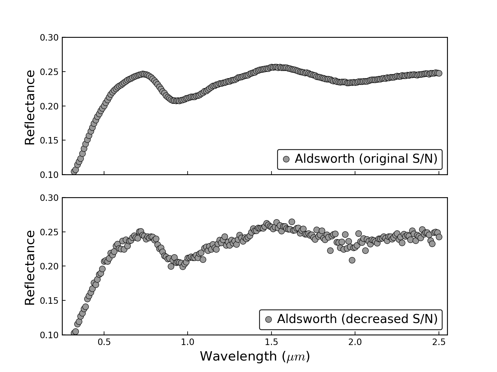
The first step in our analysis is to decrease the S/N of the ordinary chondrite spectra in order to reproduce the value measured for asteroid spectra. For this, we have chosen an S/N of 50, which is typically in the lower limit of NIR spectra obtained with the SpeX instrument on the NASA Infrared Telescope Facility (IRTF). The new degraded spectra were created with a Python code that makes use of the numpy.random.normal function (e.g., van der Walt et al., 2011). With this function it is possible to generate random samples from a normal (Gaussian) distribution, where the 1 used to create the random samples is calculated from the S/N that we choose, in this case 50 for the whole spectrum and about half of that value for the region between 1.8 and 2.1 m to simulate the effect of the telluric bands on the spectra. The S/N of the new spectra was then verified using the estimateSNR function of PyAstronomy111https://github.com/sczesla/PyAstronomy (Czesla et al., 2019). Figure 1 shows an example for the LL5 ordinary chondrite Aldsworth. The original spectrum (top panel) has an S/N of 600, while the S/N of the new spectrum has been decreased about 10 times (bottom panel).
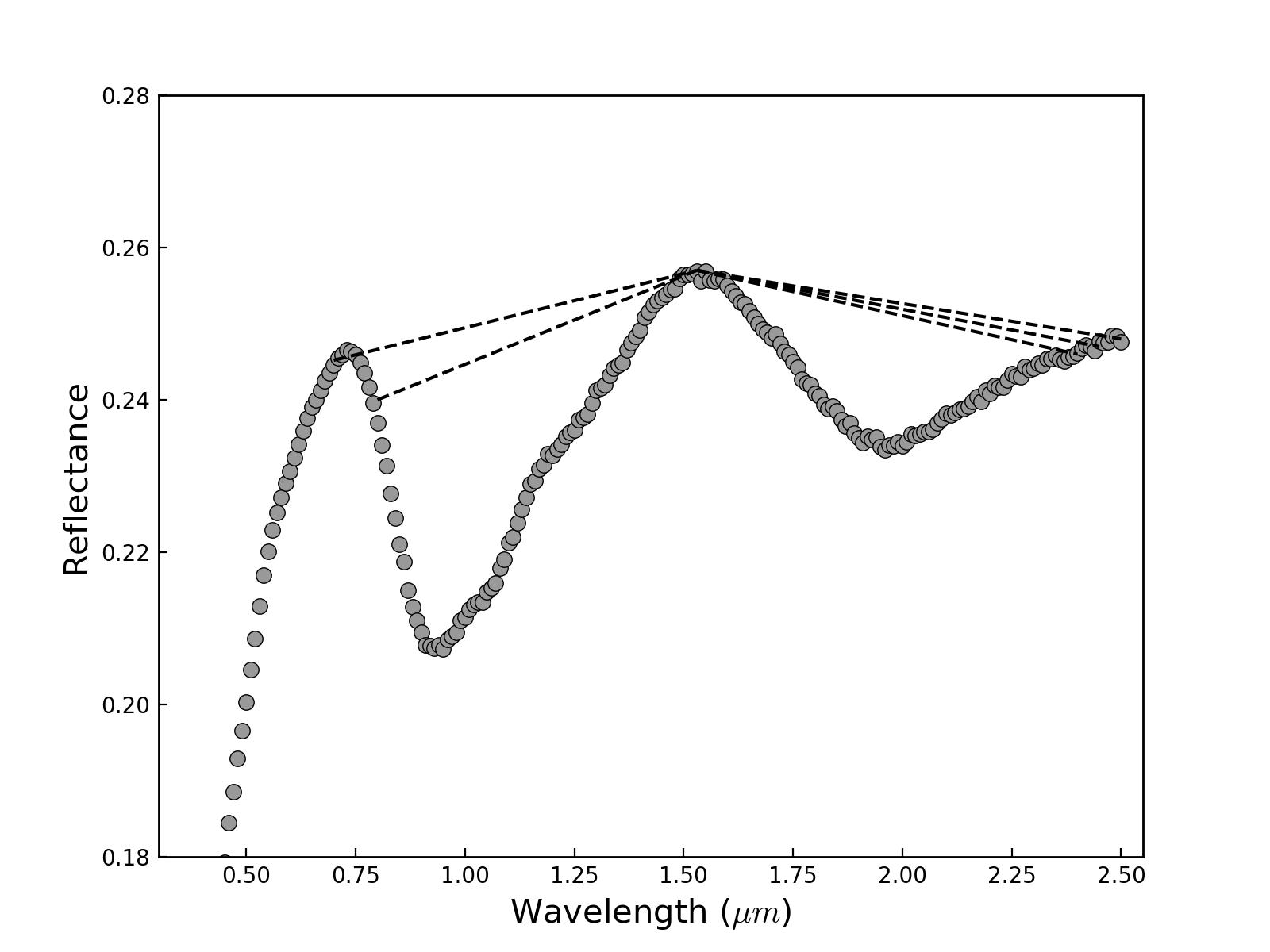
Spectral band parameters were measured using a Python code similar to the one used in Sanchez et al. (2015, 2017). Five different wavelength ranges were used in this study: 0.7-2.40 m, 0.7-2.45 m, 0.7-2.50 m, 0.8-2.40 m, and 0.8-2.45 m (Figure 2). The short wavelength edge of 0.7 m was chosen to include the local maximum at 0.74 m, that allow us to measure the continuum for Band I. The cutoff at 0.8 m was included to simulate the short wavelength edge of NIR spectra obtained with a 0.8 m dichroic filter, such as does obtained with the SpeX instrument on NASA IRTF prior to 2017. The cutoffs at 2.40 and 2.45 m were chosen to account for the decreased response of the detector for wavelengths beyond 2.4 m. The wavelength range of 0.7-2.50 m was included mostly to compare our results with those of Dunn et al. (2010a). Although Dunn et al. (2010a) used spectra in the range of 0.32-2.55 m, the effective wavelength range used to extract the band parameters was 0.7-2.50 m. The procedure used to measure the band parameters for the five wavelength ranges was different. For the three wavelength ranges encompassed between 0.7 and 2.50 m, reflectance maxima were determined by fitting third-order polynomials at 0.74 and 1.4 m, and a straight line from 2.20 to 2.40, 2.45, and 2.50 m. The linear continuum was then fitted from the reflectance maxima at 0.74 to the reflectance maxima at 1.4 m, and from 1.4 m to the three different wavelength ends. After dividing out the linear continuum, band centers were calculated by fitting a polynomial over the bottom third of Band I and bottom half of Band II. For the Band I center, 50 measurements were obtained by sampling slightly different wavelength ranges of data points. This was done for two consecutive polynomial orders ranging from second to fourth order. This is because we noticed that for some spectra higher polynomial orders yield a better fit. The final value is given by the average of the 100 measurements obtained for the two different polynomial orders, e.g., the average of a second and a third or, if higher polynomials were required to obtain a better fit, the average of a third and a fourth. The Band II center was calculated by taking the average value of a second and a third polynomial order in all cases, since the shape of the Band II is not as complex as the Band I, and in general shows more scattering due to an incomplete correction of the telluric bands. The BAR is calculated as the ratio of the area of Band II to that of Band I. Band areas are defined as the area between the linear continuum and the data curve, and are calculated using trapezoidal numerical integration. Like the Band centers, 100 measurements were done, but in this case, by slightly varying the position where the linear continuum was fitted, the average of these measurements was taken to obtain the final value. Errors associated with these parameters are given by the standard deviation of the mean. For the 0.8-2.40 and 0.8-2.45 m wavelength ranges, the procedure to measure the band parameters was very similar, the main differences being that the reflectance maximum at 0.8 m was determined by fitting a straight line from 0.8 to 0.86 m, and the Band I center was calculated by fitting a polynomial over the bottom half of the Band I, since the area of this band was now smaller than in the previous case.
4 Results
4.1 Olivine-pyroxene abundance ratio
Figure 3 shows the Band I center vs. BAR measured for the LL, L, and H ordinary chondrites for the five different wavelength ranges. The polygonal region corresponding to the S(IV) subgroup of Gaffey et al. (1993) is also indicated. Overall, we noticed that our Band I centers are shifted to shorter wavelengths compared to the values measured by Dunn et al. (2010a). For example, for the 0.7-2.5 m wavelength range (the same used by Dunn et al., 2010a), there is a difference of 0.02 m in the Band I center for the LL and L, and a difference of 0.01 m for the H chondrites. This difference is mostly the result of the polynomials used to determine the band centers. Dunn et al. (2010a) only used a second-order polynomial, whereas we used second- to fourth-order polynomials. Our results are consistent with the findings of Mitchell et al. (2020).
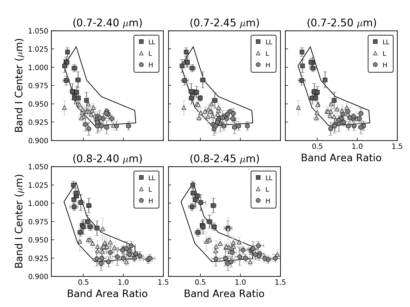
In the case of the BAR, for the three wavelength ranges encompassed between 0.7 and 2.50 m, values will shift to the left as the furthest data point moves from 2.50 to 2.40 m. The same happens for the two wavelength ranges encompassed between 0.8 and 2.45 m, however because the 1 m band was truncated at 0.8 m, BAR values are larger compared to those measured in the range of 0.7-2.50 m. As a result, some H chondrites are shifted to the right and now fall in the S(VI) subgroup (BAR 1.2-1.5) of Gaffey et al. (1993).
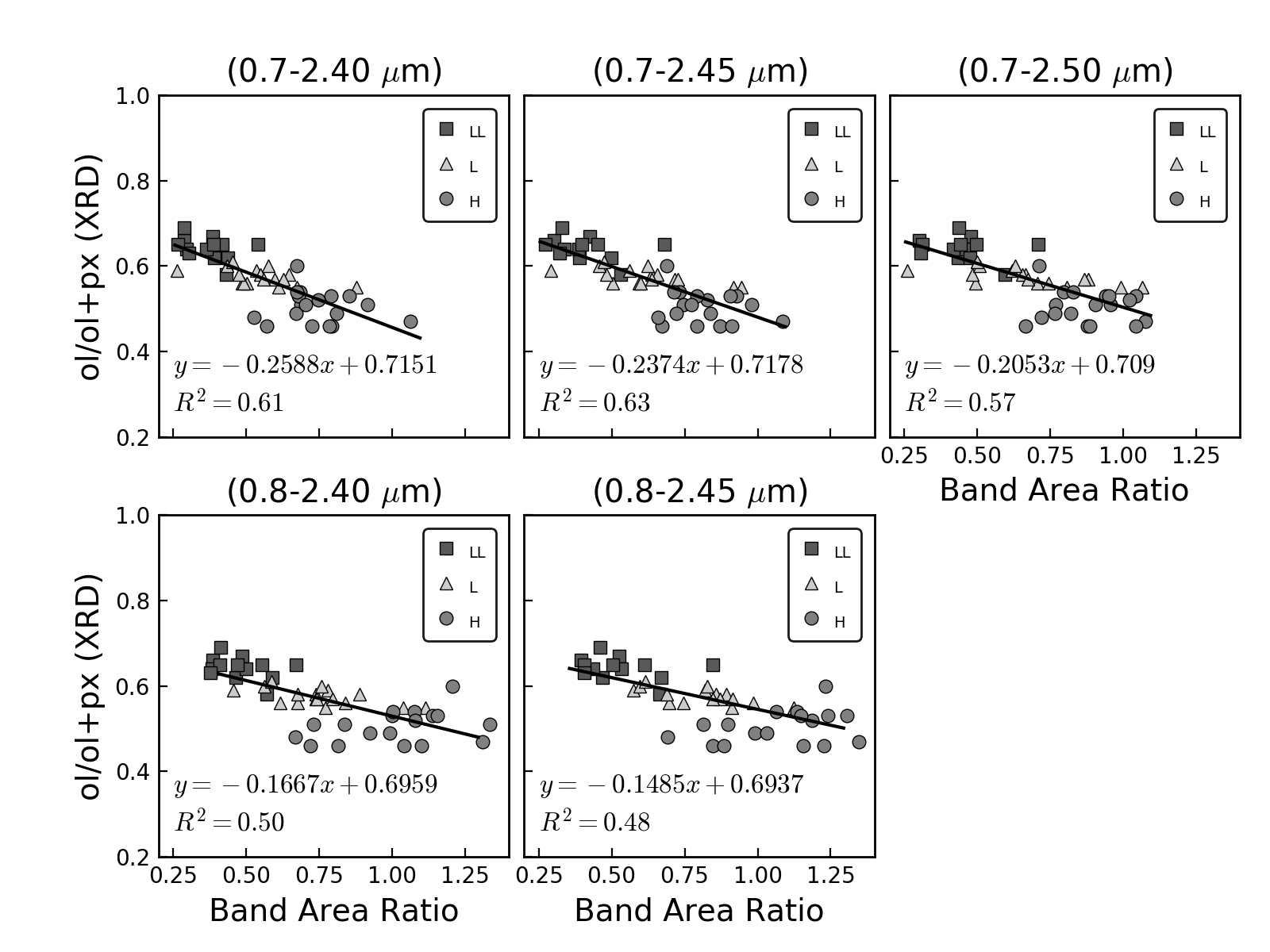
Following the same procedure used by Dunn et al. (2010a) we derived new equations for determining the olivine-pyroxene abundance ratio (ol/(ol+px)) using the BAR values and the XRD-measured modal abundances. Figure 4 shows the XRD-measured ol/(ol+px) ratio vs. BAR and the linear fits for the five different wavelength ranges. The new spectral calibrations are presented in Table 1. For the five equations, the root mean square error (rms) of the spectrally derived ol/(ol+px) ratios is 0.04. The rms is slightly higher than the uncertainty of 0.03 obtained by Dunn et al. (2010a) for the original equation. We found that the coefficient of determination (R2) varies from 0.48 (worse case corresponding to the 0.8-2.45 m range) to 0.63 (best case for the 0.7-2.45 m range).
4.2 Iron abundance in silicate minerals
Dunn et al. (2010a) found a strong correlation between the Band I center and the iron abundance in olivine (Fa) and pyroxene (Fs). Similarly to Dunn et al. (2010a), we found that this correlation can be described by a second-order polynomial fit (Figure 5).
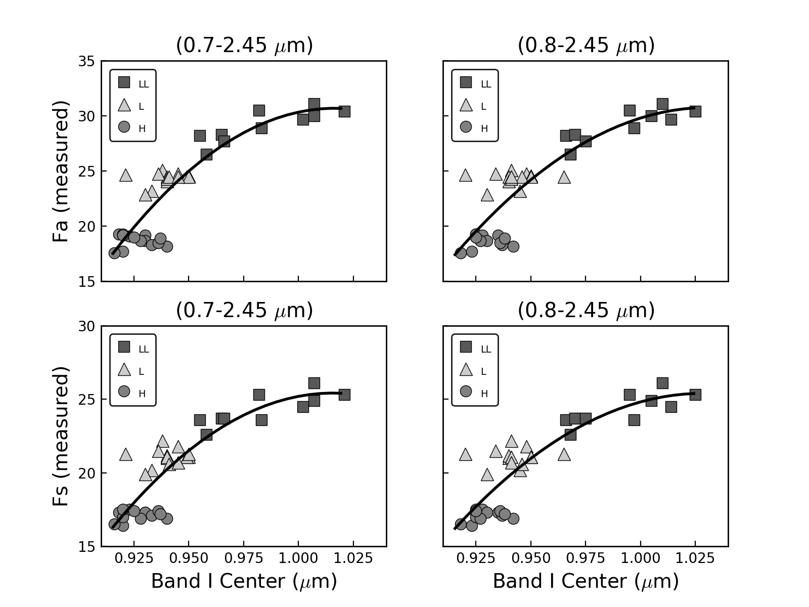
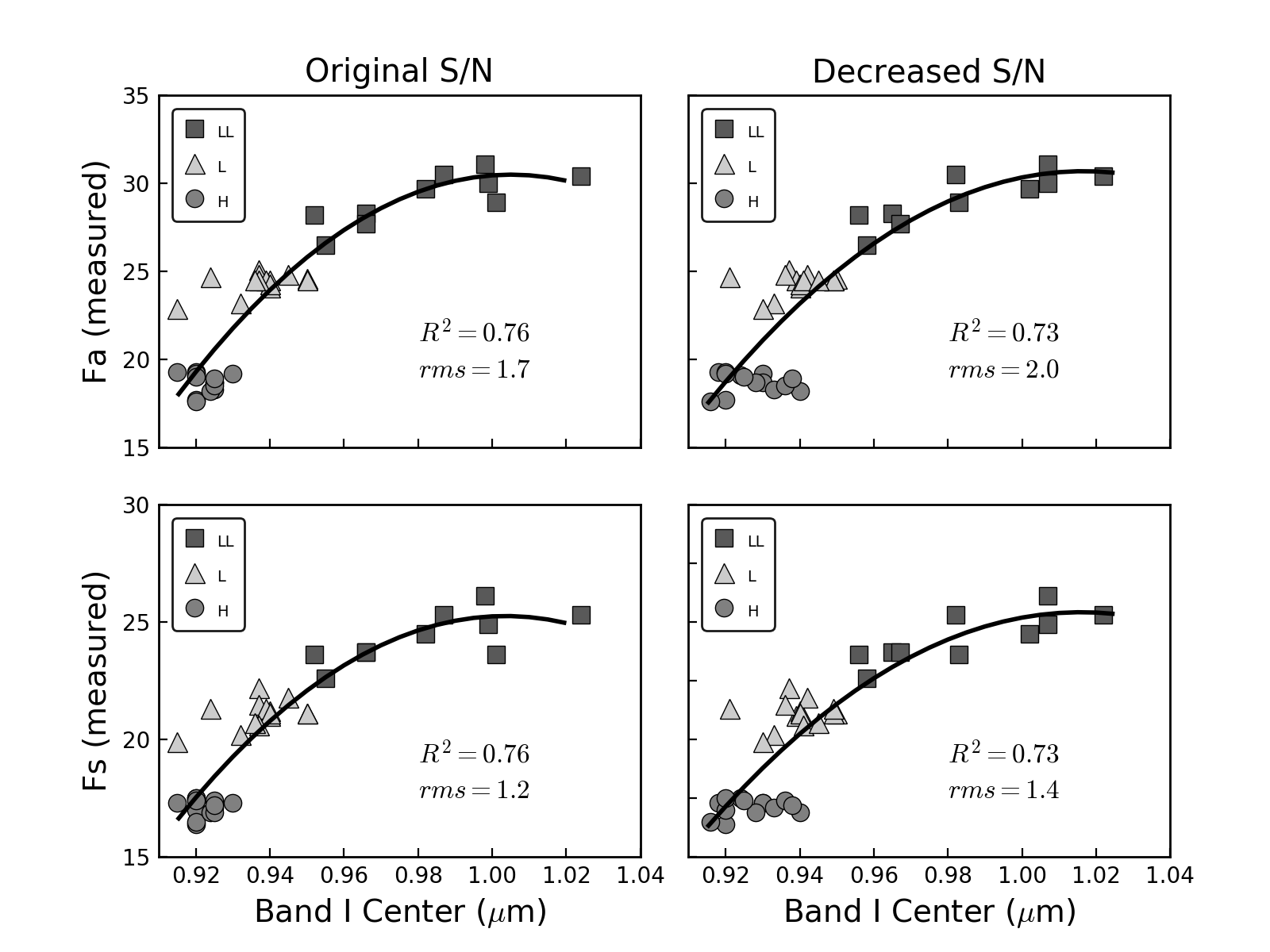
The Band I center is not affected by changes in the long wavelength end, thus the same equation can be used for the three wavelength ranges encompassed between 0.7 and 2.50 m. An example for the 0.7-2.45 m wavelength range is shown in Figure 5 (left panels). We observed some variations in the Band I center when the short wavelength edge was changed from 0.7 to 0.8 m. This is due to a difference in the spectral slope of the continuum that occurs when the reflectance maximum at the short wavelength edge is changed. Therefore, equations for the two wavelength ranges encompassed between 0.8 and 2.45 m were also derived (Figure 5, right panels). The new equations to determine the mol% of Fa and Fs are included in Table 1. The rms errors for Fa and Fs were found to be 2.0 and 1.4, respectively.
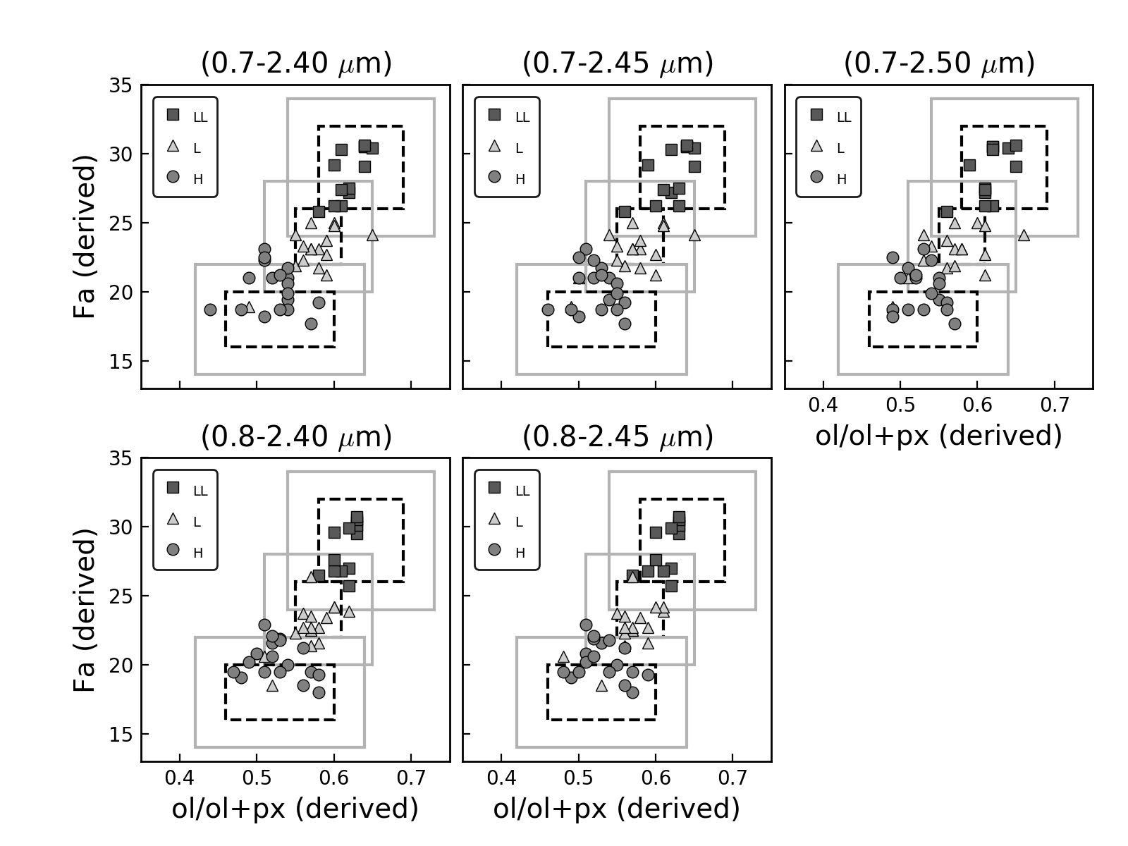
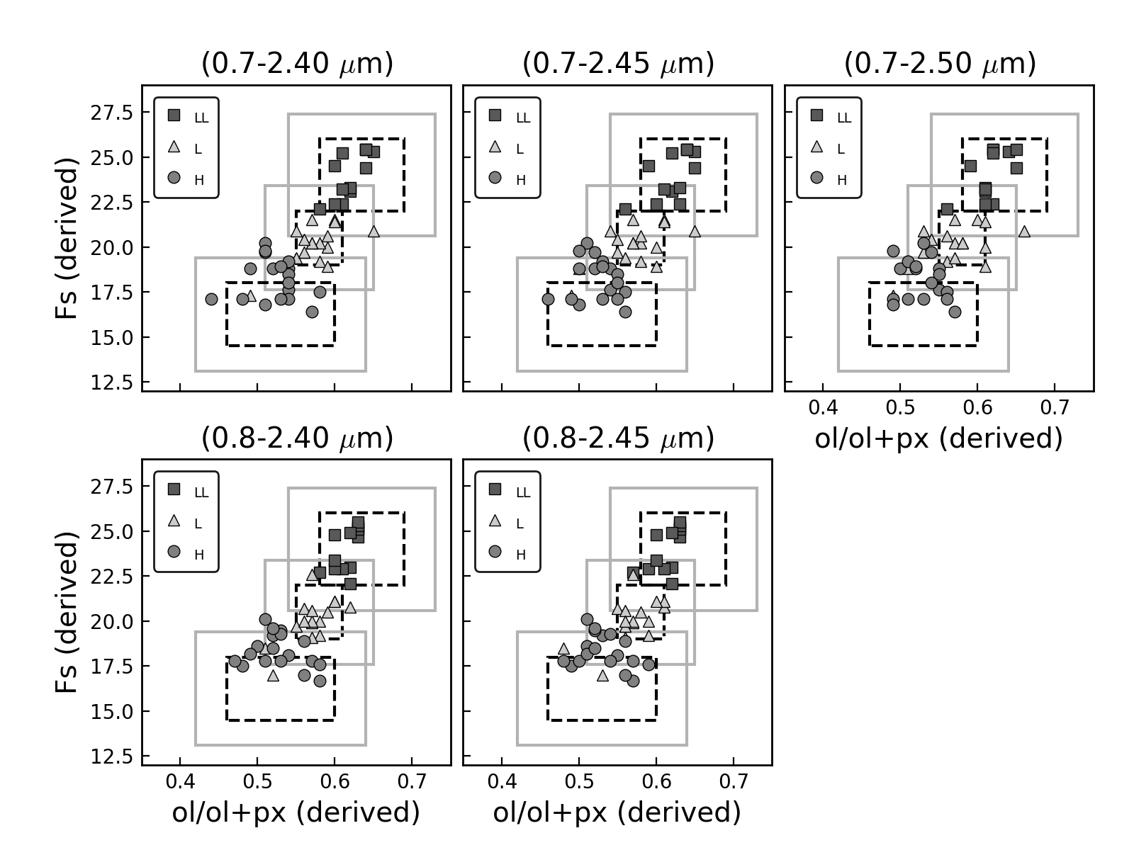
Thomas et al. (2014) discussed the limitations of using the quadratic equations of Dunn et al. (2010a) to determine the olivine and pyroxene chemistry. They noticed that the local maxima of the equations are within the range of the laboratory measured Fa and Fs values of the LL chondrites. As a result, the turnover in the equations will impose an artificial upper limit in the spectrally derived iron abundances of LL chondrites. Since we have also used quadratic equations, the same artificial limit is expected to occur, causing in some cases an underestimation in the iron abundances of asteroids with similar compositions. However, this will not affect the classification of objects into this ordinary chondrite subgroup. The spectrally derived ol/(ol+px) ratios and Fa and Fs values are combined in Figures 6 and 7 for the five different wavelength ranges. In these figures, which have been adapted from the original work of Dunn et al. (2010a), black dashed boxes represent the range of laboratory measured values for each ordinary chondrite subgroup (Dunn et al., 2010a), and gray solid boxes correspond to the uncertainties associated with the spectrally derived values in this work, i.e., 0.04 for the ol/(ol+px) ratio and 2.0 and 1.4, for Fa and Fs, respectively.
| Equation No. | Wavelength Range (m) | Spectral Calibration | R2 | rms |
|---|---|---|---|---|
| (1) | 0.7-2.50 | ol/(ol+px)=-0.2053xBAR+0.709 | 0.57 | 0.04 |
| (2) | 0.7-2.45 | ol/(ol+px)=-0.2374xBAR+0.7178 | 0.63 | 0.04 |
| (3) | 0.7-2.40 | ol/(ol+px)=-0.2588xBAR+0.7151 | 0.61 | 0.04 |
| (4) | 0.8-2.45 | ol/(ol+px)=-0.1485xBAR+0.6937 | 0.48 | 0.04 |
| (5) | 0.8-2.40 | ol/(ol+px)=-0.1667xBAR+0.6959 | 0.50 | 0.04 |
| (6) | 0.7-2.40,2.45,2.50 | Fa=-1283.4x(BIC2)+2609.5x(BIC)-1295.8 | 0.73 | 2.0 |
| (7) | 0.8-2.40,2.45 | Fa=-1002.5x(BIC2)+2066.5x(BIC)-1034.2 | 0.74 | 2.0 |
| (8) | 0.7-2.40,2.45,2.50 | Fs=-904.4x(BIC2)+1837.3x(BIC)-907.7 | 0.73 | 1.4 |
| (9) | 0.8-2.40,2.45 | Fs=-717.1x(BIC2)+1475.3x(BIC)-733.3 | 0.73 | 1.4 |
4.3 The effect of decreasing the S/N
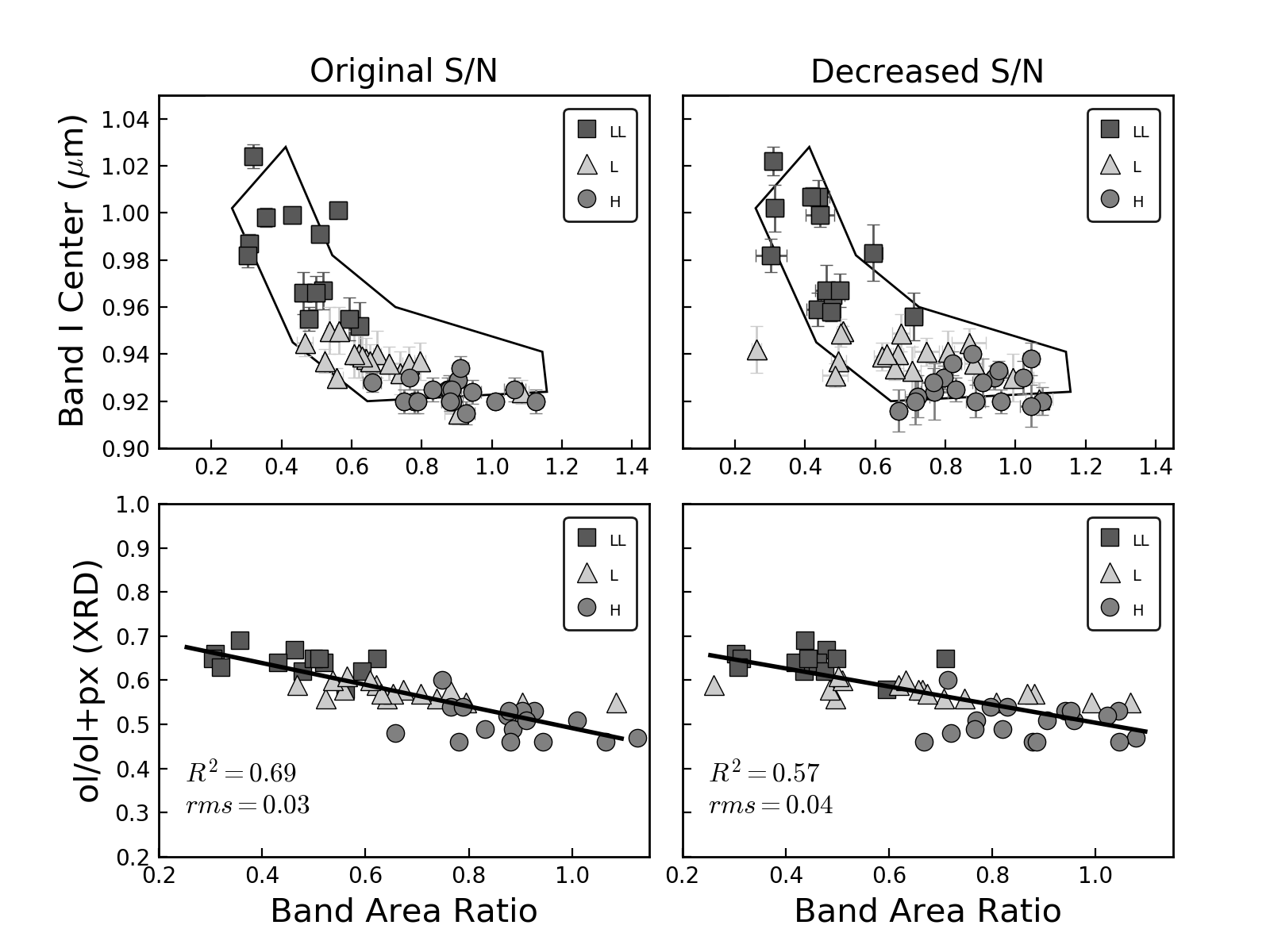
As explained earlier, the first step in our analysis was to decrease the S/N of the laboratory spectra in order to recreate the S/N observed among asteroid spectral data, and thus obtain more realistic results. We found that the major effect of doing this was an overall decrease in the R2, and an increase of the rms values of the new spectral calibrations. In other words, the lower R2 and higher rms are a consequence of a greater point-to-point scatter in the data resulting from spectra with a much lower S/N. This can be seen in Figure 8, where we compare the Band I center and BAR measured from the original spectra with those measured from the spectra with lower S/N (top panels) for the 0.7-2.50 m wavelength range. The XRD-measured ol/(ol+px) ratio vs. BAR are shown in the bottom panels. The R2 corresponding to the original data is higher than the value obtained from the noisy spectra and closer to the R2 (0.73) obtained by Dunn et al. (2010a).
The decrease in S/N was also found to produce a general shift of the Band I center to longer wavelengths, being more pronounced for the LL and H chondrites. Figure 9 shows measured Fa and Fs values as function of the Band I center for the original spectra (left), and the noisy spectra (right) for the 0.7-2.50 m range. This shift in Band I centers will make it harder to differentiate between L and H chondrites, which explains the tendency for the H chondrites to group in the upper part of their box (Figures 6 and 7), overlapping with some L chondrites. The difference in R2 and rms between the original and decreased S/N was found to be small for the five wavelength ranges.
4.4 The effect of changing the short wavelength edge
Lindsay et al. (2016) highlighted the importance of matching how Bands I and II are defined to the methods used to derive calibration equations. Using the same 48 ordinary chondrites used in this study, and the Dunn et al. (2010a) study, they examined how frequently a long wavelength edge, dubbed the “red edge,” of Band II set to 2.40 m and 2.45 m resulted in ol/(ol+px) values that were larger than the rms error from the meteorite calibration equations. When using a 2.40 m red edge compared with a 2.50 m red edge, they observed that changes in the BAR ratio resulted in ol/(ol+px) determinations outside of the rms error of the calibration equation for 41.67% of the ordinary chondrite meteorites overall. For each subgroup, the choice of the red edge was the largest source of error for 72.2% of the H chondrites, 29.4% of the L chondrites, and 15.4% of the LL chondrites.
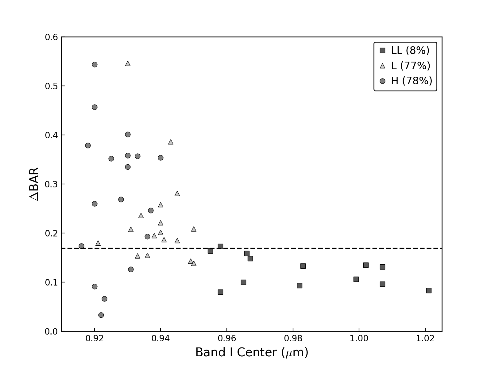
In order to investigate the extent to which changing the short wavelength edge (blue edge) is a problem, we have performed a similar analysis to the one employed by Lindsay et al. (2016) with the red edge. In our case, the difference lies in that we quantify the variation in BAR when the blue edge is changed from 0.7 to 0.8 m, while keeping the long wavelength end fixed at 2.45 m. The difference between the BAR values measured at the two different blue edges is given by the BAR, which is plotted as a function of the Band I center in Figure 10. Lindsay et al. (2016) defined a critical BAR in order to identify those cases where the error associated with the red edge choice was higher than the intrinsic calibration error associated with the equation to estimate the ol/(ol+px) ratio derived by Dunn et al. (2010a). We have defined a similar critical BAR for the blue edge, which can be calculated from the linear equations used to estimate the ol/(ol+px) ratio from the BAR (Equations (1)-(5) in Table 1). For this particular example, where we are keeping the long wavelength end fixed at 2.45 m, we use equation 2 of Table 1. The critical BAR is then calculated as BARcrit = 0.04/0.2374 = 0.1685, where 0.04 is the rms error, and 0.2374 is the coefficient in equation 2. The idea with this exercise is to identify those cases where the uncertainty associated with the blue edge choice (i.e., 0.7 or 0.8 m) is higher than the intrinsic calibration error in equation 2. The BARcrit is depicted in Figure 10 as a dashed line; meteorites that fall above this line have BARs greater than the error inherent in equation 2. We found that for LL chondrites the percentage of time that the 0.8 m blue edge is problematic is 8%, whereas for L and H chondrites is 77, and 78%, respectively. These results highlight the necessity to derive new equations to account for this problem.
4.5 Discussion
Reddy et al. (2014) verified the validity of the equations of Dunn et al. (2010a) comparing the spectrally derived olivine and pyroxene chemistry of near-Earth asteroid (25143) Itokawa with those measured from samples returned by the Hayabusa spacecraft. They found a difference of less than 1 mol% between the spectrally derived Fa and Fs values and the laboratory measurements. In this section we test if the new equations derived from spectra with a much lower S/N, using higher polynomial orders, and different wavelength ranges are still capable of producing similar results. For this, we measured the spectral band parameters from the NIR spectrum of Itokawa obtained by Binzel et al. (2001) with the IRTF. Band centers and the BAR were measured following the same procedure used with the ordinary chondrite spectra. A temperature correction was applied to the BAR in order to account for the difference between the room temperature at which the equations were derived and the lower surface temperature of the asteroid (e.g., Sanchez et al., 2012). Equations (1)-(5) (Table 1) were then used to calculate the ol/(ol+px) ratio for the five wavelength ranges. The Band I center was used with equations (6)-(9) to calculate the mol% of Fa and Fs. Spectral band parameters, Fs, Fa, and ol/(ol+px) values calculated for Itokawa are shown in Table 2.
| Wavelength Range (m) | Band I Center (m) | BAR | Temp. corrected BAR | Fa (mol%) | Fs (mol%) | ol/(ol+px) |
|---|---|---|---|---|---|---|
| 0.7-2.50 | 0.9780.005 | 0.400.05 | 0.380.05 | 28.72.0 | 24.11.4 | 0.630.04 |
| 0.7-2.45 | 0.9780.005 | 0.380.05 | 0.360.05 | 28.72.0 | 24.11.4 | 0.630.04 |
| 0.7-2.40 | 0.9780.005 | 0.350.05 | 0.320.05 | 28.72.0 | 24.11.4 | 0.630.04 |
| 0.8-2.45 | 0.9920.005 | 0.550.05 | 0.530.05 | 29.22.0 | 24.51.4 | 0.620.04 |
| 0.8-2.40 | 0.9920.005 | 0.510.05 | 0.490.05 | 29.22.0 | 24.51.4 | 0.610.04 |
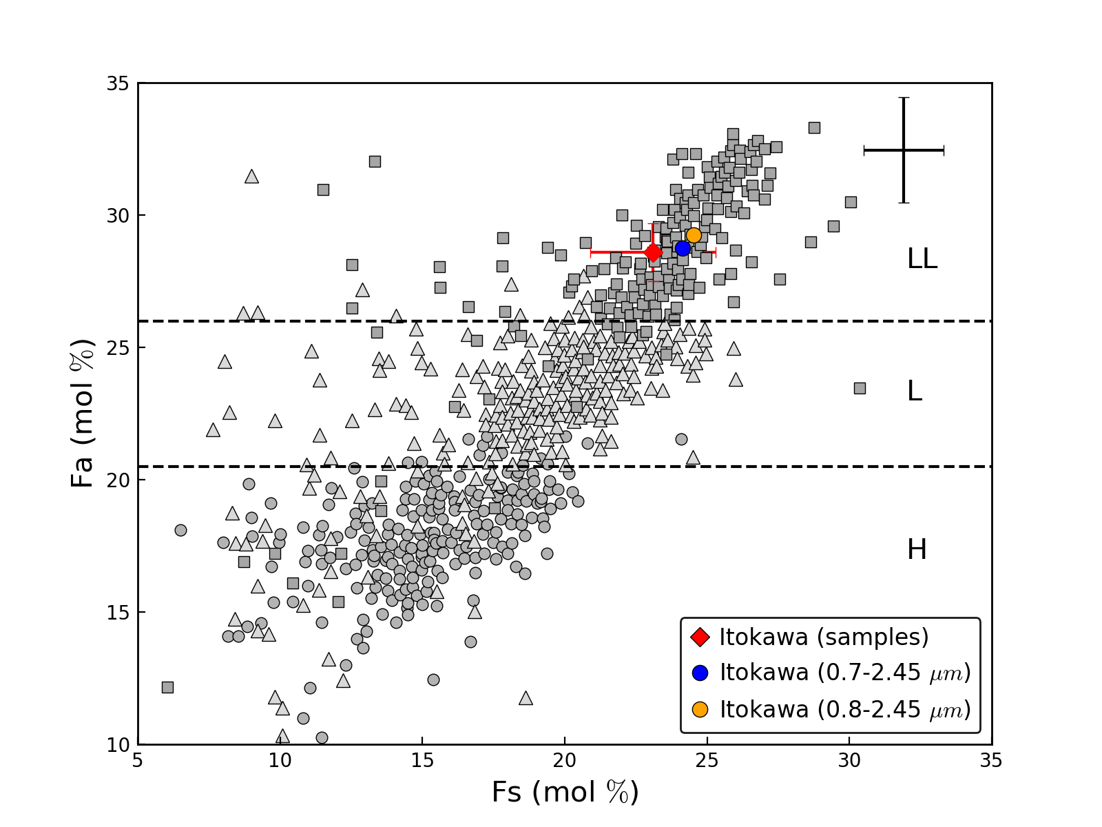
For the three wavelength ranges encompassed between 0.7 and 2.50 m, the olivine and pyroxene chemistries of Itokawa were found to be Fa28.7±2.0 and Fs24.1±1.4. Higher values were obtained for the wavelengths in the range of 0.8-2.45 m, Fa29.2±2.0 and Fs24.5±1.4, but in both cases within the uncertainties. These results are very close to the mean values measured from the samples (Fa28.6±1.1 and Fs23.1±2.2) by Nakamura et al. (2011). Spectrally derived olivine and pyroxene chemistries for Itokawa and laboratory measurements are shown in Figure 11.
No significant variation was observed for the calculated ol/(ol+px) ratios for the five wavelength ranges; the lowest value was found to be 0.610.04 (0.8-2.40 m range) and the highest was 0.630.04 for the three wavelength ranges encompassed between 0.7 and 2.50 m. These results are similar to the one derived by Dunn et al. (2013), who obtained an ol/(ol+px) ratio of 0.600.03 for Itokawa using the original equation. We noticed, however, that our spectrally derived values are lower than the ol/(ol+px) ratio measured from the samples by Tsuchiyama et al. (2014) (0.760.10). This difference could be attributed to the limited amount of sample returned from Itokawa. Contrary to the disk-integrated spectrum, which represents a large fraction of the object, modal abundances measured from a few regolith particles of Itokawa might not be representatives of the entire asteroid. In addition, it is also possible that among the 48 ordinary chondrites used in this study, there were not enough olivine-rich LL chondrites. The highest XRD ol/(ol+px) ratio measured for the ordinary chondrites (0.690.03) corresponds to the LL6 chondrite Karatu (Dunn et al., 2010c). Thus, adding more LL chondrites with higher ol/(ol+px) ratios would increase the slope of the linear regressions in Figure 4, increasing with this the spectrally derived ol/(ol+px) ratios of asteroids with a similar composition. Future studies could benefit from adding more samples, and in particular, more olivine-rich LL chondrites.
The example presented in this section demonstrates that the equations derived for the different wavelength ranges yield similar results. The user has to decide which equations are the most appropriate for a given data set. For example, prior to 2017 it was a common practice to use a 0.8 m dichroic filter with the SpeX instrument on the IRTF, as a result, hundreds of asteroid spectra were truncated at this wavelength (e.g., the MITHNEOS data set; (Binzel et al., 2019)). In a case like this, the equations derived for the 0.8-2.45 m wavelength range have to be applied. On the contrary, if the spectra include the local maximum at 0.74 m, then the equations derived for the 0.7-2.50 m wavelength range should be used, since they seem to yield slightly more accurate results as seen in Figure 11. As for the long wavelength end of the spectrum, a visual inspection could help to determine which cutoff (2.40, 2.45, or 2.5 m) to apply depending on the scattering of the data at these wavelengths.
4.6 Summary
In this study we have complemented the original work of Dunn et al. (2010a) by deriving new spectral calibrations that can be used to determine the mineral composition and abundance of ordinary chondrite-like S-type asteroids, i.e., objects that fall in the S(IV) compositional subgroup of Gaffey et al. (1993). Our study, which makes use of the same sample consisting of 48 ordinary chondrites, has two major differences with respect to the work of Dunn et al. (2010a). The first difference is that we have decreased the S/N of the laboratory spectra from 600 to 50, in order to recreate the S/N typically observed among asteroid spectra. This step allowed us to obtain more realistic results in terms of the uncertainties associated with the new spectral calibrations. The second difference is that the new spectral calibrations were derived for five different wavelength ranges, allowing us to extend the work of Dunn et al. (2010a), so the composition of the asteroids can be estimated from incomplete data.
From our analysis we found that Band I centers are shifted to shorter wavelengths compared to the values measured by Dunn et al. (2010a). The shift in Band I center arises when the polynomial order used to calculate this parameter is higher than the second-order used by Dunn et al. (2010a). Therefore, the new spectral calibrations are more suitable if higher polynomial orders are needed to obtain a better fit of the absorption band. If a second-order polynomial is enough, then the original equations of Dunn et al. (2010a) should be used. Ultimately, if the procedure used to measure the band parameters is too different from the one employed in the present study and in Dunn et al. (2010a), new equations should be derived using that procedure.
As expected, the decrease in the S/N of the laboratory spectra caused a greater point-to-point scatter in the data, resulting in an overall decrease in the R2, and an increase of the rms values of the new spectral calibrations. The decrease in S/N was also found to produce a shift of the Band I center to longer wavelengths, producing more overlap between L and H chondrites.
We found that changing the blue edge of the spectra from 0.7 to 0.8 m will produce variations in the BAR, which for most L and H chondrites are higher than the intrinsic calibration error. These results highlight the importance of deriving new spectral calibrations for different wavelength ranges.
We tested the new spectral calibrations using the band parameters measured from the NIR spectrum of asteroid Itokawa, and comparing the results with laboratory measurements of the returned samples. We found that the spectrally derived olivine and pyroxene chemistry are in excellent agreement with the mean values measured from the samples. The derived mineral abundance, however, was found to be lower than the samples. This discrepancy could be related to the limited amount of regolith particles returned from Itokawa, which might not be representatives of the entire asteroid.
References
- Adams (1974) Adams, J. B. 1974, J. Geophys. Res., 79, 4829
- Binzel et al. (2001) Binzel, R. P., Rivkin, A. S., Bus, S. J., et al. 2001, Meteoritics and Planetary Science, 36, 1167
- Binzel et al. (2019) Binzel, R. P., DeMeo, F. E., Turtelboom, E. V., et al. 2019, Icarus, 324, 41
- Burbine et al. (2003) Burbine, T. H., McCoy, T. J., Jaresowich, E., et al. 2003, Antarctic Meteorite Research, 16, 185
- Burbine et al. (2009) Burbine, T. H., Buchanan, P. C., Dolkar, T., & Binzel, R. P. 2009, Meteoritics and Planetary Science, 44, 1331
- Burbine et al. (2018) Burbine, T. H., Buchanan, P. C., Klima, R. L., et al. 2018, Journal of Geophysical Research (Planets), 123, 1791
- Burns et al. (1972) Burns, R. G., Huggins, F. E., & Abu-Eid, R. M. 1972, Moon, 4, 93
- Bus, & Binzel (2002) Bus, S. J., & Binzel, R. P. 2002, Icarus, 158, 106
- Cloutis et al. (1986) Cloutis, E. A., Gaffey, M. J., Jackowski, T. L., & Reed, K. L. 1986, J. Geophys. Res., 91, 11641
- Czesla et al. (2019) Czesla, S., Schröter, S., Schneider, C. P., et al. 2019, PyA: Python astronomy-related packages, ascl:1906.010
- Dunn et al. (2010a) Dunn, T. L., McCoy, T. J., Sunshine, J. M., et al. 2010a, Icarus, 208, 789
- Dunn et al. (2010b) Dunn, T. L., Cressey, G., McSween, H. Y. _jr ., et al. 2010b, Meteoritics and Planetary Science, 45, 123
- Dunn et al. (2010c) Dunn, T. L., McSween, H. Y. _jr ., McCoy, T. J., et al. 2010c, Meteoritics and Planetary Science, 45, 135
- Dunn et al. (2013) Dunn, T. L., Burbine, T. H., Bottke, W. F., & Clark, J. P. 2013, Icarus, 222, 273
- Gaffey et al. (1993) Gaffey, M. J., Burbine, T. H., Piatek, J. L., et al. 1993, Icarus, 106, 573
- Gaffey et al. (2002) Gaffey, M. J., Cloutis, E. A., Kelley, M. S., & Reed, K. L. 2002, Asteroids III, 183
- Lindsay et al. (2016) Lindsay, S. S., Dunn, T. L., Emery, J. P., et al. 2016, Meteoritics and Planetary Science, 51, 806
- Lucas et al. (2019) Lucas, M. P., Emery, J. P., Hiroi, T., et al. 2019, Meteoritics and Planetary Science, 54, 157
- Mitchell et al. (2020) Mitchell, A., Reddy, V., Sharkey, Benjamin., et al. 2020, Icarus, 336, 113426
- Nakamura et al. (2011) Nakamura, T., Noguchi, T., Tanaka, M., et al. 2011, Science, 333, 1113
- Reddy et al. (2014) Reddy, V., Sanchez, J. A., Bottke, W. F., et al. 2014, Icarus, 237, 116
- Sanchez et al. (2012) Sanchez, J. A., Reddy, V., Nathues, A., et al. 2012, Icarus, 220, 36
- Sanchez et al. (2014) Sanchez, J. A., Reddy, V., Kelley, M. S., et al. 2014, Icarus, 228, 288
- Sanchez et al. (2015) Sanchez, J. A., Reddy, V., Dykhuis, M., et al. 2015, ApJ, 808, 93
- Sanchez et al. (2017) Sanchez, J. A., Reddy, V., Shepard, M. K., et al. 2017, AJ, 153, 29
- Thomas et al. (2014) Thomas, C. A., Emery, J. P., Trilling, D. E., et al. 2014, Icarus, 228, 217
- Tsuchiyama et al. (2014) Tsuchiyama, A., Uesugi, M., Uesugi, K., et al. 2014, Meteoritics and Planetary Science, 49, 172
- van der Walt et al. (2011) van der Walt, S., Colbert, S. C., & Varoquaux, G. 2011, Computing in Science and Engineering, 13, 22
- Xu et al. (1995) Xu, S., Binzel, R. P., Burbine, T. H., et al. 1995, Icarus, 115, 1