∎
e1e-mail: sunil@unizwa.edu.om \thankstexte2e-mail: kumar@gmail.com \thankstexte3e-mail: saibal@associates.iucaa.in \thankstexte4e-mail: d.deb32@gmail.com
A new model for spherically symmetric charged compact stars of embedding class one
Abstract
In the present study we search for a new stellar model with spherically symmetric matter and charged distribution under general relativistic framework. The model represents a compact star of embedding class one. The solutions obtain here are general in their nature having the following two features: firstly, the metric becomes flat and also the expressions for the pressure, energy density and electric charge become zero in all the cases if we consider the constant , which shows that our solutions represent the so-called ‘electromagnetic mass model’ Lorentz1904 , and secondly, the metric function , for the limit tends to infinity, converts to , which is the same as considered by Maurya et al. Maurya2015a . We have investigated several physical aspects of the model and find that all the features are acceptable within the demand of the contemporary theoretical studies and observational evidences.
Keywords:
general relativity, embedding class one, perfect fluid, electromagnetic field1 Introduction
It is well known that the , which is dimensional manifold, can always be embedded in dimensional Pseudo-Euclidean space. In essence is the minimum extra dimensions of pseudo-Euclidean space which is needed for the embedding class of . The embedding class turns out to be 6 as the relativistic spacetime is 4 dimensional. The class of general spherical and plane symmetric spacetime are 2 and 3 respectively. The Friedman-Robertson-Lemaître spacetime Friedmann1922 ; Robertson1933 ; Lemaitre1933 is of class 1, but the Schwarzschild exterior and interior solutions are of class 2 and class 1 respectively. Moreover the Kerr metric is of class 5 Kuzeev1980 . However, in the present investigation our discussion is limited to the static spherically symmetric metric in curvature coordinates which is embedable in pseudo Euclidean space and hence is of embedding class one metric.
It is well known that the aforesaid metric is only compatible with two perfect fluid distributions: the first one is the Schwarzschild interior solution Schwarzschild1916 with de Sitter’s and Einstein’s universe as its particular cases, and the second one is the Kohler-Chao solution Kohlar1965 . It is worth to point out that the former one is conformally flat while the latter one is non-conformally flat.
Presently we would like to utilize the embedding class one metric to construct electromagnetic mass models by obtaining charged perfect fluid distributions. Normally when charge can be made zero in a charge fluid distribution, then the subsequent distribution is neutral counterpart of the charged distribution. For example, if we get Schwarzschild’s interior metric after the removal of charge in a charged fluid, then that is called charged analogue of the Schwarzschild interior solution Schwarzschild1916 . On the other hand, if the metric of charged fluid turns out to be flat and also all the physical parameters like pressure, density vanish, the corresponding charged fluid distribution is said to form an electromagnetic mass model, i.e. the entire mass is made up of charge only.
This type of electromagnetic mass model (EMMM) with vanishing charge density was first proposed by Lorentz Lorentz1904 and later on by several other scientists Wheeler1962 ; Feynman1964 ; Florides1974 ; Tiwari1984 ; Gautreau1985 ; Gron1985 ; Gron1986 ; Cooperstock1989 ; Tiwari1991a ; Tiwari1991b ; Tiwari1991c ; Ray1993 ; Ray1997 ; Wilzchek1999 ; Ray2002a ; Ray2002b ; Ray2004a ; Ray2004b ; Ray2006 ; Ray2007b . Unfortunately, in all these electromagnetic mass models the fluid has negative pressure (tension). However, it is true for gaseous spheres though at the boundary the vanishing of the density is not necessary for junction conditions. A model with such a special type of density have been proposed both for the uncharged as well as charged cases Mehra1980 ; Kuchowicz1968 . Another idea about the electromagnetic origin of the electron mass maintains that, due to vacuum polarization, its interior has the equation of state of the kind
| (1) |
where and represents the density and the pressure respectively. This leads to repulsive pressure and easier junction conditions Florides1974 ; Krori1975 ; Gron1986 ; Cooperstock1989 . It can also be combined with a Weyl-type character of the field Ray1993 . The experimental evidence that the electron’s diameter is not larger than cm leads to the conclusion that the classical model of electron must have a region of negative density Ray1997 .
In this paper we have considered the metric for . The choice of constraint on is due to the following reasons: (i) for , there is no meaning of here in the present context as the spacetime via becomes flat, (ii) for , this reduces to the same as the Kohlar-Chao solution Kohlar1965 , and (iii) for the term in the expression of takes the place in the denominator. We have calculated the data for to and wanted to see what would happen in the result for very high value of . So, one can look in to the Table 2 that if be large enough i.e. , 1000 and even more then becomes approximately a constant, say . This means if we take limit tends to infinity then the metric will convert to the following form , which is the same as metric considered for the solution of EMMM Maurya2015a .
In the present work we shall try to form a model for the charged fluid of class one by assuming specific metric potential(s) of the class one metric such that they do not form sub set of the metric potentials of the Kohler-Chao metric Kohlar1965 and the Schwarzschild interior metric (considering de Sitter and Einstein universe) Schwarzschild1916 . Now, if the charge can be made zero in the charged fluid so obtained, the describing metric will turn out to be flat by virtue of the class one structure of the metric.
Outline of the present investigation is as follows: in Sect. 2 the field equations and some specific results are provided under the Einstein-Maxwell spacetime whereas we obtain a new class of solutions in Sect. 3. The matching conditions are discussed in Sect. 4 and physical properties of the model are explored in Sect. 5. We pass some comments in Sect. 6.
2 The field equations and the results
2.1 The Einstein-Maxwell spacetime
Let us consider the static spherically symmetric metric in the form
| (2) |
The Einstein-Maxwell field equations can be given as
| (3) |
where in relativistic geometric unit and is the Einstein constant. The matter in the star is expected to be locally perfect fluid. However and are the energy-momentum tensor of fluid distribution and electromagnetic field respectively and that can be defined as
| (4) |
| (5) |
where is the energy density, is the pressure and is the four-velocity defined as .
2.2 The embedding class one spacetime
The metric (2) may represent spacetime of embedding class one, if it satisfies the given condition of Karmarkar Karmarkar
| (6) |
where Pandey1982 .
The above condition with reference to (2) yields the following differential equation
| (7) |
The solution of differential Eq. (7) can be furnished as
| (8) |
| (9) |
and
| (10) |
where is an arbitrary non-zero integration constant.
Using the spherically symmetric metric (2) and Eq. (8), the Einstein-Maxwell field equations can be written as the following set of equations Maurya2015a :
| (11) |
| (12) |
| (13) |
where the differential with respect to is denoted by prime.
3 A new class of solutions
To determine the expression for the electric charge, we use the pressure isotropy condition. Therefore, from Eqs. (11) and (12), we get
| (14) |
As a consequence of the above Eq. (14) we conclude that if charge vanishes in a charged fluid of embedding class one then the Schwarzschild interior solution Schwarzschild1916 (or special cases like de Sitter universe or the Einstein universe) or the Kohler-Chao solution Kohlar1965 will be only survived neutral counterpart unless either the survived spacetime metric is flat or the charge cannot be zero. Obviously, in the absence of charge either of two factors on the right hand side of (14) has to be zero. It can be verified that the vanishing of the first factor of (14) gives rise to the Kohlar-Chao solution. However, the vanishing of second factor ultimately provides the Schwarzschild interior solution.
Let us consider that is the mass function for electrically charged fluid sphere and can be given as
| (15) |
By plugging Eq. (8) and Eq. (14) into Eq. (15), eventually we get
| (16) |
We observe that the expressions for the pressure (), density (), electric charge () and mass () are dependent on metric function . As a consequence we consider the metric function to find the spherically symmetric charged fluid solutions in the following form
| (17) |
where is a positive number and is a constant such that and .
The above form of the metric potential represents the same as considered by Lake Lake2003 in his Eq. (9) for and . Therefore, the explanations on Eq. (17) are mostly the same as in the Ref. Lake2003 . The function is monotone increasing with a regular minimum at . If we look at the mass function in Eq. (16), then it is clear that by using this source function of Eq. (17), the mass function can easily be evaluated exactly for any . Thus, the metric function will generate a ‘class’ of solutions having the physical properties which are expected to be quite distinct for each value of . It is noted that previously the solutions for either Lake1998 or Maurya2011 solutions were known. With , constitute half of all the previously known physically interesting solutions in curvature coordinates Lake1998 whereas for solutions are acceptable on physical grounds and even exhibit a monotonically decreasing subluminal adiabatic sound speed Maurya2011 . It will be also interesting to note that the above form of is quite different from the function of Schwarzschild or Kohlar-Chao as one can get a hint from Eq. (14). Thus, in the present study we expect that each source function which is a monotone increasing function with a regular minima at necessarily provides, via the mass function in Eq. (16), a static spherically symmetric perfect fluid solution of Einstein’s equations which is regular at .
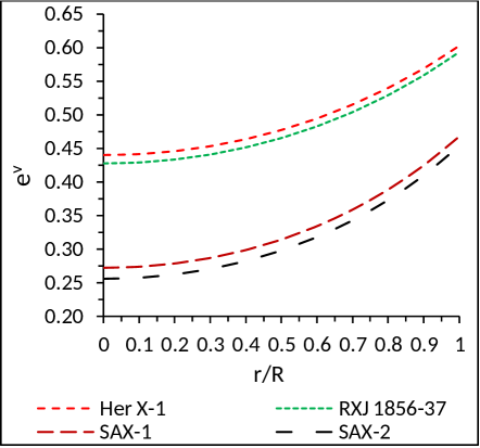
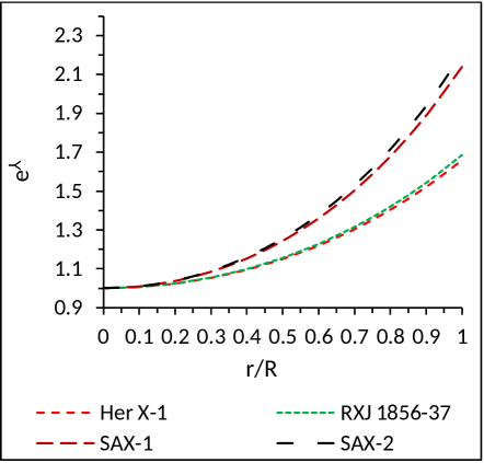
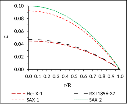
On the other hand, the metric potential can be obtained from Eq. (8) as
| (18) |
where and , are positive constants. In Fig. 1 the behaviour of and are shown.
The expressions of the electromagnetic mass and the electric charge are then given by
| (19) |
| (20) |
where , and .
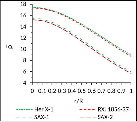
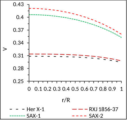
Similarly, the expression for the pressure and the energy density are given by (Fig. 2)
| (21) |
| (22) |
where , .
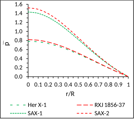
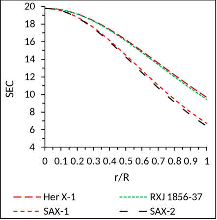
We suppose that the pressure of the charged fluid sphere is related with the energy density by a parameter as, , which is given by (Fig. 3)
| (23) |
We note from Fig. (3) that the ratio is less than 1 throughout inside the star. This obviously implies that the densities are dominating over the pressures everywhere inside the star and the underlying fluid distribution is non-exotic in nature Rahaman2010 .
The expressions for the pressure gradients (by taking ) are given by
| (24) |
| (25) |
where
| (26) |
| (27) |
| (28) |
| (29) |
| (30) |
| (31) |
4 Matching condition
For any physically acceptable charged solution, the following boundary conditions must be satisfied:
(i) The interior of metric (1) for the charged fluid distribution join smoothly with the exterior of Reissner-Nordström metric
| (32) |
at the surface of charged compact stars, whose mass is same as at .
(ii) The pressure must be finite and positive at the centre and it must be zero at the surface of the charged fluid sphere Misner .
By matching the first and second fundamental forms, the interior of the metric (2) and the exterior of the metric (32) at the boundary (the Darmois-Israel condition), we can find the constants , and . These are therefore can be obtained as follows:
| (33) |
| (34) |
| (35) |
where , .
However, the value of constant can be determined by assuming density at the surface of the star i.e. at , so that we get
| (36) |
where .
Also the value of constant can be determined by using the relation as
| (37) |
| Compact star | ||||
|---|---|---|---|---|
| candidates | () | |||
| Her. X-1 | 5.8164 | 0.4403 | 5.4406 | |
| RXJ 1856-37 | 5.7794 | 0.4274 | 4.2877 | |
| SAX J1808.4-3658(SS1) | 5.1682 | 0.2725 | 4.8944 | |
| SAX J1808.4-3658(SS2) | 5.0772 | 0.2560 | 3.8540 |
5 Physical features of the charged compact star models
Let us look at the results so far we have obtained in the previous section. A close observation of the results immediately reveals the following two distinct features:
(i) The metric (2) becomes flat and also the expressions for all the physical parameters, viz. pressure, energy density, electric charge etc., become zero in all the cases if we take . This feature shows that our solutions represent the so-called ‘electromagnetic mass model’ Lorentz1904 .
(ii) In this work we have taken the metric function , with and have calculated the data of the stellar models for to . We come across a very interesting result that when we increase the value of at very large, say more than 100, then the product becomes approximately a constant (see Table 2). So for the limit tends to infinity, the present metric potential in Eq. (17) will convert to the following form:
which is the same as considered by Maurya et al. Maurya2015a . However, the nature of the present models, at very large value of i.e. at infinity, can be seen in Ref. Maurya2015a .
Let us now, besides the above two general features, try to explore some other physical behaviour of our models.
5.1 Regularity condition
(i) Potentials at the centre : From Eqs. (17) and (18), we observe that the metric potentials at the centre becomes and . This implies that metric potentials are singularity free and positive at the centre. However, both are monotonically increasing function (Fig. 1).
(ii) Pressure at the centre : From Eq. (21), one can obtain , where and are positive numbers. Hence, the pressure should be positive at the centre and this implies that .
(iii) Density at the centre : From Eq. (22), we get the central density which must be positive at the centre. Since is positive so is also positive due to positivity of . We know that , where , , all are positive. This implies that is also a positive quantity.
5.2 Casuality and Well behaved condition
The speed of sound must be less than the speed of light i.e. . However, for well behaved nature of charged solution, Canuto Canuto argued that the speed of sound should monotonically decrease outwards for the equation of state with an ultra-high distribution of matter. Form Fig. 4, one can observe that the speed of sound is monotonically decreasing outwards. This implies that our model for charged fluid is well behaved.
It can also be observed from Fig. 4 that the velocity of sound starts decreasing from and this clearly indicates that the solution is physically valid for the values from onwards. However, one thing is then important to know what will happen for increasing of towards very large value. It seems possible to get a reasonable model even when tends to infinity. This is because the product of becomes approximately constant for large value of . So if we take tends to infinity the metric reduces to the case of Ref. Maurya2015a as discussed earlier in the introductory part of this Sect. 5.
5.3 Energy Conditions
For physically valid charged fluid
sphere, the null energy condition (NEC), strong energy condition
(SEC) and weak energy condition (WEC), all must satisfy
simultaneously at all the interior points of the star. Therefore,
in our model the following inequalities should hold good:
NEC: , WEC: , SEC: .
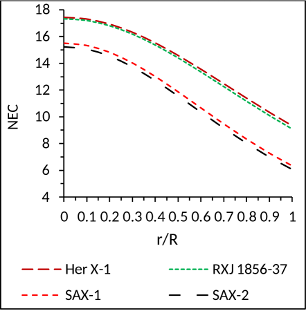
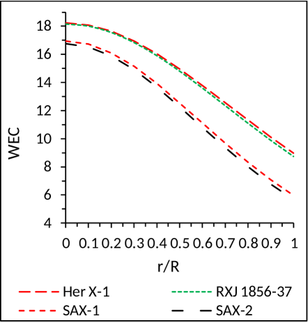
In Fig. 5 we have shown the energy conditions which are as par physical requirement.
5.4 Generalized TOV equation
The generalized Tolman-Oppenheimer-Volkoff (TOV) equation Tolman1939 ; Oppenheimer1939
| (38) |
where is the effective gravitational mass given by
| (39) |
Eq. (38) describes the equilibrium condition for a charged perfect fluid subject to the sum total interaction between the gravitational , hydrostatic and electric , so that one should get
| (40) |
where
| (41) |
| (42) |
| (43) |
| (44) |
| (45) |
| (46) |
| (47) |
| (48) |
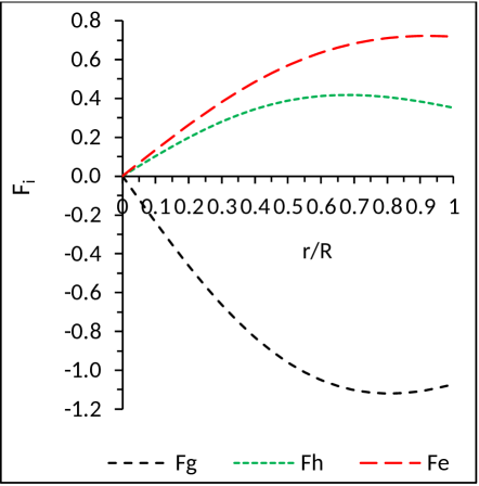
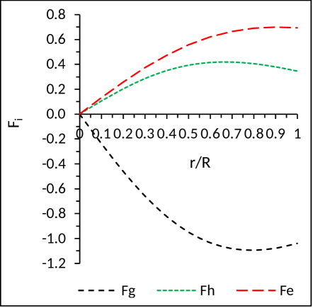
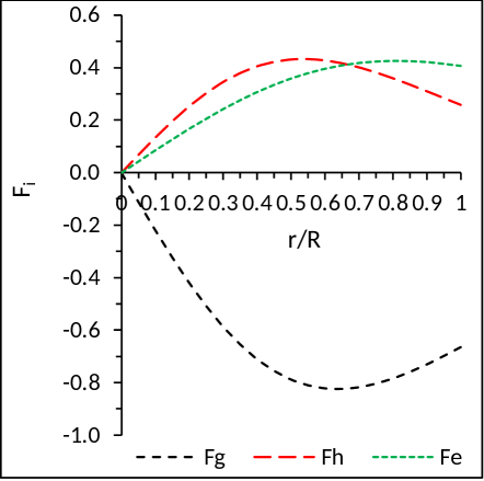
From the plot for TOV equation in Fig. 6 it can be observed that the system is in static equilibrium. The sum of all the forces, like gravitational, hydrostatic and electric forces, are zero. It is interesting to note from Fig. 6 that the gravitational force is counter balanced by the joint action of hydrostatic and electric forces.
5.5 Effective mass-radius relation
For physically valid models, the ratio of the mass to the radius of a compact star models can not be arbitrarily large. Buchdahl Buchdahl1959 has imposed a stringent restriction on the mass-to-radius ratio that for the perfect fluid model it should be . However, Böhmer and Harko Boehmer2007 have given the generalized expression of lower bound for charged compact object as follows:
| (49) |
The upper bound of the mass for charged fluid sphere was generalized by Andréasson Andreasson and proved that
| (50) |
We, therefore, conclude from the above two conditions that must satisfy the following inequality
| (51) |
In this model, the effective gravitational mass has the following form
| (52) |
which can finally be expressed as
| (53) |
5.6 Surface red-shift
We define the compactification factor as
| (54) |
The surface redshift corresponding to the above compactness factor is obtained as
| (55) |
| Compact stars | ||||
|---|---|---|---|---|
| Her. X-1 | 7.36x | 7.32x | 7.29x | 7.29x |
| RXJ 1856-37 | 9.56x | 9.47x | 9.43x | 9.44x |
| SAX J1808.4- 3658(SS2) | 15.59x | 15.25x | 15.10x | 15.08x |
| SAX J1808.4- 3658(SS1) | 11.74x | 11.50x | 11.40x | 11.39x |
| Compact star | ||||||
|---|---|---|---|---|---|---|
| Her. X-1 | 0.98 | 6.7 | 0.1000 | 0.03272 | 0.003260 | 0.0003258 |
| RXJ 1856-37 | 0.9048 | 6.003 | 0.10437 | 0.03414 | 0.003400 | 0.0003400 |
| SAX J1808.4- 3658(SS2) | 1.3232 | 6.33 | 0.1893 | 0.06108 | 0.006048 | 0.0006042 |
| SAX J1808.4- 3658(SS1) | 1.435 | 7.07 | 0.1779 | 0.05750 | 0.005700 | 0.0005695 |
In Table 3 we have shown which are very required as all the equations are dependent on , specially Eq. (35). As we know that for each different star the ratio is fixed, so for this purpose we suppose the value of to determine the ratio from Eq. (35). The feature of is shown in Fig. 7.
| Compact star | Central density | Surface density | Central pressure | ||
|---|---|---|---|---|---|
| () | () | () | |||
| Her. X-1 | 2.0892 | 1.0742 | 8.4453 | 0.432 | |
| RXJ 1856-37 | 2.6964 | 1.3588 | 1.1487 | 0.444 | |
| SAX J1808.4-3658(SS2) | 3.8651 | 1.4409 | 3.4786 | 0.616 | |
| SAX J1808.4-3658(SS1) | 2.9626 | 1.1407 | 2.4628 | 0.598 |
5.7 Electric charge
The amount of charge at the centre and boundary for different stars are given in Table 5. Also, from Fig. 8, it is clear that the charge profile is minimum at the centre and monotonically increasing away from the centre, however it acquires the maximum value at the boundary of the stars. To convert the amount of charge in Coulomb, every value should be multiplied by a factor in the Table 5.
| Her. X-1 | RXJ 1856-37 | SAX J1808.4-3658(SS1) | SAX J1808.4-3658(SS2) | |
|---|---|---|---|---|
| 0.0 | 0.0 | 0.0 | 0.0 | 0.0 |
| 0.2 | 0.0126 | 0.0117 | 0.0189 | 0.0174 |
| 0.4 | 0.098 | 0.0905 | 0.1466 | 0.135 |
| 0.6 | 0.3144 | 0.2902 | 0.468 | 0.4314 |
| 0.8 | 0.6971 | 0.6426 | 1.0253 | 0.9453 |
| 1.0 | 1.2564 | 1.1562 | 1.8141 | 1.6706 |
6 Conclusion
We have investigated for a new stellar model with spherically symmetric matter distribution under the Einstein-Maxwell spacetime. It is observed that the model represents a compact star of embedding class one. The solutions obtain here are general in their nature having the following two specific features:
(i) The metric becomes flat and also the expressions for the pressure, energy density and electric charge become zero in all the cases if we consider the constant , which shows that our solutions represent the so-called ‘electromagnetic mass model’ Lorentz1904 .
(ii) The metric function , for the limit tends to infinity, converts to , which is the same as considered by Maurya et al. Maurya2015a .
We have also studied several physical aspects of the model and find that all the features are acceptable within the expected demand of the contemporary theoretical works and observational evidences. Some salient features of these physical behaviour of our models are as follows:
(1) Regularity condition: We have discussed the situations in the following cases:
(i) Potentials at the centre : From Eqs. (17) and (18), we observe that the metric potentials at the centre becomes and . This implies that metric potentials are singularity free and positive at the centre. However, both are monotonically increasing function (Fig. 1).
(ii) Pressure at the centre : From Eq. (21), one can obtain , where and are positive. The pressure should be positive at the centre and this implies that .
(iii) Density at the centre : From Eq. (22), we get the central density which must be positive at the centre. Since is positive then is also positive due to positivity of . We know that , where , , are all positive. This implies that is also positive.
(2) Casuality and Well behaved condition: The speed of sound as suggested by Canuto Canuto satisfies in the presented compact star model as is evident from Fig. 4.
It can be observed from Fig. 4 that the velocity of sound starts decreasing from and this clearly indicates that the solution is well behaved from onwards and it seems possible to get a reasonable model even when tends to infinity.
(3) Energy Conditions: In our model all the energy conditions, viz. NEC, SEC and WEC, satisfy simultaneously at all the interior points of the star.
(4) Generalized TOV equation: The generalized Tolman-Oppenheimer-Volkoff (TOV) equation Tolman1939 ; Oppenheimer1939 satisfies here and indicates that the model is in static equilibrium under the interaction between the gravitational, hydrostatic and electric forces.
(5) Effective mass-radius relation: We have verified that the Buchdahl Buchdahl1959 condition satisfies in our model within the stipulated range as can be observed from the Table 4.
(6) Surface red-shift: The surface redshift in the present model is found to be satisfactory as can be seen from Fig. 7.
(7) Electric charge: The amount of charge at the centre and boundary for different stars can be found from Table 5. Fig. 8 depicts that the charge is minimum at the centre and monotonically increasing away from the centre, however it acquires the maximum value at the boundary of the stars.
As a final comment, however, it is to be justified to consider several other aspects of embedding class 1 metric and further investigations on the corresponding model for compact stars as far as ultra-modern observational evidences are concerned.
Acknowledgments
SKM acknowledges support from the authority of University of Nizwa, Nizwa, Sultanate of Oman. Also SR is thankful to the authority of The Institute of Mathematical Sciences, Chennai, India for providing Associateship under which a part of this work was carried out there.
References
- (1) H.A. Lorentz, Proc. Acad. Sci. Amsterdam 6 (1904) (Reprinted in: Einstein et al., “The Principle of Relativity”, Dover, INC, p. 24, 1952)
- (2) S.K. Maurya, Y.K. Gupta, S. Ray, S. Roy Chowdhury, Eur. Phys. J. C 75 389 (2015)
- (3) A. Friedmann, Zeit. Physik 10, 377 (1922)
- (4) H.P. Robertson, Rev. Mod. Phys. 5, 62 (1933)
- (5) G. Lema tre, Annal. Soc. Sci. Brux. 53, 51 (1933)
- (6) R.R. Kuzeev, Gravit. Teor. Otnosit. 16, 93 (1980)
- (7) K. Schwarzschild, Phys.-Math. Klasse, 189 (1916)
- (8) M. Kohler, K.L. Chao, Z. Naturforsch. Ser. A 20, 1537 (1965)
- (9) J.A. Wheeler, Geometrodynamics (p. 25, Academic, New York, 1962)
- (10) R.P. Feynman, R.B. Leighton and M. Sands, The Feynman Lectures on Physics , Addison-Wesley, Palo Alto, Vol. II, Chap. 28 (1964)
- (11) P.S. Florides, Proc. R. Soc. (Lond.) Ser. A 337, 529 (1974)
- (12) R.N. Tiwari, J.R. Rao, R.R. Kanakamedala, Phys. Rev. D 30, 489 (1984).
- (13) R. Gautreau, Phys. Rev. D 31, 1860 (1985).
- (14) Ø. Grøn, Phys. Rev. D 31, 2129 (1985).
- (15) . Grn, Gen. Relativ. Gravit. 18, 591 (1986)
- (16) F.I. Cooperstock, N. Rosen, Int. J. Theor. Phys. 28, 423 (1989)
- (17) R.N. Tiwari, J.R. Rao, S. Ray, Astrophys. Space Sci. 178, 119 (1991)
- (18) R.N. Tiwari, S. Ray, Astrophys. Space Sci. 180, 143 (1991)
- (19) R.N. Tiwari, S. Ray, Astrophys. Space Sci. 182, 105 (1991)
- (20) S. Ray, D. Ray, R.N. Tiwari, Astrophys. Space Sci. 199, 333 (1993)
- (21) R.N. Tiwari, S. Ray, Gen. Relativ. Gravit. 29, 683 (1997)
- (22) F. Wilczek, Phys. Today 52, 11 (1999)
- (23) S. Ray, Astrophys. Space Sci. 280, 345 (2002)
- (24) S. Ray, B. Das, Astrophys. Space Sci. 282, 635 (2002)
- (25) S. Ray, B. Das, Mon. Not. R. Astron. Soc. 349, 1331 (2004)
- (26) S. Ray, S Bhadra, Phys. Lett. A 322, 150 (2004)
- (27) S. Ray, Int. J. Mod. Phys. D 15 917 (2006)
- (28) S. Ray, B. Das, F. Rahaman, S. Ray, Int. J. Mod. Phys. D 16, 1745 (2007)
- (29) A.L. Mehra, Gen. Relativ. Gravit. 12, 187 (1980)
- (30) B. Kuchowicz, Acta Phys. Pol. 33, 541 (1968)
- (31) K.D. Krori, J. Barua, J. Phys. A 8, 508 (1975)
- (32) K.R. Karmarkar, Proc. Ind. Acad. Sci.A 27, 56 (1948)
- (33) S.N. Pandey, S.P. Sharma, Gen. Relativ. Gravit. 14, 113 (1982)
- (34) K. Lake, Phys. Rev. D 67, 104015 (2003)
- (35) M.S.R. Delgaty, K. Lake, Comput. Phys. Commun. 115, 395 (1998)
- (36) S.K. Maurya, Y.K. Gupta, Astrophys Space Sci. 334, 301 (2011)
- (37) F. Rahaman, S.A.K. Jafry, K. Chakraborty, Phys. Rev. D 82, 104055 (2010)
- (38) C.W. Misner, D.H. Sharp: Phys. Rev. B 136, 571 (1964)
- (39) V. Canuto, In Solvay Conf. on Astrophysics and Gravitation, Brussels (1973)
- (40) R.C. Tolman, Phys. Rev. 55, 364 (1939)
- (41) J.R. Oppenheimer, G.M. Volkoff, Phys. Rev. 55 374 (1939)
- (42) S.K. Maurya, Y.K. Gupta, S. Ray, arXiv: 1502.01915, [gr-qc] (2015)
- (43) H.A. Buchdahl, Phys. Rev. 116 1027 (1959).
- (44) C.G. Böhmer and T. Harko, Gen. Relativ. Gravit. 39 757 (2007).
- (45) H. Andréasson, Commun. Math. Phys. 288, 715 (2009)