A new point of NP-hardness for 2-to-1 Label Cover

In this paper, we focus on proving $\mathsf{NP}$-hardness for the $2$-to-$1$ Label Cover problem. To the best of our knowledge, no explicit $\mathsf{NP}$-hardness factor has previously been stated in the literature. However it is “folklore” that one can obtain an explicit one for label set sizes $3$ & $6$ by performing the “constraint-variable” reduction on an $\mathsf{NP}$-hardness result for $3$-coloring (more precisely, Max-$3$-Colorable-Subgraph). The best known hardness for $3$-coloring is due to Guruswami and Sinop [GS09], who showed a factor $\frac{32}{33}$-hardness via a somewhat involved gadget reduction from the $3$-query adaptive PCP result of [GLST98]. This yields $\mathsf{NP}$-hardness of $(1,\frac{65}{66}+\epsilon)$-approximating $2$-to-$1$ Label Cover with label set sizes $3$ & $6$. It is not known how to take advantage of larger label set sizes. On the other hand, for label set sizes $2$ & $4$ it is known that satisfying $2$-to-$1$ Label Cover instances can be found in polynomial time.

The main result of our paper gives an improved hardness result:

Let us describe the high-level idea behind our result. The folklore constraint-variable reduction from $3$-coloring to $2$-to-$1$ Label Cover would work just as well if we started from “$3$-coloring with literals” instead. By this we mean the CSP with domain $\mathbbm{Z}_{3}$ and constraints of the form “$v_{i}-v_{j}\neq c\pmod{3}$”. Starting from this CSP — which we call $\textsf{2NLin}(\mathbbm{Z}_{3})$ — has two benefits: first, it is at least as hard as $3$-coloring and hence could yield a stronger hardness result; second, it is a bit more “symmetrical” for the purposes of designing reductions. We obtain the following hardness result for $\textsf{2NLin}(\mathbbm{Z}_{3})$.

Thus, we need a different proof to derive a hardness result from this function-in-the-middle test. We first were able to accomplish this by an analysis similar to the Fourier-based proof of $2\mathsf{Lin}(\mathbbm{Z}_{2})$ hardness given in Appendix F of [OW12]. Just as that proof “reveals” that the function-in-the-middle $2\mathsf{Lin}(\mathbbm{Z}_{2})$ test can be equivalently thought of as Håstad’s $3\mathsf{Lin}(\mathbbm{Z}_{2})$ test composed with the $3\mathsf{Lin}(\mathbbm{Z}_{2})$-to-$2\mathsf{Lin}(\mathbbm{Z}_{2})$ gadget of [TSSW00], our proof for the $\textsf{2NLin}(\mathbbm{Z}_{3})$ function-in-the-middle test revealed it to be the composition of a function test for a certain four-variable CSP with a gadget. We have called the particular four-variable CSP 4-Not-All-There, or 4NAT for short. Because it is a $4$-CSP, we are able to prove the following $\mathsf{NP}$-hardness of approximation result for it using a classic, Håstad-style Fourier-analytic proof.

We leave to Section 2 most of the definitions, including those of the CSPs we use. The heart of the paper is in Section 3, where we give both the $\textsf{2NLin}(\mathbbm{Z}_{3})$ and 4NAT function tests, explain how one is derived from the other, and then perform the Fourier analysis for the 4NAT test. The actual hardness proof for 4NAT is presented in Section 4, and it follows mostly the techniques put in place by Håstad in [Hås01].

An instance $\mathcal{I}$ of a constraint satisfaction problem (CSP) is a set of variables $V$, a set of labels $D$, and a weighted list of constraints on these variables. We assume that the weights of the constraints are nonegative and sum to 1. The weights therefore induce a probability distribution on the constraints. Given an assignment to the variables $f:V\rightarrow D$, the value of $f$ is the probability that $f$ satisfies a constraint drawn from this probability distribution. The optimum of $\mathcal{I}$ is the highest value of any assignment. We say that an $\mathcal{I}$ is $s$-satisfiable if its optimum is at least $s$. If it is 1-satisfiable we simply call it satisfiable.

We define a CSP $\mathcal{P}$ to be a set of CSP instances. Typically, these instances will have similar constraints. We will study the problem of $(c,s)$-deciding $\mathcal{P}$. This is the problem of determining whether an instance of $\mathcal{P}$ is at least $c$-satisfiable or less than $s$-satisfiable. Related is the problem of $(c,s)$-approximating $\mathcal{P}$, in which one is given a $c$-satisfiable instance of $\mathcal{P}$ and asked to find an assignment of value at least $s$. It is easy to see that $(c,s)$-deciding $\mathcal{P}$ is at least as easy as $(c,s)$-approximating $\mathcal{P}$. Thus, as all our hardness results are for $(c,s)$-deciding CSPs, we also prove hardness for $(c,s)$-approximating these CSPs.

We now state the three CSPs that are the focus of our paper.

A typical way of relating two separate CSPs is by constructing a gadget reduction which translates from one to the other. A gadget reduction from $\mathsf{CSP}_{1}$ to $\mathsf{CSP}_{2}$ is one which maps any $\mathsf{CSP}_{1}$ constraint into a weighted set of $\mathsf{CSP}_{2}$ constraints. The $\mathsf{CSP}_{2}$ constraints are over the same set of variables as the $\mathsf{CSP}_{1}$ constraint, plus some new, auxiliary variables (these auxiliary variables are not shared between constraints of $\mathsf{CSP}_{1}$). We require that for every assignment which satisfies the $\mathsf{CSP}_{1}$ constraint, there is a way to label the auxiliary variables to fully satisfy the $\mathsf{CSP}_{2}$ constraints. Furthermore, there is some parameter $0<\gamma<1$ such that for every assignment which does not satisfy the $\mathsf{CSP}_{1}$ constraint, the optimum labeling to the auxiliary variables will satisfy exactly $\gamma$ fraction of the $\mathsf{CSP}_{2}$ constraints. Such a gadget reduction we call a $\gamma$-gadget-reduction from $\mathsf{CSP}_{1}$ to $\mathsf{CSP}_{2}$. The following proposition is well-known:

We note that the notation $\gamma$-gadget-reduction is similar to a piece of notation employed by [TSSW00], but the two have different (though related) definitions.

Let $\omega=e^{2\pi i/3}$ and set $U_{3}=\{\omega^{0},\omega^{1},\omega^{2}\}$. For $\alpha\in\mathbbm{Z}_{3}^{n}$, consider the Fourier character $\chi_{\alpha}:\mathbbm{Z}_{3}^{n}\rightarrow U_{3}$ defined as $\chi_{\alpha}(x)=\omega^{\alpha\cdot x}$. Then it is easy to see that $\mathop{\bf E\/}[\chi_{\alpha}({\boldsymbol{x}})\overline{\chi_{\beta}({\boldsymbol{x}})}]={\bf 1}[\alpha=\beta]$, where here and throughout ${\boldsymbol{x}}$ has the uniform probability distribution on $\mathbbm{Z}_{3}^{n}$ unless otherwise specified.. As a result, the Fourier characters form an orthonormal basis for the set of functions $f:\mathbbm{Z}_{3}^{n}\rightarrow U_{3}$ under the inner product $\langle f,g\rangle=\mathop{\bf E\/}[f({\boldsymbol{x}})g({\boldsymbol{x}})]$; i.e.,

where the $\hat{f}(\alpha)$’s are complex numbers defined as $\hat{f}(\alpha)=\mathop{\bf E\/}[f({\boldsymbol{x}})\overline{\chi_{\alpha}({\boldsymbol{x}})}]$. For $\alpha\in\mathbbm{Z}_{3}^{n}$, we use the notation $|\alpha|$ to denote $\sum\alpha_{i}$ and $\#\alpha$ to denote the number of nonzero coordinates in $\alpha$. When $d$ is clear from context and $\alpha\in\mathbbm{Z}_{3}^{dK}$, define $\pi_{3}(\alpha)\in\mathbbm{Z}_{3}^{K}$ so that $(\pi_{3}(\alpha))_{i}\equiv|\alpha[i]|\pmod{3}$ (recall the notation $\alpha[i]$ from the beginning of this section).

We have Parseval’s identity: for every $f:\mathbbm{Z}_{3}^{n}\rightarrow U_{3}$ it holds that $\sum_{\alpha\in\mathbbm{Z}_{3}^{n}}|\hat{f}(\alpha)|^{2}=1$. Note that this implies that $|\hat{f}(\alpha)|\leq 1$ for all $\alpha$, as otherwise $\hat{f}(\alpha)^{2}$ would be greater than 1. A function $f:\mathbbm{Z}_{3}^{n}\rightarrow\mathbbm{Z}_{3}$ is said to be folded if for every $x\in\mathbbm{Z}_{3}^{n}$ and $c\in\mathbbm{Z}_{3}$, it holds that $f(x+c)=f(x)+c$, where $(x+c)_{i}=x_{i}+c$.

Now that we have shown that 2NLin hardness results translate into 2-to-1 Label Cover hardness results, we present our 2NLin function test. Even though we don’t directly use it, it helps explain how we were led to consider the 4NAT CSP. Furthermore, the Fourier analysis that we eventually use for the 4NAT Test could instead be performed directly on the 2NLin Test without any direct reference to the 4NAT predicate. The test is:

2NLin Test

Given folded functions $f:\mathbbm{Z}_{3}^{K}\rightarrow\mathbbm{Z}_{3}$, $g,h:\mathbbm{Z}_{3}^{dK}\rightarrow\mathbbm{Z}_{3}$:

• •

  Let ${\boldsymbol{x}}\in\mathbbm{Z}_{3}^{K}$ and $\boldsymbol{y}\in\mathbbm{Z}_{3}^{dK}$ be independent and uniformly random.

• •

  For each $i\in[K],j\in[d]$, select $(\boldsymbol{z}[i])_{j}$ independently and uniformly from the elements of $\mathbbm{Z}_{3}\setminus\{{\boldsymbol{x}}_{i},(\boldsymbol{y}[i])_{j}\}$.

• •

  With probability $\frac{1}{4}$, test $f({\boldsymbol{x}})\neq h(\boldsymbol{z})$; with probability $\frac{3}{4}$, test $g(\boldsymbol{y})\neq h(\boldsymbol{z})$.

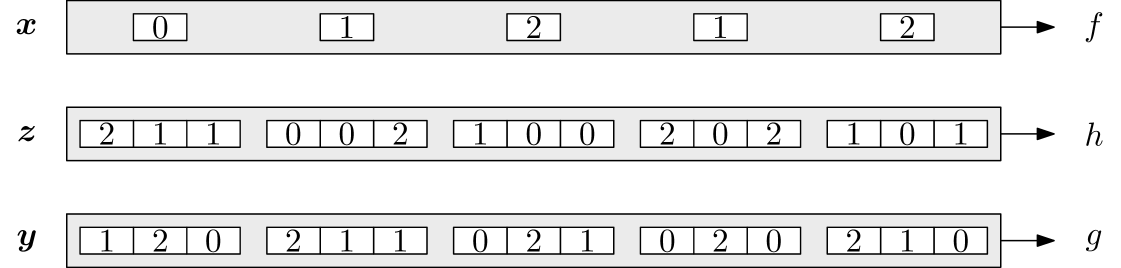
Above is an illustration of the test. We remark that for any given block $i$, $z[i]$ determines $x_{i}$ (with very high probability), because as soon as $z[i]$ contains two distinct elements of $\mathbbm{Z}_{3}$, $x_{i}$ must be the third element of $\mathbbm{Z}_{3}$. Notice also that in every column of indices, the input to $h$ always differs from the inputs to both $f$ and $g$. Thus, “matching dictator” assignments pass the test with probability $1$. (This is the case in which $f(x)=x_{i}$ and $g(y)=(y[i])_{j}$ for some $i\in[K]$, $j\in[d]$.) On the other hand, if $f$ and $g$ are “nonmatching dictators”, then they succeed with only $\frac{11}{12}$ probability. This turns out to be essentially optimal among functions $f$ and $g$ without “matching influential coordinates/blocks”. We will obtain the following theorem:

Before proving this, let us further discuss the 2NLin test. Given ${\boldsymbol{x}}$, $\boldsymbol{y}$, and $\boldsymbol{z}$ from the 2NLin test, consider the following method of generating two additional strings $\boldsymbol{y}^{\prime},\boldsymbol{y}^{\prime\prime}\in\mathbbm{Z}_{3}^{dK}$ which represent $h$’s “uncertainty” about $\boldsymbol{y}$. For $j\in[d]$, if ${\boldsymbol{x}}_{i}=(\boldsymbol{y}[i])_{j}$, then set both $(\boldsymbol{y}^{\prime}[i])_{j}$ and $(\boldsymbol{y}^{\prime\prime}[i])_{j}$ to the lone element of $\mathbbm{Z}_{3}\setminus\{{\boldsymbol{x}}_{i},(\boldsymbol{z}[i])_{j}\}$. Otherwise, set one of $(\boldsymbol{y}^{\prime}[i])_{j}$ or $(\boldsymbol{y}^{\prime\prime}[i])_{j}$ to ${\boldsymbol{x}}_{i}$, and the other one to $(\boldsymbol{y}[i])_{j}$. It can be checked that $\textsf{TwoPair}({\boldsymbol{x}}_{i},(\boldsymbol{y}[i])_{j},(\boldsymbol{y}^{\prime}[i])_{j},(\boldsymbol{y}^{\prime\prime}[i])_{j})=1$, a more stringent requirement than satisfying 4NAT. In fact, the marginal distribution on these four variables is a uniformly random assignment that satisfies the TwoPair predicate. Conditioned on ${\boldsymbol{x}}$ and $\boldsymbol{z}$, the distribution on $\boldsymbol{y}^{\prime}$ and $\boldsymbol{y}^{\prime\prime}$ is identical to the distribution on $\boldsymbol{y}$. To see this, first note that by construction, neither $(\boldsymbol{y}^{\prime}[i])_{j}$ nor $(\boldsymbol{y}^{\prime\prime}[i])_{j}$ ever equals $(\boldsymbol{z}[i])_{j}$. Further, because these indices are distributed as uniformly random satisfying assignments to TwoPair, $\mathop{\bf Pr\/}[(\boldsymbol{y}^{\prime}[i])_{j}=x_{i}]=\mathop{\bf Pr\/}[(\boldsymbol{y}^{\prime\prime}[i])_{j}=x_{i}]=\frac{1}{3}$, which matches the corresponding probability for $\boldsymbol{y}$. Thus, as $\boldsymbol{y}$, $\boldsymbol{y}^{\prime}$, and $\boldsymbol{y}^{\prime\prime}$ are distributed identically, we may rewrite the test’s success probability as:

This is because if 4NAT fails to hold on the tuple $(f({\boldsymbol{x}}),g(\boldsymbol{y}),g(\boldsymbol{y}^{\prime}),g(\boldsymbol{y}^{\prime\prime}))$, then $h(\boldsymbol{z})$ can disagree with at most $3$ of them.

At this point, we have removed $h$ from the test analysis and have uncovered what appears to be a hidden 4NAT test inside the 2NLin Test: simply generate four strings ${\boldsymbol{x}}$, $\boldsymbol{y}$, $\boldsymbol{y}^{\prime}$, and $\boldsymbol{y}^{\prime\prime}$ as described earlier, and test $\textsf{4NAT}(f({\boldsymbol{x}}),g(\boldsymbol{y}),g(\boldsymbol{y}^{\prime}),g(\boldsymbol{y}^{\prime\prime}))$. With some renaming of variables, this is exactly what our 4NAT Test does:

4NAT Test

Given folded functions $f:\mathbbm{Z}_{3}^{K}\rightarrow\mathbbm{Z}_{3}$, $g:\mathbbm{Z}_{3}^{dK}\rightarrow\mathbbm{Z}_{3}$:

• •

  Let ${\boldsymbol{x}}\in\mathbbm{Z}_{3}^{K}$ be uniformly random.

• •

  Select $\boldsymbol{y},\boldsymbol{z},\boldsymbol{w}$ as follows: for each $i\in[K],j\in[d]$, select $((\boldsymbol{y}[i])_{j},(\boldsymbol{z}[i])_{j},(\boldsymbol{w}[i])_{j})$ uniformly at random from the elements of $\mathbbm{Z}_{3}$ satisfying $\textsf{TwoPair}({\boldsymbol{x}}_{i},(\boldsymbol{y}[i])_{j},(\boldsymbol{z}[i])_{j},(\boldsymbol{w}[i])_{j})$.

• •

  Test $\textsf{4NAT}(f({\boldsymbol{x}}),g(\boldsymbol{y}),g(\boldsymbol{z}),g(\boldsymbol{w}))$.

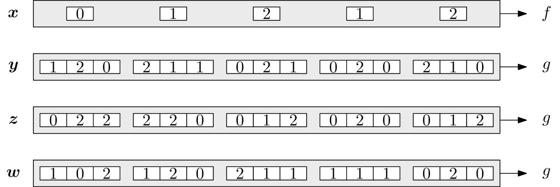
Above is an illustration of this test. In this illustration, the strings $\boldsymbol{z}$ and $\boldsymbol{w}$ were derived from the strings in Figure 1 using the process detailed above for generating $\boldsymbol{y}^{\prime}$ and $\boldsymbol{y}^{\prime\prime}$. Note that each column is missing one of the elements of $\mathbbm{Z}_{3}$, and that each column satisfies the TwoPair predicate. Because satisfying TwoPair implies satisfying 4NAT, matching dictators pass this test with probability $1$. On the other hand, it can be seen that nonmatching dictators pass the test with probability $\frac{2}{3}$. In the next section we show that this is optimal among functions $f$ and $g$ without “matching influential coordinates/blocks”.

(As one additional remark, our 2NLin Test is basically the composition of the 4NAT Test with the gadget from Lemma 3.1. In this test, if we instead performed the $f({\boldsymbol{x}})\neq h(\boldsymbol{z})$ test with probability $\frac{1}{3}$ and the $g(\boldsymbol{y})\neq h(\boldsymbol{z})$ test with probability $\frac{2}{3}$, then the resulting test would basically be the composition of a 3NLin test with a suitable 3NLin-to-2NLin gadget.)

Let $\omega=e^{2\pi i/3}$, and set $U_{3}=\{\omega^{0},\omega^{1},\omega^{2}\}$. In what follows, we identify $f$ and $g$ with the functions $\omega^{f}$ and $\omega^{g}$, respectively, whose range is $U_{3}$ rather than $\mathbbm{Z}_{3}$. Set $L=dK$. The remainder of this section is devoted to the proof of the following lemma:

The first step is to “arithmetize” the 4NAT predicate. It is not hard to verify that

Using the symmetry between $\boldsymbol{y}$, $\boldsymbol{z}$, and $\boldsymbol{w}$, we deduce

In the second term in the RHS of (2) we in fact have $\mathop{\bf E\/}[f({\boldsymbol{x}})\overline{g(\boldsymbol{y})}]=0$. This is because ${\boldsymbol{x}}$ and $\boldsymbol{y}$ are independent, and hence $\mathop{\bf E\/}[f({\boldsymbol{x}})\overline{g(\boldsymbol{y})}]=\mathop{\bf E\/}[f({\boldsymbol{x}})]\mathop{\bf E\/}[\overline{g(\boldsymbol{y})}]=0\cdot 0$ since $f$ and $g$ are folded. Regarding the third term of the RHS in (2), this also turns out to be $0$ by virtue of $g$ being folded. This can be proven using a Fourier-analytic argument; we present here an alternate combinatorial argument:

Equation (2) has now been reduced to

As $g(\boldsymbol{y})g(\boldsymbol{z})g(\boldsymbol{w})$ is always in $U_{3}$, $\Re\mathop{\bf E\/}[g(\boldsymbol{y})g(\boldsymbol{z})g(\boldsymbol{w})]$ is always at least $-\frac{1}{2}$. Therefore,

It remains to handle the $\mathop{\bf E\/}[f({\boldsymbol{x}})g(\boldsymbol{y})g(\boldsymbol{z})]$ term, which is the subject of our next lemma. This is done through a standard argument in the style of Håstad [Hås01].

References

- [ABS10] Sanjeev Arora, Boaz Barak, and David Steurer. Subexponential algorithms for Unique Games and related problems. In Proceedings of the 51st Annual IEEE Symposium on Foundations of Computer Science, pages 563–572, 2010.
- [AM09] Per Austrin and Elchanan Mossel. Approximation resistant predicates from pairwise independence. Computational Complexity, 18(2):249–271, 2009.
- [BRS11] Boaz Barak, Prasad Raghavendra, and David Steurer. Rounding semidefinite programming hierarchies via global correlation. In Proceedings of the 52nd Annual IEEE Symposium on Foundations of Computer Science, 2011.
- [DMR09] Irit Dinur, Elchanan Mossel, and Oded Regev. Conditional hardness for approximate coloring. SIAM Journal on Computing, 39(3):843–873, 2009.
- [FJ97] Alan Frieze and Mark Jerrum. Improved approximation algorithms for MAX k-CUT and MAX BISECTION. Algorithmica, 18(1):67–81, 1997.
- [FK94] Uriel Feige and Joe Kilian. Two prover protocols: low error at affordable rates. In Proceedings of the 26th Annual ACM Symposium on Theory of Computing, pages 172–183, 1994.
- [GKO+10] Venkatesan Guruswami, Subhash Khot, Ryan O’Donnell, Preyas Popat, Madhur Tulsiani, and Yi Wu. SDP gaps for 2-to-1 and other Label-Cover variants. In Proceedings of the 37th Annual International Colloquium on Automata, Languages and Programming, pages 617–628, 2010.
- [GLST98] Venkatesan Guruswami, Daniel Lewin, Madhu Sudan, and Luca Trevisan. A tight characterization of NP with 3 query PCPs. In Proceedings of the 39th Annual IEEE Symposium on Foundations of Computer Science, pages 8–17, 1998.
- [GS09] Venkatesan Guruswami and Ali Kemal Sinop. Improved inapproximability results for Maximum k-Colorable Subgraph. In Proceedings of the 12th Annual International Workshop on Approximation Algorithms for Combinatorial Optimization Problems, pages 163–176, 2009.
- [GS11] Venkatesan Guruswami and Ali Sinop. Lasserre hierarchy, higher eigenvalues, and approximation schemes for quadratic integer programming with PSD objectives. In Proceedings of the 52nd Annual IEEE Symposium on Foundations of Computer Science, 2011.
- [GW04] Michel X. Goemans and David P. Williamson. Approximation algorithms for MAX-3-CUT and other problems via complex semidefinite programming. J. Comput. Syst. Sci., 68(2):442–470, 2004.
- [Hås01] Johan Håstad. Some optimal inapproximability results. Journal of the ACM, 48(4):798–859, 2001.
- [IP01] Russell Impagliazzo and Ramamohan Paturi. On the complexity of k-SAT. Journal of Computer and System Sciences, 62(2):367–375, 2001.
- [Kho02] Subhash Khot. On the power of unique 2-prover 1-round games. In Proc. 34th ACM Symposium on Theory of Computing, pages 767–775, 2002.
- [KKMO07] Subhash Khot, Guy Kindler, Elchanan Mossel, and Ryan O’Donnell. Optimal inapproximability results for Max-Cut and other -variable CSPs? SIAM Journal on Computing, 37(1):319–357, 2007.
- [KR03] Subhash Khot and Oded Regev. Vertex Cover might be hard to approximate to within . In Proc. 18th IEEE Conference on Computational Complexity, pages 379–386, 2003.
- [MR10] Dana Moshkovitz and Ran Roz. Two-query PCP with subconstant error. Journal of the ACM, 57(5):29, 2010.
- [OW09] Ryan O’Donnell and Yi Wu. Conditional hardness for satisfiable -CSPs. In Proceedings of the 41st Annual ACM Symposium on Theory of Computing, pages 493–502, 2009.
- [OW12] Ryan O’Donnell and John Wright. A new point of NP-hardness for Unique-Games. In Proceedings of the 44th Annual ACM Symposium on Theory of Computing, 2012.
- [Rag08] Prasad Raghavendra. Optimal algorithms and inapproximability results for every CSP? In Proceedings of the 40th Annual ACM Symposium on Theory of Computing, pages 245–254, 2008.
- [Raz95] Ran Raz. A parallel repetition theorem. In Proceedings of the 27th Annual ACM Symposium on Theory of Computing, pages 447–456, 1995.
- [Ste10] David Steurer. Subexponential algorithms for d-to-1 two-prover games and for certifying almost perfect expansion. Available at the author’s website, 2010.
- [TSSW00] Luca Trevisan, Gregory Sorkin, Madhu Sudan, and David Williamson. Gadgets, approximation, and linear programming. SIAM Journal on Computing, 29(6):2074–2097, 2000.
- [Zwi98] Uri Zwick. Approximation algorithms for constraint satisfaction problems involving at most three variables per constraint. In Proceedings of the 9th Annual ACM-SIAM Symposium on Discrete Algorithms, pages 201–210, 1998.