A note on band surgery and the signature of a knot
Abstract.
Band surgery is an operation relating pairs of knots or links in the three-sphere. We prove that if two quasi-alternating knots and of the same square-free determinant are related by a band surgery, then the absolute value of the difference in their signatures is either 0 or 8. This obstruction follows from a more general theorem about the difference in the Heegaard Floer -invariants for pairs of L-spaces that are related by distance one Dehn fillings and satisfy a certain condition in first homology. These results imply that is the only torus knot with square-free that admits a chirally cosmetic banding, i.e. a band surgery operation to its mirror image. We conclude with a discussion on the scarcity of chirally cosmetic bandings.
1991 Mathematics Subject Classification:
57K10, 57K18 (primary), 57R58, 57M12 (secondary)1. Introduction
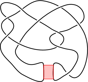
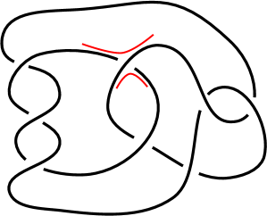
Band surgery is an operation on knots or links in the three-sphere. Let be a link, and let be an embedding of the unit square with . Let denote the link obtained by replacing in with . We say that the link results from band surgery along . See Figure 1 for two examples of band surgeries relating pairs of knots. When and are oriented links and band surgery respects their orientations, the operation is called coherent band surgery. Otherwise, it is called non-coherent. Coherent band surgery converts a knot into a two-component link, whereas non-coherent band surgery converts a knot to another knot.
In this article we are concerned only with non-coherent band surgery operations relating unoriented knots. Elsewhere in the literature non-coherent band surgery is called incoherent band surgery or unoriented banding (e.g. [AK14, Kan16, IJM18]). Band surgery is of interest in low-dimensional topology, in particular in knot theory, and in the study of surfaces in four-manifolds. It is of independent interest in DNA topology; for a more detailed commentary on this perspective, we refer the reader to [LMV19, Section 5] and [MV20], which review the relevance of band surgery to the study of DNA.
In Theorem 4.4, we find a new obstruction to band surgery for quasi-alternating knots via two knot invariants, the determinant and signature of a knot. Both the determinant and the signature of a knot are integer-valued ( is odd and is even) and are determined by the Seifert module [GL78, Tro62]. A quasi-alternating knot is a generalization of an alternating knot due to Ozsváth and Szabó [OS05b]. All alternating knots are quasi-alternating. Two pairs of knots for which Theorem 4.4 applies are shown in Figure 1. Note that any banding relating a pair of knots is necessarily a non-coherent band surgery.
Theorem 4.4.
Let and be a pair of quasi-alternating knots and suppose that for some square-free integer . If there exists a band surgery relating and , then is or .
The determinant of a knot, or more generally the first homology of its branched double cover, can often provide an effective obstruction to the existence of a band surgery relating a pair of knots (see for example [AK14, KM14, Kan16]). However, when a pair of knots have branched double covers with isomorphic first homology (which implies ), such obstructions do not apply. Theorem 4.4 fills this gap in the case where is square-free. Theorem 4.4 is reminiscent of Murasugi’s well-known statement that when and are related by a coherent band surgery [Mur65, Lemma 7.1]. In the case of non-coherent band surgery, the signature of a knot may change by an arbitrary amount. For example, the torus knot , with odd, has signature and is related by a single band surgery operation to the unknot, which has zero signature.
Murasugi also proved that for any knot , the signature controls the determinant of a knot modulo 4 [Mur65, Theorem 5.6]. More precisely, if (resp. 2) modulo 4, then (resp. 3) modulo 4. This immediately implies
for any pair of knots, which provides an explanation for the significance of the numbers 0 and 8 in Theorem 4.4.
Theorem 4.4 follows as a corollary of Theorem 3.5, a more general statement about the Heegaard Floer -invariants of pairs of L-spaces related by integral surgery.
Theorem 3.5.
Let and be L-spaces with , where each is an odd square-free integer. If is obtained by a distance one surgery along any knot in , then
where and denote the unique self-conjugate structures on and .
Heegaard Floer homology is a powerful package of three and four-manifold invariants due to Ozsváth and Szabó [OS03]. An L-space is a rational homology sphere whose Heegaard Floer homology is as simple as possible. One particularly useful Heegaard Floer invariant is the d-invariant of the pair , where is an oriented rational homology sphere and is an element of . The -invariant is a rational number, defined as the minimal grading of a certain submodule of the Heegaard Floer module [OS03]. The reader is referred to [OS03] for an introduction to these invariants. All required background for this note is in sections 2 and 3.
The distance between two Dehn surgery slopes refers to their minimal geometric intersection number. A surgery slope that intersects the meridian of a knot exactly once is called a distance one surgery, or an integral surgery. Given two knots or links related by band surgery, the Montesinos trick [Mon76] implies that their branched double covers may be obtained by distance one Dehn fillings of a three-manifold with torus boundary. To prove Theorem 3.5 we apply the Heegaard Floer mapping cone formula of Ozsváth and Szabó [OS11], and a theorem of Ni and Wu [NW15, Proposition 1.6] which describes the -invariants of a manifold obtained by integral surgery along a null-homologous knot in an L-space in terms of certain integer-valued knot invariants due to Rasmussen [Ras03].

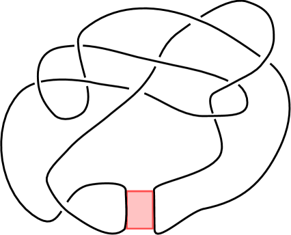
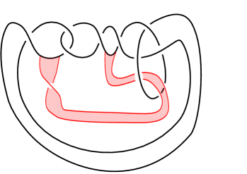
Applications to chirally cosmetic banding. A special case of Theorem 4.4 occurs when a band surgery relates a knot with its mirror image . See Figure 2 for an example. This is called a chirally cosmetic banding. The following is an immediate consequence of Theorem 4.4.
Corollary 4.8.
The only nontrivial torus knot , with square free, admitting a chirally cosmetic banding is .
In section 4, we compare the square-free condition of Theorem 4.4 with the constructive examples of chirally cosmetic bandings given in [IJM18]. Using Monte Carlo simulations we find examples of knots admitting chirally cosmetic bandings. Additionally, in all cases these appear with low probability. Amongst knots of up to eight crossings, the results of our simulations produce three such examples: , , and . The chirally cosmetic banding along was previously not known to exist. An isotopy of the banding is shown in Figure 2 (right).
Organization. In section 2 we introduce notation and establish some prerequisite topological information. Section 3 contains the necessary background in Heegaard Floer homology along with the proof of Theorem 3.5. In section 4 we prove Theorem 4.4, further consider the case of chirally cosmetic pairs and detail the methods of the computer simulations.
2. Preliminaries
2.1. Homological preliminaries
In this section we state some homological preliminaries and set notation. We assume all singular (co)homology groups have coefficients in . Let be a knot in a rational homology sphere , and let denote the complement of in . A slope is an isotopy class of an unoriented simple closed curve on the boundary of . The Dehn filling is the closed, oriented three-manifold obtained by gluing a solid torus to by a homeomorphism which identifies a meridian of to the slope on . The distance between two surgery slopes on is the minimal geometric intersection number of the two curves, denoted for any pair of slopes . In this note we are particularly concerned with surgery slopes which intersect the meridian of exactly once, i.e. distance one surgeries, or integral surgeries.
When is null-homologous, there is a standard choice of a meridian and Seifert longitude on the bounding torus . Here, the meridian is a simple closed curve on that bounds a disk in the solid torus . The preferred longitude is the slope determined by the intersection of a Seifert surface for the knot and . A slope may be written in terms of this standard basis as . Rational Dehn surgery with the surgery coefficient along in is then well-defined, and the result of surgery is denoted by . Indeed, when is null-homologous a homological argument (see for example [Gai18, Lemma 8.1]) shows that , where the -summand is generated by the meridian of . This implies that by a standard Mayer-Vietoris argument. Notice that the Seifert longitude controls the first homology of the Dehn filling, in the sense that .
When is not null-homologous, we have that for some finite group . Let denote the map induced by inclusion in the long exact sequence of the pair ,
The kernel and image of are both rank one. In particular, the kernel of is generated by , where is a primitive class in uniquely determined up to sign. This class determines a well-defined slope in :
Definition 2.1.
The rational longitude is the unique slope in characterized by the property that its image is of finite order in .
When we work with knots that are non-trivial in , we will use the rational longitude to fix a basis for , where now denotes some slope with . Just as with the case of the Seifert longitude for null-homologous knots, the rational longitude also controls the order of the first homology of the filling.
Lemma 2.2.
[Wat12, Lemma 3.2] For any filling slope on ,
| (1) |
where denotes the (necessarily finite) order of the rational longitude in .
In [Wat12, Lemma 3.2], this is proved with a careful analysis of the long exact sequence of the pair. Under the homomorphism , the basis elements and are mapped to and , respectively, where , and are some elements of .
Let us introduce some notation. Consider a decomposition of the finite abelian group as . We will write and for elements written with respect to this decomposition. The notation will stand for the diagonal matrix with -th diagonal entry where are the invariant factors of .
For a filling slope , Watson observes that has a block form presentation matrix
| (2) |
The statement of the lemma then follows.
The reader may notice that the proof of Lemma 2.3 below is adapted from the argument given in [LM17, Theorem 2.4]. In general, we will use the Smith normal form of the presentation matrix (2). Recall that the Smith normal form is a diagonal matrix where . Each , where is the greatest common divisor of the the minors of , and .
Lemma 2.3.
Suppose that where each is an odd square-free integer. If is obtained from by a distance one surgery on a knot in , then is null-homologous and the surgery coefficient is .
Proof.
Let and fix as a basis of , where is some curve dual to the rational longitude . In this basis, filling slopes and yielding and , respectively, may be written as and for some integers and relatively prime to .
By assumption . Applying Lemma 2.2, we have
This implies that . The assumption that is obtained by a distance one surgery along means that is one. Therefore
and so and . After possibly multiplying by to ensure , we may write and . With the change of basis , we can further assume and .
By (1), we have that
If , then bounds in . Because is homologous to the core of the filling torus in , this also means that is null-homologous in . Thus we aim to show that .
Suppose now it is not the case, so that . Consider the presentation matrices and for and ,
where we have multiplied the first column by a unit to ensure that .
We claim that each is a multiple of . If not, then there is some for which there exists a prime power that divides both and , but not . Consider now . Since and we know that for some power . However, if we consider the minor we see (by, say, cofactor expansion at ) that is divisible by at most . Consider now the Smith normal form of . By definition . In particular, is divisible by at most . But this implies , and hence some invariant factor is not square-free. Because we have assumed that the are square-free, we must also have that the are square free. Hence we have reached a contradiction.
Notice that the same argument will apply to the presentation matrix for to show that for . Since and , we also have . With this, we may write
for some integers .
Observe that is trivial if and only if is in the column space of . In particular, since , we have that is in the column space of . Thus there exist integers so that for all .
This then implies is a divisor of , so that for some . We can then write . This shows is in the column space of , which implies is trivial.
We have established that and hence is null-homologous in . Now we take may take the preferred basis on , where is the meridian of and is a Seifert longitude. The condition that the slope yielding is distance one from the meridian implies the slope must in fact be , i.e. the surgery coefficient is .∎
For the remainder of the article, we will assume that is a null-homologous knot in with meridian and longitude . We will be primarily concerned with slopes of the form , for , which are framing curves on the boundary of a neighborhood of . These slopes intersect the meridian once transversely and inherit an orientation from . The notation will denote the result of integral surgery along , and will denote the core of the surgery .
The set is the space of nowhere vanishing vector fields on modulo homotopy outside of a ball. There is a non-canonical correspondence [Tur97]. We write to denote an element of , and write to denote the relative structures on . Note that has an affine identification with , which by excision is isomorphic with . In particular, because is null-homologous and , we may label an element of by , where and . The correspondence is non-canonical, and the labelling that we adopt follows closely to that of [Gai18]. When has odd order, there is a unique self-conjugate structure , distinguished from the others by the requirement that it satisfies (see for example [Section 2][MO07]).
3. Heegaard Floer invariants and the proof of Theorem 3.5
3.1. Heegaard Floer background and the mapping cone formula
We will assume some familiarity with Heegaard Floer homology, referring the reader to [OS03, OS11] for more information. We take all Heegaard Floer complexes with coefficients in the field . One of the main components of the Heegaard Floer package we will use is the -invariant , or correction term, which is a rational number associated to a rational homology sphere . More specifically, given a rational homology sphere , the Heegaard Floer module splits over structures, and in each summand we have
| (3) |
as -modules. The first summand is abbreviated and referred to as the tower. The second summand is a torsion -module. An L-space is a rational homology sphere whose Heegaard Floer homology is a free -module with rank . That is, the torsion summand in (3) vanishes, leaving only a tower in each structure. The -invariant is defined to be the minimal Maslov grading of the tower. The -invariants switch sign under orientation-reversal [OS03].
Associated to and each relative structure in is the knot Floer chain complex [Ras03, OS04, OS11]. The complex is -filtered over with a second filtration induced by the action of the variable . We denote these two filtrations as (algebraic, Alexander). The chain complex also has a homological Maslov grading that we suppress in the notation. Multiplication by decreases the Maslov grading by two and the Alexander filtration by one, and the action of on shifts the Alexander filtration by one, i.e. . Recall that denotes the (class of a) meridian.
As in [OS11], for each in there are complexes and . The complex is . The map is defined in [OS11, Section 2.2], and sends a relative structure to a structure in the target manifold indicated by the subscript. The complex represents the Heegaard Floer complex of a large surgery in a certain structure, where is obtained by Dehn surgery along a framing curve with . There are analogous complexes in the ‘hat’ version of Heegaard Floer homology. In particular we have and . The complexes are related by chain maps
| (4) |
where is the push-off of inside using framing . In [OS11, Theorem 4.1], it is shown that the maps and correspond with a negative definite cobordism equipped with the structures and , respectively, which extend a given structure on . Here, generates and is represented by a capped-off Seifert surface for .
The complexes and each contain a non-torsion summand, i.e. a tower. On homology, each of the maps and induces an endomorphism of the towers, which is multiplication by or for integers and . This defines the knot invariants and , which appeared originally as the local h-invariants in [Ras03]. We remark for later use that when , the corresponding map is identically zero, and similarly implies is zero.
Recall that because is null-homologous, , where the -summand is generated by the meridian of [Gai18, Lemma 8.1]. We write for and . Fixing , we have the subgroup . Because the following properties have appeared in various forms throughout the literature, we provide just a sketch of the proof.
Property 3.1.
Let be a null-homologous knot in a rational homology sphere and let be a self-conjugate structure on . Then the invariants and satisfy:
-
(1)
,
-
(2)
,
-
(3)
for .
(sketch).
Since , we have that . When we fix a self-conjugate structure on on , the statements above relating and are analogous to those for the invariants and , with , for the case of a knot in an integer homology sphere. In particular, Property 1 follows as a direct analogue of [Ras03, Property 7.6] (see also [NW15, Lemma 2.4]). Next, because conjugation changes the sign of the first Chern class and the -action, we may verify using the formulas of [OS08, Section 4.3] that and are conjugate structures on the four-manifold cobordism . This implies Property 2. Finally, 1 and 2 imply 3. See also [HLZ15, Lemmas 2.3-2.5]. ∎
The proof of Theorem 3.5 below will require the mapping cone formula for the Heegaard Floer homology of the integral surgery . We give only a terse review here, sending the reader to Ozsváth and Szabó for details [OS08, OS11]. The generalization of the mapping cone formula specific to rational surgeries on null-homologous knots in L-spaces is also reviewed in [NW15, Gai18]. Note that for our applications, we only require the formulation for integral surgery and ‘hat’ homology.
For each and , sum up the complexes and into
where the first component of each tuple records the index of the summand. Using the maps and from equation (4) above, we define the map by
The mapping cone complex of is denoted . Let us omit the surgery coefficient ‘’ and write the summand of the cone corresponding to the equivalence class of more concisely as .
Theorem 3.2 (Ozsváth and Szabó, [OS11]).
Let . Then there is a relatively-graded isomorphism of groups
| (5) |
Given a structure in , there is a unique structure on which extends over the two-handle cobordism and this defines the projection from to . This projection appears in the following result of Ni and Wu, which will allow us to describe the -invariants of surgeries in terms of the invariants , which crucially, are non-negative integers.
Proposition 3.3 (Proposition 1.6 in [NW15]).
Fix an integer and a self-conjugate structure on an L-space . Let be a null-homologus knot in . Then, there exists a bijective correspondence between and the structures on that extend over such that
| (6) |
where . Here, we assume that .
Proposition 3.3 was originally proved for knots in the three-sphere, but it generalizes immediately to the case of a null-homologous knot in an L-space [NW15], which is the version stated here (see also [LMV19]). The term on the right includes the -invariants of the lens space , which are made explicit in section 3.3.
3.2. Proof of Theorem 3.5
In this section we prove the main result. The requirement that and are L-spaces in the statement of Theorem 3.5 is necessary both to calculate the differences in their -invariants via the surgery formula of Proposition 3.3, and to use the surgery formula directly to determine the value of the invariant . The L-space condition will surface again when we apply Theorem 3.5 to alternating and quasi-alternating knots to obtain Corollary 4.3 and Theorem 4.4. The significance in this context is that quasi-alternating knots have branched double covers that are L-spaces, and there is a connection between the signature of the knot and a certain -invariant of the branched double cover.
Theorem 3.5.
Let and be L-spaces with , where each is an odd square-free integer. If is obtained by a distance one surgery along any knot in , then
| (7) |
where and denote the unique self-conjugate structures on and .
Proof.
Suppose that the homological condition on and is satisfied and that is obtained by a distance one surgery along some knot in . By Lemma 2.3, is null-homologous in and the surgery coefficient is .
Let us first consider when the surgery coefficient is exactly , that is, the filling slope yielding is . Since is a null-homologous knot in an L-space along which there exists an integral surgery to , we may apply Proposition 3.3. In particular, fixing the unique self-conjugate structure on , there is one -structure on that extends over . By Proposition 3.4, is self-conjugate on . But there is a unique self-conjugate structure in . Therefore and by equation (6) we have
| (8) |
Because is the three-sphere, the term vanishes, leaving
| (9) |
where . We claim that is at most one.
Consider the mapping cone formula for the Heegaard Floer chain complex of . Recall that , where we have assumed that . By assumption, both and are L-spaces. Therefore , and for any .
By [OS05a, Proposition 2.1], any sufficiently large surgery will also be an L-space. Since the Heegaard Floer complex of the large surgery (in some -structure) is quasi-isomorphic with the complex , we have that the homology of every summand is torsion-free. In particular,
| (10) |
Thus, the Heegaard Floer homology of is completely determined by the numbers and for each (for this statement, need not be one).
Since the mapping cone splits over , we may restrict our attention to the unique self-conjugate structure on . We have that the ‘hat version’ of the mapping cone formula specialized to surgery along and restricted to on is given by
where we have written in the above diagram for clarity.
Now suppose that . Property 3.1(1) implies that . Property 3.1(2) implies that , and Property 3.1(3) then implies that . Together these imply that the maps and are zero. In particular, and are in the kernel of , and so
By [Gai17, Lemma 12], the map induced by on homology is surjective. Thus the long exact triangle
| (11) |
implies that . But now (10) and (11) imply that
which contradicts that is an L-space. Therefore is at most one. This verifies the claim.
Finally, since , this completes the proof of the theorem in the case that the surgery coefficient is .
If instead the surgery coefficient is , then we may reverse the roles of and . In particular, we consider surgery along a null-homologous knot in yielding the manifold (here is the core of the previous surgery). The above argument applies with the corresponding change in notation. ∎
3.3. Lens spaces and -invariants
The -invariants of lens spaces can be computed with the following recursive formula of Ozsváth and Szabó.
Theorem 3.6 (Proposition 4.8 in [OS03]).
Let be relatively prime integers. Then, there exists an identification such that
| (12) |
for . Here, and are the reductions of and respectively.
It is well-known (see for example [OS06, Section 3.4]), that the self-conjugate structures on the lens space correspond with the set
| (13) |
Note that when is odd, there is a unique self conjugate structure.
Corollary 3.7.
Suppose that is a square-free odd integer. There exists a distance one surgery along any knot in yielding if and only if or .
Proof.
Suppose first that is a square-free odd integer and there exists a distance one surgery along any knot in . Observe that . Because the -invariants change sign under orientation-reversal [OS03], Theorem 3.5 implies that or . By equation (13), the structure corresponds with 0, hence by equation (12) in Theorem 3.6 we have
The -invariant is equal for and equal for .
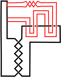
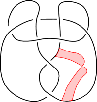
For the reverse direction, note that the branched double cover of is the lens space , and that is the three-sphere. The Montesinos trick implies that any banding along lifts to a distance one Dehn surgery in . In the case , a chirally cosmetic banding from the torus knot to its mirror image exists [Zek15] and is pictured in Figure 2. This band move lifts to a distance one filling taking to . In the case , the relevant banding is induced by a Reidemeister-I move along an unknot (see Figure 3). ∎
4. Band surgery and chirally cosmetic bandings
4.1. Band surgery
A band surgery can be described as a two-string tangle replacement as follows. After possibly isotoping and , the pairs and can be decomposed as
where is the union of the two three-balls and glued along their boundary, the sphere intersects each of and transversely in four points, and , , and are two-string tangles where , and . Note that the “outside” tangle is shared by both of and . In particular, we may isotope and (possibly complicating the outside tangle) until and are the specific two-string rational tangles and , where and correspond to the Conway notation. See [Kaw96, Mur96] for a general discussion of tangles.
The Montesinos trick [Mon76] implies that the branched double covers of knots (or links) related by a band surgery are obtained from distance one Dehn fillings of a three-manifold with torus boundary. This three-manifold is the double cover of the ball branched over . Alternatively, can be described as , where the knot is the lift in the branched cover of the properly embedded arc arising as the core of the band in . The filling slope yielding is the meridian of , and the filling slope yielding is distance one from , meaning and intersect geometrically once.
4.2. Signature-based obstruction to the existence of a band surgery relating two knots
Here we give Theorem 4.4 as a corollary to Theorem 3.5. Recall that the double cover of the three-sphere branched over a knot is a rational homology sphere with of odd order. Ozsváth and Szabó [OS03] defined an integer-valued knot invariant
| (14) |
where is the structure induced by the unique spin structure on . For alternating knots, and for knots of small crossing number, Manolescu and Owens proved that is determined by the signature [MO07].
Theorem 4.1 (Theorems 1.2 and 1.3 in [MO07]).
If the knot is alternating or if has nine or fewer crossings, then .
In [LO15, Theorem 1] Lisca and Owens generalized Theorem 4.1 to quasi-alternating knots. The class of quasi-alternating links generalizes alternating links [OS05b] (see Definition 4.2). Tables of quasi-alternating knots up to 12 crossings can be found in [Jab14].
Definition 4.2.
The set of quasi-alternating links is the smallest set of links satisfying that the unknot is in , and that the set is closed under the following operation. If is a link which admits a diagram with a crossing such that
-
(1)
both resolutions and are in
-
(2)
, , and
-
(3)
,
then is in .
In sum, the signature of a knot is determined by for alternating knots, quasi-alternating knots, and all knots of up to nine-crossings.
Corollary 4.3.
Let and be a pair of quasi-alternating knots and suppose that , where each is a square-free integer. If there exists a band surgery relating and , then is or .
Proof.
If and are quasi-alternating knots, then their branched double covers and are L-spaces [OS05b] and by assumption, . If and differ by a band move, then is obtained by a distance one filling along a knot in (and vice versa). Therefore,
where the first line follows from Theorem 3.5, the second is the definition of in equation (14), and the third line follows from Theorem 4.1 and its generalization [LO15, Theorem 1]. ∎
Note that Theorem 4.4 as stated in the introduction is the specific case of Corollary 4.3 when each is a distinct prime.
Theorem 4.4.
Let and be a pair of quasi-alternating knots and suppose that for some square-free integer . If there exists a band surgery relating and , then is or .
Corollary 4.5.
Excluding , let and be knots of eight or fewer crossings with for a square-free integer. If there exists a banding from to , then or .
Proof.
All knots of up to eight crosings are alternating with the exception of , and . Of these, and are quasi-alternating. So excluding , all knots of up to eight crossings are quasi-alternating. The statement follows from Theorem 4.1. ∎
| Writhe-guided | Rolfsen | Knotplot | |
|---|---|---|---|
Example 4.6.
Recall that the branched double cover of any alternating or quasi-alternating knot is an L-space. The knot is not quasi-alternating (in fact, it is homology-thick) and its branched double cover is not an L-space, hence it is excluded from Corollary 4.5. However, a band surgery relates and . (See Figure 4.) Here, is square-free, and . It is unknown whether the criterion of Corollary 4.5 always holds for .
Example 4.7.
Consider the knots and , for which and . A single band surgery relates and (and hence and ) [Zek15]. Theorem 4.4 implies there is no band surgery relating and . Similarly, consider and . In this case, , while and , so there cannot be a band move relating and . However, Figure 1 illustrates the existence of a band surgery relating and [Zek15]. For the knots in this article, Table 1 provides a nomenclature conversion to Rolfsen [Rol90].
4.3. Chirally cosmetic bandings
A chirally cosmetic banding refers to a non-coherent band surgery taking a knot to its mirror image. The results in the previous section immediately imply the following corollary.
Corollary 4.8.
The only nontrivial torus knot , with square free, admitting a chirally cosmetic banding is .
Proof.
The statement follows from Corollary 3.7 because the branched double cover of is the lens space . Alternatively, we may use Theorem 4.4. Without loss of generality, let . The torus knot has determinant and signature , whereas the mirror has determinant and signature . The absolute value of the difference in signature between and is when and is when . The case of is the unknot. The chirally cosmetic banding for the case is pictured in Figure 2. ∎

The knot in along which there exists a distance one filling yielding descends under the covering involution to the core of the band move from to . As observed in [IJM18], the complement of this knot is the hyperbolic knot complement known as the “figure-eight sibling” and is well known to be amphichieral [MP06, Wee85]. The special symmetries of this manifold suggest an explanation for the uniqueness of ; see [IJM18] for a discussion of this perspective.
In addition to , several constructions of knots admitting chirally cosmetic bandings are described in [IJM18]. These include: the knot , which has determinant 49; Whitehead doubles of achiral knots (i.e. certain satellites), which have determinant 1; and a general construction of certain symmetric unions. A symmetric union is a connected sum of a knot and its mirror image, modified by a tangle replacement such that the resulting diagram admits an axis of mirror symmetry (see Figure 5A). The determinant of a symmetric union is always a square [KT57, Moo16]. Indeed, excluding , all of the examples of knots admitting chirally cosmetic bandings presented in [IJM18] have determinant a square.
Numerical exploration of chirally cosmetic bandings. Corollary 4.8 and the observation that most known constructions of knots admitting chirally cosmetic bandings are symmetric unions suggest that this phenomenon is uncommon. To search for any further chirally cosmetic bandings amongst low crossing knots, we performed computer simulations (described at the end of this section) of non-coherent band surgery along knots. In brief, each knot type was embedded in the cubic lattice. The embeddings were randomized using a Monte Carlo algorithm, where polygons were sampled for each chiral pair and a non-coherent band surgery was performed on each polygon.
| Chiral pairs | Number observed | [] |
|---|---|---|
| 188 | ||
| 1 | ||
| 2677 |
We found chirally cosmetic bandings to be exceedingly rare. Chirally cosmetic bandings were observed in the numerical experiments for only three knot types. The numbers of bandings relating each of these three knots with its mirror image (or vice versa) is given in Table 2.
The band move for was previously reported in [Zek15] and is shown in Figure 2. Only a single band move was observed for the pair and . An isotopy of this banding, discovered only by simulation, is shown in Figure 5B (left). A banding for can more easily be found by hand, as in Figure 5B (right). The banding pictured is a “4-move” in a symmetric union diagram, where a 4-move refers to the replacement of a positive 2-twist with a negative 2-twist. Although is known to admit a symmetric union presentation [Lam19] (see Figure 5A), it is not known to the authors whether a 4-move in such a diagram relates to its mirror. See [IJM18] for a definition of 4-moves.
These observations prompt the following question:
Question 4.9.
Suppose that a pair of knots and are related by band surgery. What is the likelihood that and are of different chirality?
When is a chiral knot and is the mirror of , it is clear what we mean by different chirality. In a forthcoming numerical study propose a method to quantify what it means for arbitrary knots to have different chirality. We expand on the preliminary simulations conducted here and report on the chirality trends with respect to band surgery operations along cubic lattice knots.
Numerical methods. In order to identify candidate pairs for chirally cosmetic bandings, we systematically performed band surgery operations on all nontrivial prime chiral knots with 8 or fewer crossings. Independent simulations were performed for each member of a chiral pair (. Because we excluded fully amphichiral and negative amphichiral knots, a total of 28 knot types were considered. The computer simulations were conducted by adapting software previously developed in our group, the implementation and methods of which are detailed in [SYB+17].
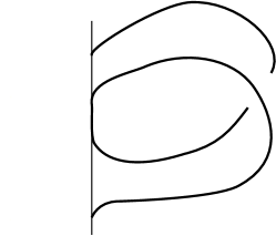
The details of the simulations are as follows. For each knot , we used the BFACF algorithm [MS93] to sample the space of lattice embeddings of . Here a cubic lattice representative of a knot is an embedding of contained in the cubic lattice , where the end points of the line segments are contained in the integer lattice . The BFACF algorithm is a dynamic Monte Carlo method that samples the space of cubic lattice polygons of a specific knot type. In each step of the BFACF Markov chain, the algorithm attempts to locally perturb a polygonal chain as pictured in Figure 6, at a randomly chosen location on edges in the polygon. Note that this can change the length of the polygon by , or . Janse van Rensburg and Whittington showed that the ergodicity classes are the knot types [vRW91], making this a good method for generating large ensembles of lattice embeddings of a specific knot type. The algorithm depends on one adjustable parameter . For any given starting knot type , fixing yields uniform sampling of polygons of type and fixed mean length.

Our implementation is based on the algorithm described in [MS93] and runs in constant time on the number of edges in the polygons. In particular, we use the BFACF algorithm in conjunction with a multiple Markov chain procedure to generate a large, random ensemble of polygonal representatives of each fixed knot type . From this much larger ensemble, we uniformly sample a smaller subset of polygons. Amongst the sample set, we search for candidate banding locations by finding parallel unit edges at distance one, pick one such site at random and perform one non-coherent band surgery operation. Locally, the operation is as illustrated in Figure 1. We identify the knot type of the resulting knot using an implementation of the HOMFLY-PT polynomial [FYH+85, PT87] based on published algorithms [GMGCL99, Jen89]. In cases where the HOMFLY-PT may lead to ambiguous knot identification, we apply KnotFinder [LM20]. The outcome is a directed, weighted graph where the nodes are the knot types and the edges indicate transitions between knot types with corresponding transition probabilities.
It is worth remarking that the sample sets of conformations generated for a knot and for its mirror image are not related by mirroring in the cubic lattice, as each set is a uniform random sample of a large set of polygons generated to represent each knot. For example, a non-coherent banding was performed for each of lattice embeddings of and lattice embeddings of . Out of these bandings, only one was a chirally cosmetic banding relating to . Here, because the experiments were designed to find rare events, the lengths of the polygons was allowed to vary widely, as can be seen in Table 2. The BFACF algorithm guarantees uniform random sampling for each fixed knot type and fixed length. If the length is fixed in the simulations, then when the number of iterations is sufficiently large we expect the behavior of a knot to be equal to that of its mirror image, within a small margin of error. Of course, every time a banding is identified taking to , after mirroring there exists a cosmetic banding relating to . However, for the reasons stated above, the number of transitions observed in simulation for a knot and its mirror are not identical.
Acknowledgements
Many of the ideas in the article originated in discussions with Tye Lidman, who we thank for his willingness to discuss the mapping cone construction. We thank Cameron Gordon for helpful discussions and Michelle Flanner for preliminary computational data. We are grateful to In Dae Jong and Kazuhiro Ichihara for alerting us to an early error in knot identification pertaining to the skein equivalent knots and . AM and MV were partially supported by DMS-1716987. MV was also partially supported by DMS-1817156.
References
- [AK14] Tetsuya Abe and Taizo Kanenobu. Unoriented band surgery on knots and links. Kobe J. Math., 31(1-2):21–44, 2014.
- [CG88] Tim D. Cochran and Robert E. Gompf. Applications of Donaldson’s theorems to classical knot concordance, homology -spheres and property . Topology, 27(4):495–512, 1988.
- [FYH+85] P. Freyd, D. Yetter, J. Hoste, W. B. R. Lickorish, K. Millett, and A. Ocneanu. A new polynomial invariant of knots and links. Bull. Amer. Math. Soc. (N.S.), 12(2):239–246, 1985.
- [Gai17] Fyodor Gainullin. The mapping cone formula in Heegaard Floer homology and Dehn surgery on knots in . Algebr. Geom. Topol., 17(4):1917–1951, 2017.
- [Gai18] Fyodor Gainullin. Heegaard Floer homology and knots determined by their complements. Algebr. Geom. Topol., 18(1):69–109, 2018.
- [GL78] C. McA. Gordon and R. A. Litherland. On the signature of a link. Invent. Math., 47(1):53–69, 1978.
- [GMGCL99] G. Gouesbet, S. Meunier-Guttin-Cluzel, and C. Letellier. Computer evaluation of Homfly polynomials by using Gauss codes, with a skein-template algorithm. Appl. Math. Comput., 105(2-3):271–289, 1999.
- [HLZ15] Jennifer Hom, Tye Lidman, and Nicholas Zufelt. Reducible surgeries and Heegaard Floer homology. Math. Res. Lett., 22(3):763–788, 2015.
- [IJM18] Kazuhiro Ichihara, In Dae Jong, and Hidetoshi Masai. Cosmetic banding on knots and links. Osaka J. Math., 55(4):731–745, 10 2018.
- [Jab14] Slavik Jablan. Tables of quasi-alternating knots with at most 12 crossings. Preprint, 2014. arXiv:1404.4965v2 [math.GT].
- [Jen89] R. J. Jenkins. Knot Theory, Simple Weaves, and an Algorithm for Computing the HOMFLY Polynomial. 1989. Thesis (Master’s) – Carnegie Mellon University.
- [Kan16] Taizo Kanenobu. Band surgery on knots and links, III. J. Knot Theory Ramifications, 25(10):1650056, 12, 2016.
- [Kaw96] Akio Kawauchi. A survey of knot theory. Birkhäuser Verlag, Basel, 1996. Translated and revised from the 1990 Japanese original by the author.
- [KM14] Taizo Kanenobu and Hiromasa Moriuchi. Links which are related by a band surgery or crossing change. Bol. Soc. Mat. Mex. (3), 20(2):467–483, 2014.
- [KT57] Shin’ichi Kinoshita and Hidetaka Terasaka. On unions of knots. Osaka Math. J., 9:131–153, 1957.
- [Lam19] Christoph Lamm. The search for nonsymmetric ribbon knots. Experimental Mathematics, 0(0):1–15, 2019.
- [LM17] Tye Lidman and Allison H. Moore. Cosmetic surgery in L-spaces and nugatory crossings. Trans. Amer. Math. Soc., 369(5):3639–3654, 2017.
- [LM20] Charles Livingston and Allison H. Moore. Knotinfo: Table of knot invariants. URL: knotinfo.math.indiana.edu, June 2020.
- [LMV19] Tye Lidman, Allison H. Moore, and Mariel Vazquez. Distance one lens space fillings and band surgery on the trefoil knot. Algebr. Geom. Topol., 19(5):2439–2484, 2019.
- [LO15] Paolo Lisca and Brendan Owens. Signatures, Heegaard Floer correction terms and quasi-alternating links. Proc. Amer. Math. Soc., 143(2):907–914, 2015.
- [MO07] Ciprian Manolescu and Brendan Owens. A concordance invariant from the Floer homology of double branched covers. Int. Math. Res. Not. IMRN, (20):Art. ID rnm077, 21, 2007.
- [Mon76] José M. Montesinos. Three-manifolds as -fold branched covers of . Quart. J. Math. Oxford Ser. (2), 27(105):85–94, 1976.
- [Moo16] Allison H. Moore. Symmetric unions without cosmetic crossing changes. In Advances in the mathematical sciences, volume 6 of Assoc. Women Math. Ser., pages 103–116. Springer, [Cham], 2016.
- [MP06] Bruno Martelli and Carlo Petronio. Dehn filling of the “magic” 3-manifold. Comm. Anal. Geom., 14(5):969–1026, 2006.
- [MS93] Neal Madras and Gordon Slade. The self-avoiding walk. Probability and its Applications. Birkhäuser Boston, Inc., Boston, MA, 1993.
- [Mur65] Kunio Murasugi. On a certain numerical invariant of link types. Trans. Amer. Math. Soc., 117:387–422, 1965.
- [Mur96] Kunio Murasugi. Knot theory and its applications. Birkhäuser Boston, Inc., Boston, MA, 1996. Translated from the 1993 Japanese original by Bohdan Kurpita.
- [MV20] Allison H. Moore and Mariel H. Vazquez. Recent advances on the non-coherent band surgery model for site-specific recombination. In Topology and geometry of biopolymers, volume 746 of Contemp. Math., pages 101–125. Amer. Math. Soc., Providence, RI, [2020] ©2020.
- [NW15] Yi Ni and Zhongtao Wu. Cosmetic surgeries on knots in . J. Reine Angew. Math., 706:1–17, 2015.
- [OS03] Peter Ozsváth and Zoltán Szabó. Absolutely graded Floer homologies and intersection forms for four-manifolds with boundary. Adv. Math., 173(2):179–261, 2003.
- [OS04] Peter Ozsváth and Zoltán Szabó. Holomorphic disks and knot invariants. Adv. Math., 186(1):58–116, 2004.
- [OS05a] Peter Ozsváth and Zoltán Szabó. On knot Floer homology and lens space surgeries. Topology, 44(6):1281–1300, 2005.
- [OS05b] Peter Ozsváth and Zoltán Szabó. On the Heegaard Floer homology of branched double-covers. Adv. Math., 194(1):1–33, 2005.
- [OS06] Brendan Owens and Sašo Strle. Rational homology spheres and the four-ball genus of knots. Adv. Math., 200(1):196–216, 2006.
- [OS08] Peter S. Ozsváth and Zoltán Szabó. Knot Floer homology and integer surgeries. Algebr. Geom. Topol., 8(1):101–153, 2008.
- [OS11] Peter S. Ozsváth and Zoltán Szabó. Knot Floer homology and rational surgeries. Algebr. Geom. Topol., 11(1):1–68, 2011.
- [PT87] Józef H. Przytycki and Paweł Traczyk. Conway algebras and skein equivalence of links. Proc. Amer. Math. Soc., 100(4):744–748, 1987.
- [Ras03] Jacob Andrew Rasmussen. Floer homology and knot complements. ProQuest LLC, Ann Arbor, MI, 2003. Thesis (Ph.D.)–Harvard University.
- [Rol90] Dale Rolfsen. Knots and links, volume 7 of Mathematics Lecture Series. Publish or Perish, Inc., Houston, TX, 1990. Corrected reprint of the 1976 original.
- [SYB+17] R. Stolz, M. Yoshida, R. Brasher, M. Flanner, K. Ishihara, D. Sherratt, K. Shimokawa, and M. Vazquez. Pathways of DNA unlinking: a story of stepwise simplification. Scientific Reports, 7(1):12420, 2017.
- [Tra88] Paweł Traczyk. Nontrivial negative links have positive signature. Manuscripta Math., 61(3):279–284, 1988.
- [Tro62] H. F. Trotter. Homology of group systems with applications to knot theory. Ann. of Math. (2), 76:464–498, 1962.
- [Tur97] Vladimir Turaev. Torsion invariants of -structures on -manifolds. Math. Res. Lett., 4(5):679–695, 1997.
- [vRW91] E J Janse van Rensburg and S G Whittington. The BFACF algorithm and knotted polygons. Journal of Physics A: Mathematical and General, 24(23):5553–5567, dec 1991.
- [Wat12] Liam Watson. Surgery obstructions from Khovanov homology. Selecta Math. (N.S.), 18(2):417–472, 2012.
- [Wee85] Jeffrey Renwick Weeks. Hyperbolic structures on three-manifolds (Dehn surgery, knot, volume). ProQuest LLC, Ann Arbor, MI, 1985. Thesis (Ph.D.)–Princeton University.
- [WFV18] Shawn Witte, Michelle Flanner, and Mariel Vazquez. A symmetry motivated link table. Symmetry, 10(11):604, 2018.
- [Zek15] Ana Zeković. Computation of Gordian distances and -Gordian distances of knots. Yugosl. J. Oper. Res., 25(1):133–152, 2015.