A note on the Sine-Gordon expansion method and its applications
Abstract
The sine-Gordon expansion method; which is a transformation of the sine-Gordon equation has been applied to the potential-YTSF equation of dimension (3+1) and the reaction-diffusion equation. We obtain new solitons of this equation in the form hyperbolic, complex and trigonometric function by using this method. We plot 2D and 3D graphics of these solutions using symbolic software.
Keywords: Sine-Gordon expansion method; the potential-YTSF equation of dimension (3+1); the reaction-diffusion equation; trigonometric function solutions; hyperbolic function solutions; complex solutions.
1 Introduction
In recent decades, the nonlinear evolution equations (NLEEs) have become one of the vital topics of interest among the researchers from different field including physics, mathematics, engineering and biology [1, 2, 3, 4, 5, 6, 7]. The analytic solutions in the form of a travelling wave of the NLEEs play a crucial role for the development of scientific fields. A variety of effective methods have been constructed from the end of the century by the researchers. Many of these methods have been used successfully in different NLEEs to obtain new solutions [8, 9, 10, 11, 12, 13, 14, 15, 16, 17, 18, 19, 20, 21, 22, 23, 24, 25, 26, 27, 28, 29, 30, 31, 32].
In this article we will apply the sine-Gordon expansion method [33] to the potential-YTSF equation of dimension (3+1) and the reaction-diffusion equation. Recently this method has been applied to only a few research articles [34, 35, 36, 37]. The remaining part of the article is described as follows. The sine-Gordon expansion method has been stated in section 2. The next section is the applications of this method. Finally, we describe the necessity of this method briefly in the last section.
2 Method
The sine-Gordon equation (SGE) [33]
| (1) |
arises in many physical science applications [38, 39], where is a constant. By considering the moving coordinate as where , after simplifying this equation, we get
| (2) |
where and represent the width and velocity of the travelling waves respectively. After multiplying on both sides of Eq. (2) and integrating, we get,
| (3) |
where the constant of integration is considered to zero. Substituting and into Eq.(3), we obtain
| (4) |
This is a modified formation of the SGE. We can write the solution of Eq. (4) as of the form
| (5) |
or
| (6) |
with is a non-zero constant of integration.
The travelling wave solution of the NLEEs of the form
| (7) |
can be written as
| (8) |
Using Eq. (5) and Eq. (6), the solutions of the Eq. (8) take the following form
| (9) |
We calculate the value of unknown by apply the homogeneous balance assumption. After letting the collection of the coefficients of of equal power to be all (zero), we get an algebraic system of equations. By find out the unknowns of the system and using Eq.(9), we get the solutions to Eq. (7) is the form of (8).
3 Applications
We can implement the sine-Gordon expansion method in many NLEEs. To demonstrate our method, we examine the method to the potential-YTSF equation of dimension (3+1) and the reaction-diffusion equation.
3.1 The potential-YTSF equation of dimension (3+1)
We consider the potential-YTSF equation of dimension (3+1) [40, 41, 42] in the form
| (10) |
which arise in many physical problems and have been solved in different ways by the researchers[43, 44, 45]. The moving coordinate
| (11) |
allows to convert Eq.(10) in to an ODE
integrating it with respect to , we acquire
| (12) |
where integrating constant is set to zero. Setting , we have
| (13) |
Applying homogeneous balance principle between and in Eq. (13) based on Eq. (9) we obtain , which implies . Now we can write Eq. (9) as
| (14) |
and
{IEEEeqnarray}rCl
V”&=-B_1 sin^3(ω)+B_1 cos^2(ω) sin(ω)-2A_1 sin^2(ω) cos(ω)-5 B_2 cos(ω) sin^3(ω)+B_2 cos^3(ω) sin(ω)
+ 2 A_2 sin^4(ω)-4 A_2cos^2(ω) sin^2(ω).
By substituting Eq. (14) and Eq. (14) into Eq. (13) and equaling all polynomials with same degree to zero, we get a system of equation as below.
constant:
After solving the above system , we find the traveling wave solution to Eq. (10) in the form of (8).
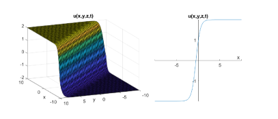
Case-1
which gives:
| (15) |
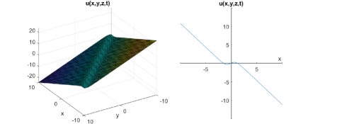
Case-2
which gives:
| (16) |
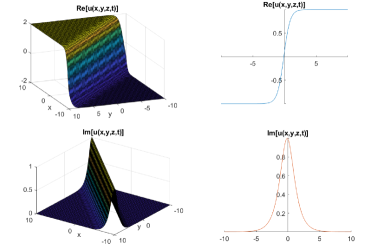
Case-3
which gives:
| (17) |
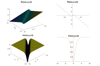
Case-4
which gives:
| (18) |
3.2 The Reaction-Diffusion Equation
We consider the following form of the reaction-diffusion equation [46],
| (19) |
where , and are constants (nonzero). The moving coordinate , where leads the Eq. (19) in an ordinary differential equation (ODE)
| (20) |
Considering homogeneous balance between and in Eq. (20) based on Eq. (9) we obtain , which implies . Now we can write Eq. (9) as
| (21) |
Using Eq. (21) into Eq. (20), and equaling all polynomials with same degree to get, we have a system of equation as below.
constant:
After solving the above system , we find the traveling wave solution to Eq. (19) in the form of (8).
Case-1
which gives:
| (22) |
Case-2
which gives:
| (23) |
Case-3
which gives:
| (24) |
4 Conclusion
In this article, we have applied the Sine-Gordon expansion method for calculating new travelling wave solutions to the potential-YTSF equation of dimension (3+1) and the reaction-diffusion equation. We have found these solutions of the equation in the trigonometric, complex and hyperbolic function forms. This method is powerful and very efficient to finding travelling wave solutions to the NLEEs. We can solve various NLEEs by this method using any symbolic software.
Abbreviations
NLEEs, SGE and ODE.
Declarations
Availability of data and material: Not applicable.
Competing interests:
The author has no any financial or non-financial conflict of interests.
Funding : There was no funding for this research.
Authors’ contributions: The Author did the research (methodology, examples and writing ) by himself and approved the final manuscript.
Acknowledgements: The author is very grateful to the editorial team and reviewers for their valuable comments and suggestions towards improving this article.
References
- [1] M. Ablowitz, D. Kaup, A. Newell, and H. Segur, “Nonlinear-evolution equations of physical significance,” Physical Review Letters, vol. 31, no. 2, pp. 125–127, 1973, https://doi.org/10.1103/PhysRevLett.31.125.
- [2] H. Brezis and T. Gallouet, “Nonlinear schrödinger evolution equations,” Nonlinear Analysis, vol. 4, no. 4, pp. 677–681, 1980, https://doi.org/10.1016/0362-546X(80)90068-1.
- [3] J. Hill and D. Hill, “High-order nonlinear evolution equations,” IMA Journal of Applied Mathematics (Institute of Mathematics and Its Applications), vol. 45, no. 3, pp. 243–265, 1990, https://doi.org/10.1093/imamat/45.3.243.
- [4] B. L. Keyfitz and M. Shearer, Nonlinear Evolution Equations That Change Type edited by Barbara L. Keyfitz, Michael Shearer., 1st ed., ser. The IMA Volumes in Mathematics and its Applications, 27. New York, NY: Springer New York : Imprint: Springer, 1990, https://doi.org/10.1007/978-1-4613-9049-7.
- [5] X. Geng, “4 new hierarchies of nonlinear evolution-equations,” Physics Letters A, vol. 147, no. 8-9, pp. 491–494, 1990, https://doi.org/10.1016/0375-9601(90)90613-S.
- [6] R. H. Enns, B. L. Jones, R. M. Miura, and S. S. Rangnekar, Nonlinear Phenomena in Physics and Biology edited by Richard H. Enns, Billy L. Jones, Robert M. Miura, Sadanand S. Rangnekar., ser. NATO Advanced Study Institutes Series, Series B: Physics, 75. Boston, MA: Springer New York, 1981, https://doi.org/10.1007/978-1-4684-4106-2.
- [7] R. K. Dodd, Solitons and nonlinear wave equations / R.K. Dodd … [et al.]. London ; New York: Academic Press, 1982, https://doi.org/10.1137/1026058.
- [8] Y. Zhou, M. Wang, and Y. Wang, “Periodic wave solutions to a coupled KdV equations with variable coefficients,” Physics Letters A, vol. 308, no. 1, pp. 31–36, 2003, https://doi.org/10.1016/S0375-9601(02)01775-9.
- [9] M. J. Ablowitz and H. Segur, Solitons and the inverse scattering transform / Mark J. Ablowitz and Harvey Segur., ser. SIAM studies in applied mathematics ; 4. Philadelphia: SIAM, 1981, https://doi.org/10.1137/1.9781611970883.
- [10] R. Hirota, A. Nagai, J. Nimmo, and C. Gilson, The Direct Method in Soliton Theory. Cambridge University Press, 2004, https://doi.org/10.1017/CBO9780511543043.
- [11] W. Malfliet, “Solitary wave solutions on nonlinear wave equations,” American Journal of Physics, vol. 60, no. 7, p. 650, 1992, https://doi.org/10.1119/1.17120.
- [12] M. Wang, X. Li, and J. Zhang, “The ( )-expansion method and travelling wave solutions of nonlinear evolution equations in mathematical physics,” Physics Letters A, vol. 372, no. 4, pp. 417–423, 2008, https://doi.org/10.1016/j.physleta.2007.07.051.
- [13] A. Khater, W. Malfliet, D. Callebaut, and E. Kamel, “The tanh method, a simple transformation and exact analytical solutions for nonlinear reaction–diffusion equations,” Chaos, Solitons and Fractals, vol. 14, no. 3, pp. 513–522, 2002, https://doi.org/10.1016/S0960-0779(01)00247-8.
- [14] A. M. Wazwaz, “The tanh method: solitons and periodic solutions for the dodd–bullough–mikhailov and the tzitzeica–dodd–bullough equations,” Chaos, Solitons and Fractals, vol. 25, no. 1, pp. 55–63, 2005, https://doi.org/10.1016/j.chaos.2004.09.122.
- [15] ——, “Abundant solitons solutions for several forms of the fifth-order KdV equation by using the tanh method,” Applied Mathematics and Computation, vol. 182, no. 1, pp. 283–300, 2006, https://doi.org/10.1016/j.amc.2006.02.047.
- [16] Y.-T. Gao and B. Tian, “Generalized tanh method with symbolic computation and generalized shallow water wave equation,” Computers and Mathematics with Applications, vol. 33, no. 4, pp. 115–118, 1997, https://doi.org/10.1016/S0898-1221(97)00011-4.
- [17] W.-Q. Hu, Y.-T. Gao, S.-L. Jia, Q.-M. Huang, and Z.-Z. Lan, “Periodic wave, breather wave and travelling wave solutions of a (2 + 1)-dimensional b-type kadomtsev-petviashvili equation in fluids or plasmas,” The European Physical Journal Plus, vol. 131, no. 11, pp. 1–19, 2016, https://doi.org/10.1140/epjp/i2016-16390-1.
- [18] E. Yusufoğlu and A. Bekir, “Symbolic computation and new families of exact travelling solutions for the kawahara and modified kawahara equations,” Computers and Mathematics with Applications, vol. 55, no. 6, pp. 1113–1121, 2008, https://doi.org/10.1016/j.camwa.2007.06.018.
- [19] J. Manafian, “Applications of he’s semi-inverse method, item and ggm to the davey-stewartson equation,” The European Physical Journal Plus, vol. 132, no. 4, pp. 1–26, 2017, https://doi.org/10.1140/epjp/i2017-11463-3.
- [20] M. I. Ismailov, “Integration of nonlinear system of four waves with two velocities in (2 + 1) dimensions by the inverse scattering transform method,” Journal of Mathematical Physics, vol. 52, no. 3, 2011, https://doi.org/10.1063/1.3560476.
- [21] H. Baskonus, H. Bulut, and T. Sulaiman, “Investigation of various travelling wave solutions to the extended (2+1)-dimensional quantum zk equation,” The European Physical Journal Plus, vol. 132, no. 11, pp. 1–8, 2017, https://doi.org/10.1140/epjp/i2017-11778-y.
- [22] S. El-Wakil and M. Abdou, “New explicit and exact traveling wave solutions for two nonlinear evolution equations,” Nonlinear Dynamics, vol. 51, no. 4, pp. 585–594, 2008, https://doi.org/10.1007/s11071-007-9247-9.
- [23] M. El-Borai, H. El-Owaidy, H. Ahmed, and A. Arnous, “Exact and soliton solutions to nonlinear transmission line model,” Nonlinear Dynamics, vol. 87, no. 2, pp. 767–773, 2017, https://doi.org/10.1007/s11071-016-3074-9.
- [24] A. M. Wazwaz and S. A. El-Tantawy, “New (3 + 1)-dimensional equations of burgers type and sharma–tasso–olver type: multiple-soliton solutions.(report),” Nonlinear Dynamics, vol. 87, no. 4, pp. 2457–2461, 2017, https://doi.org/10.1007/s11071-016-3203-5.
- [25] M. Darvishi, S. Arbabi, M. Najafi, and A. Wazwaz, “Traveling wave solutions of a (2+1)-dimensional zakharov-like equation by the first integral method and the tanh method,” Optik - International Journal for Light and Electron Optics, vol. 127, no. 16, pp. 6312–6321, 2016, https://doi.org/10.1016/j.ijleo.2016.04.033.
- [26] K. Hosseini, Z. Ayati, and R. Ansari, “New exact traveling wave solutions of the tzitzéica type equations using a novel exponential rational function method,” Optik - International Journal for Light and Electron Optics, vol. 148, pp. 85–89, 2017, https://doi.org/10.1016/j.ijleo.2017.08.030.
- [27] E. Zayed, A. Al-Nowehy, and M. Elshater, “Solitons and other solutions to nonlinear schrodinger equation with fourth-order dispersion and dual power law nonlinearity using several different techniques,” European Physical Journal Plus, vol. 132, no. 6, 2017, https://doi.org/10.1140/epjp/i2017-11527-4.
- [28] A. R. Seadawy, D. Lu, and M. M. Khater, “Bifurcations of solitary wave solutions for the three dimensional zakharov–kuznetsov–burgers equation and boussinesq equation with dual dispersion,” Optik, vol. 143, pp. 104–114, 2017, https://doi.org/10.1016/j.ijleo.2017.06.020.
- [29] M. Boudoue Hubert, N. Kudryashov, M. Justin, S. Abbagari, G. Betchewe, and S. Doka, “Exact traveling soliton solutions for the generalized benjamin-bona-mahony equation,” The European Physical Journal Plus, vol. 133, no. 3, pp. 1–6, 2018, https://doi.org/10.1140/epjp/i2018-11937-8.
- [30] O. Ilhan, T. Sulaiman, H. Bulut, and H. Baskonus, “On the new wave solutions to a nonlinear model arising in plasma physics,” The European Physical Journal Plus, vol. 133, no. 1, pp. 1–6, 2018, https://doi.org/10.1140/epjp/i2018-11858-6.
- [31] Y. Amadou, G. Betchewe, M. Douvagai, S. Y. Justin, K. T. Doka, and K. T. Crepin, “Discrete exact solutions for the double-well potential model through the discrete tanh method,” The European Physical Journal Plus, vol. 130, no. 1, pp. 1–10, 2015.
- [32] B. Ghanbari and D. Baleanu, “A novel technique to construct exact solutions for nonlinear partial differential equations,” The European Physical Journal Plus, vol. 134, no. 10, pp. 1–21, 2019, https://doi.org/10.1140/epjp/i2019-13037-9.
- [33] C. Yan, “A simple transformation for nonlinear waves,” Physics Letters A, vol. 224, no. 1-2, pp. 77–84, 1996, https://doi.org/10.1016/S0375-9601(96)00770-0.
- [34] G. Yel, H. Baskonus, and H. Bulut, “Novel archetypes of new coupled konno–oono equation by using sine–gordon expansion method,” Optical and Quantum Electronics, vol. 49, no. 9, pp. 1–10, 2017, https://doi.org/10.1007/s11082-017-1127-z.
- [35] D. Kumar, K. Hosseini, and F. Samadani, “The sine-gordon expansion method to look for the traveling wave solutions of the tzitzéica type equations in nonlinear optics,” Optik - International Journal for Light and Electron Optics, vol. 149, pp. 439–446, 2017, https://doi.org/10.1016/j.ijleo.2017.09.066.
- [36] A. Korkmaz, O. E. Hepson, K. Hosseini, H. Rezazadeh, and M. Eslami, “Sine-gordon expansion method for exact solutions to conformable time fractional equations in rlw-class,” Journal of King Saud University - Science, vol. 32, no. 1, pp. 567–574, 2020, https://doi.org/10.1016/j.jksus.2018.08.013.
- [37] H. Bulut, T. Sulaiman, H. Baskonus, and T. Yazgan, “Novel hyperbolic behaviors to some important models arising in quantum science,” Optical and Quantum Electronics, vol. 49, no. 11, pp. 1–17, 2017, https://doi.org/10.1007/s11082-017-1181-.
- [38] J. Rubinstein, “Sine-gordon equation,” Journal of Mathematical Physics, vol. 11, no. 1, pp. 258–266, 1970, https://doi.org/10.1063/1.1665057.
- [39] A. Barone, F. Esposito, C. Magee, and A. Scott, “Theory and applications of the sine-gordon equation,” La Rivista del Nuovo Cimento, vol. 1, no. 2, pp. 227–267, 1971, https://doi.org/10.1007/BF02820622.
- [40] S.-J. Yu, “n soliton solutions to the bogoyavlenskii-schiff equation and a quest for the soliton solution in dimensions,” Journal of Physics A: Mathematical and General, vol. 31, no. 14, pp. 3337–3347, 1998, https://doi.org/10.1088/0305-4470/31/14/018.
- [41] E. M. E. Zayed, “New traveling wave solutions for higher dimensional nonlinear evolution equations using a generalized -expansion method,” Journal of Physics A: Mathematical and Theoretical, vol. 42, no. 19, p. 195202, apr 2009, https://doi.org/10.1088
- [42] A. M. Wazwaz, “New solutions of distinct physical structures to high-dimensional nonlinear evolution equations,” Applied Mathematics and Computation, vol. 196, no. 1, pp. 363–370, 2008, https://doi.org/10.1016/j.amc.2007.06.002.
- [43] Z. Yan, “New families of nontravelling wave solutions to a new (3+1)-dimensional potential-ytsf equation,” Physics Letters A, vol. 318, no. 1-2, pp. 78–83, 2003, https://doi.org/10.1016/j.physleta.2003.08.073.
- [44] C.-L. Bai and H. Zhao, “Generalized method to construct the solitonic solutions to ( 3 + 1 ) -dimensional nonlinear equation,” Physics Letters A, vol. 354, no. 5, pp. 428–436, 2006, https://doi.org/10.1016/j.physleta.2006.01.084.
- [45] Z. Li-Hua, “New exact solutions and conservation laws to (3+1)-dimensional potential-ytsf equation,” Communications in Theoretical Physics, vol. 45, no. 3, pp. 487–492, 2006, https://doi.org/10.1088/0253-6102/45/3/022.
- [46] E. Zayed and K. Gepreel, “The -expansion method for finding traveling wave solutions of nonlinear partial differential equations in mathematical physics,” Journal Of Mathematical Physics, vol. 50, no. 1, 2009, https://doi.org/10.1063/1.3033750.