A Novel Algorithm for Joint Bit and Power Loading for OFDM Systems with Unknown Interference

An OFDM system decomposes the signal bandwidth into a set of $N$ orthogonal narrowband subcarriers of equal bandwidth. Each subcarrier $i$ transmits $b_{i}$ bits using power $\mathcal{P}_{i}$, $i=1,...,N$. An unknown interference is assumed to affect the OFDM signal, with a Gaussian distribution with zero mean and variance $\sigma^{2}_{u,i}$ per subcarrier $i$ [16, 17, 18, 19]; according to the central limit theorem [20], such an assumption is valid assuming the interference comes from several independent sources. A delay- and error-free feedback channel is assumed to exist between the transmitter and receiver for reporting channel state information.

In order to minimize the total transmit power and maximize the throughput subject to a BER constraint, the optimization problem is formulated as

where $\mathcal{P}_{T}$ and $b_{T}$ are the total transmit power and throughput, respectively, and $\textup{BER}_{i}$ and $\textup{BER}_{th,i}$ are the BER and threshold value of BER per subcarrier $i$, $i$ = 1, …, $N$, respectively. An approximate expression for the BER per subcarrier $i$ in the case of $M$-ary QAM is given by¹¹1This expression is tight within 1 dB for BER $\leq$ $10^{-3}$ [21]. [12, 21]

where $\mathcal{H}_{i}$ is the channel gain of subcarrier $i$ and $\sigma^{2}_{n}$ is the variance of the additive white Gaussian noise (AWGN).

The multi-objective optimization function in (1) can be rewritten as a linear combination of multiple objective function as follows

where $\alpha$ ($0<\alpha<1$) is a constant whose value indicates the relative importance of one objective function relative to the other, $\mathcal{C}_{i}=\>\frac{\left|\mathcal{H}_{i}\right|^{2}}{\sigma^{2}_{n}+\sigma^{2}_{u,i}}$ is the channel-to-interference-plus-noise ratio for subcarrier $i$, and $\textbf{{P}}=[\mathcal{P}_{1},...,\mathcal{P}_{N}]^{T}$ and $\textbf{{b}}=[b_{1},...,b_{N}]^{T}$ are the N-dimensional power and bit distribution vectors, respectively, with $[.]^{T}$ denoting the transpose operation.

The problem in (3) can be solved by applying the method of Lagrange multipliers. Accordingly, the inequality constraints are transformed to equality constraints by adding non-negative slack variables, $\mathcal{Y}_{i}^{2}$, $i$ = 1, …, $N$ [22]. Hence, the constraints are rewritten as

and the Lagrange function $\mathcal{L}$ is then expressed as

where $\mathbf{\Lambda}=[\lambda_{1},...,\lambda_{N}]^{T}$ and $\textbf{{Y}}=[\mathcal{Y}_{1}^{2},...,\mathcal{Y}_{N}^{2}]^{T}$ are the vectors of Lagrange multipliers and slack variables, respectively. A stationary point can be found when $\nabla\mathcal{L}(\textbf{{P}},\textbf{{b}},\textbf{{Y}},\mathbf{\Lambda})=0$ (where $\nabla$ denotes the gradient), which yields

It can be seen that (6) to (9) represent $4N$ equations in the $4N$ unknown components of the vectors $\textbf{{P}},\textbf{{b}},\textbf{{Y}}$, and $\mathbf{\Lambda}$. By solving (6) to (9), one obtains the solution $\textbf{{P}}^{*},\textbf{{b}}^{*}$, the slack variable vector $\textbf{{Y}}^{*}$, and the Lagrange multiplier vector $\mathbf{\Lambda}^{*}$. Equation (9) implies that either $\lambda_{i}$ = 0 or $\mathcal{Y}_{i}$ = 0; hence, two possible solutions exist, and we are going to investigate each case independently.

— Case 1 ($\mathcal{Y}_{i}=0$): From (6) and (7), we can relate $\mathcal{P}_{i}$ and $b_{i}$ as

with $\mathcal{P}_{i}\geq 0$ if and only if $b_{i}\geq 0$. By substituting (10) into (8), one obtains the solution

Consequently, from (10) one gets

Since (2) is valid for $M$-ary QAM, $b_{i}$ should be greater than 2. From (11), to have $b_{i}\geq 2$, the channel-to-noise ratio per subcarrier, $\mathcal{C}_{i}$, must satisfy the condition

— Case 2 ($\lambda_{i}=0$): By following a similar procedure as in Case 1, one can show that $\nabla\mathcal{L}(\textbf{{P}},\textbf{{b}},\textbf{{Y}},\mathbf{\Lambda})=0$ results in an underdetermined system of $N$ equations in $4N$ unknowns, and, hence, no unique solution can be reached.

The obtained solution represents a minimum of $\mathcal{F}(\textbf{{P}},\textbf{{b}})$ if the Karush-Kuhn-Tucker conditions are satisfied [23]. Given that our stationary point ($b_{i}^{*}$, $\mathcal{P}_{i}^{*}$) in (11) and (12) exists at $\mathcal{Y}_{i}=0$, $i$ = 1, …, $N$, the Karush-Kuhn-Tucker conditions can be written as

$i$, $j$ = 1, …, $N$. One can easily prove that these conditions are fulfilled, as follows.

Proof of (14)-(16): From (6), one finds

which is positive for all values of $j$, and hence it satisfies (16). Furthermore, by substituting (11), (12), and (17) into (14) and (15), one can easily verify that the rest of the Karush-Kuhn-Tucker conditions are satisfied, and, thus, the solution ($\textbf{{b}}^{*},\textbf{{P}}^{*}$) represents an optimum point. $\blacksquare$

The idea behind the proposed algorithm is to check the channel-to-interference-plus-noise ratio per subcarrier, $\mathcal{C}_{i}$, against the condition in (13). If this is fulfilled, the optimal bit and power is given by (11) and (12), respectively; otherwise, the corresponding subcarrier is nulled. The final bit and power allocation is reached after rounding the non-integer number of bits obtained from (11) to the nearest integer and recalculating the allocated power according to (2). The proposed algorithm can be formally stated as follows.

An OFDM system with a total of $N$ = 128 subcarriers is considered. Without loss of generality, the unknown interference is assumed to affect $N_{u}$ subcarriers, $N_{u}$ = 40, with exponentially distributed variance across the affected subcarriers²²2Such distribution is chosen to approximate the effect of narrowband interference signals on the OFDM subcarriers noticed from simulations; however other distributions can be straightforwardly applied., i.e., $\sigma^{2}_{u,i}=e^{-\beta x}$, $\beta=-0.25$, $x$ = 0,…,$N_{u}-1$. For simplicity, the BER constraint per subcarrier, $\textup{BER}_{th,i}$, is assumed to be the same for all subcarriers and set to $10^{-4}$. The channel impulse response $h(n)$ of length $N_{ch}$ is modeled as independent complex Gaussian random variables with zero mean and exponential power delay profile [24]

where $\sigma_{h}^{2}$ is a constant chosen such that the average energy per subcarrier is normalized to unity, i.e., $\mathbb{E}\{\left|\mathcal{H}_{i}\right|^{2}\}$ = 1, and $\Xi$ represents the decay factor. Representative results are presented in this section and were obtained by repeating Monte Carlo trials for $10^{5}$ channel realizations with a channel length $N_{ch}=5$ taps and decay factor $\Xi=\frac{1}{5}$.

Fig. 1 illustrates the allocated bits and power computed using (11) and (12), respectively, for an example channel realization with $\sigma_{n}^{2}=10^{-3}$ $\mu W$ and $\alpha$ = 0.5. It can be seen from the plots in Fig. 1 that when the channel-to-interference-plus-noise ratio per subcarrier, $\mathcal{C}_{i}$, exceeds the value in (13), the number of bits and power allocated per subcarrier are non-zero. As expected, (11) yields a non-integer number of allocated bits per subcarrier, which is not suitable for practical implementations. This value is rounded to the nearest integer, as shown in Fig. 1 (b), and the modified value of the allocated power per subcarrier to maintain the same $\textup{BER}_{th,i}$ is determined using (2).

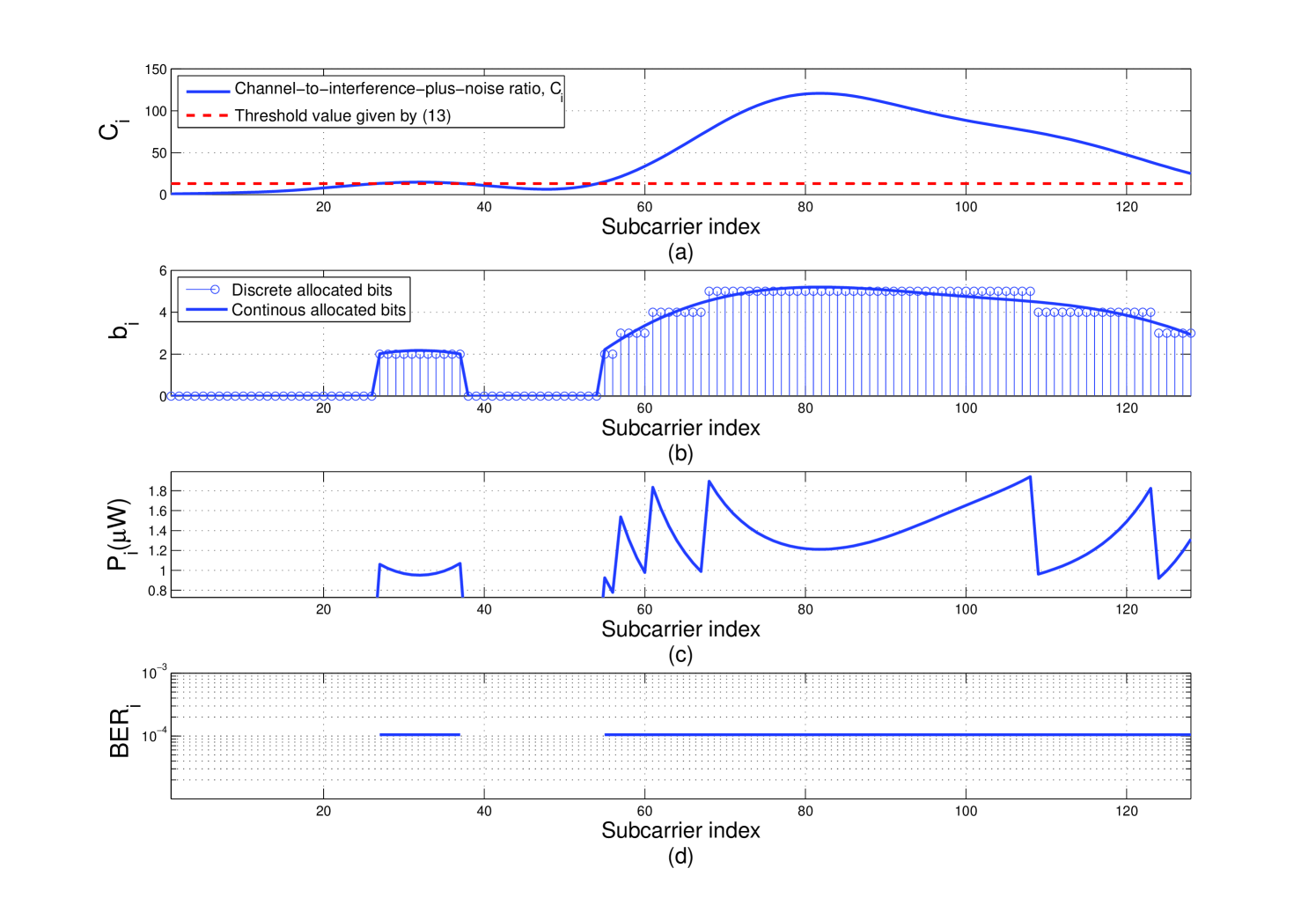
Fig. 2 depicts the average throughput and average transmit power when $\alpha$ = 0.5 as a function of average SNR, for different average SIR values³³3The average SNR is calculated by averaging the instantaneous SNR values per subcarrier over the total number of subcarriers and the total number of channel realizations, respectively. Moreover, the average SIR is calculated by averaging the instantaneous SIR values per subcarrier over the total number of affected subcarriers and the total number of channel realizations, respectively.. For an average SIR $\rightarrow\infty$, i.e., no interference, and average SNR $\leq$ 24 dB, one finds that both the average throughput and the average transmit power increase as the average SNR increases, while for an average SNR $\geq$ 24 dB, the transmit power saturates while the throughput continues to increase. This observation can be explained as follows. For lower values of average SNR, the corresponding values of $\mathcal{C}_{i}$ result in the nulling of many subcarriers in (13). By increasing the average SNR, the number of used subcarriers increases, resulting in a noticeable increase in the throughput and power. Apparently, for SNR $\geq$ 24 dB, all subcarriers are used and our proposed algorithm essentially minimizes the average transmit power by keeping it constant, while increasing the average throughput. On the other hand, reducing the average SIR, increases the effect of the interference on the OFDM system and more subcarriers are nulled, hence, both the average throughput and transmit power decrease as in Fig. 2. For SIR $\rightarrow-\infty$, i.e., very strong interference, all $N_{u}$ affected subcarriers are nulled and both the average throughput and transmit power are affected accordingly. Note that this provides a lower performance bound for a given number of affected subcarriers, $N_{u}$.

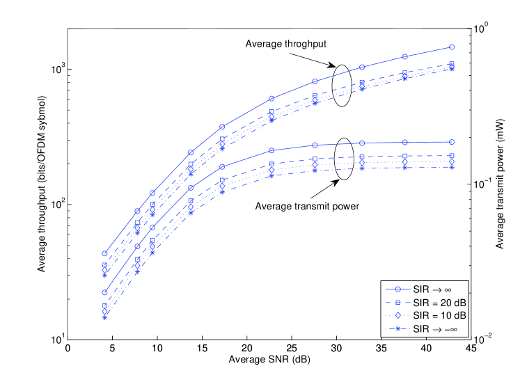
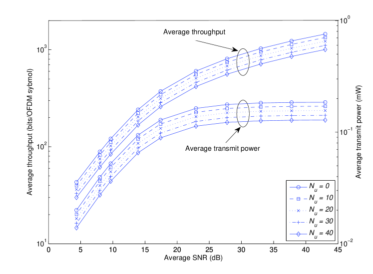
Fig. 3 shows the average throughput and average transmit power as a function of average SNR, for diverse $N_{u}$ and $\alpha$ = 0.5. For $N_{u}$ = 0, i.e., no interference, the average throughput increases as the average SNR increases, while, the average transmit power increases for lower values of average SNR and saturates for higher values as discussed earlier. As $N_{u}$ increases, more subcarriers are affected by the interference, and hence, both the average throughput and average transmit power decreases.

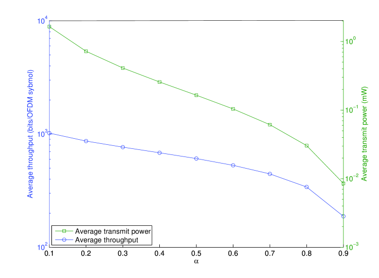
In Fig. 4, the average throughput and average transmit power are plotted as a function of the weighting factor $\alpha$, for $\sigma_{n}^{2}=10^{-3}$ $\mu$W and $\sigma_{u,i}^{2}$ = 0 (no interference). By increasing $\alpha$, more weight is given in our problem formulation to minimizing the transmit power over maximizing the throughput. In this case, the corresponding reduction in the minimum transmit power is accompanied by a reduction in the maximum throughput.

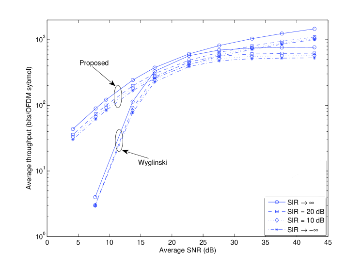
In Fig. 5, the throughput achieved by the proposed algorithm is compared with that obtained by Wyglinski’s algorithm presented in [1] for the same operating conditions. To make a fair comparison, the uniform power allocation used by the allocation scheme in [7] is computed by dividing the average transmit power allocated by our algorithm by the total number of subcarriers. As can be seen in Fig. 5, the proposed algorithm provides a significantly higher throughput than the scheme in [1] for low average SNR values. This result demonstrates that optimal allocation of transmit power is crucial for low power budgets. Furthermore, for increasing average SNR values, the average transmit power is constant as seen in Fig. 2 for values $\geq$ 24 dB, which in turn results in a saturating throughput for Wyglinski’s algorithm. In contrast, the proposed algorithm provides an increasing throughput for the same range of SNR values. As expected, increasing the effect of the interference, i.e., decreasing SIR, reduces the average throughput.

The improved performance of the proposed joint bit and power allocation algorithm does not come at the cost of additional complexity. The proposed algorithm is non-iterative with a worst case computational complexity of $\mathcal{O(N)}$, while Wyglinski’s algorithm is iterative with a worst case computational complexity of $\mathcal{O}(\mathcal{N}^{2})$.

References

- [1] A. Wyglinski, F. Labeau, and P. Kabal, “Bit loading with BER-constraint for multicarrier systems,” IEEE Trans. Wireless Commun., vol. 4, no. 4, pp. 1383–1387, Jul. 2005.
- [2] D. Popescu and P. Yaddanapudi, “Narrowband interference avoidance in OFDM-based UWB communication systems,” IEEE Trans. Commun., vol. 55, no. 9, pp. 1667–1673, Sep. 2007.
- [3] X. Wang, H. Li, and H. Lin, “A new adaptive OFDM system with precoded cyclic prefix for dynamic cognitive radio communications,” IEEE J. Sel. Areas Commun., vol. 29, no. 2, pp. 431–442, Feb. 2011.
- [4] K. Fazel and S. Kaiser, Multi-carrier and Spread Spectrum Systems: from OFDM and MC-CDMA to LTE and WiMAX. John Wiley & Sons Inc, 2008.
- [5] D. Hughes-Hartogs, “Ensemble modem structure for imperfect transmission media,” Mar. 15 1988, US Patent 4,731,816.
- [6] J. Campello, “Optimal discrete bit loading for multicarrier modulation systems,” in Proc. IEEE Symp. Information Theory, 1998, p. 193.
- [7] H. Levin, “A complete and optimal data allocation method for practical discrete multitone systems,” in Proc. IEEE Global Telecommunications Conference (GLOBECOM), 2001, pp. 369–374.
- [8] B. Fox, “Discrete optimization via marginal analysis,” Management Science, vol. 13, no. 3, pp. 210–216, Nov. 1966.
- [9] Z. Song, K. Zhang, and Y. Guan, “Joint bit-loading and power-allocation for OFDM systems based on statistical frequency-domain fading model,” in Proc. IEEE Vehicular Technology Conference (VTC)-Fall, Sep. 2002, pp. 724–728.
- [10] R. Sonalkar and R. Shively, “An efficient bit-loading algorithm for DMT applications,” IEEE Commun. Lett., vol. 4, no. 3, pp. 80–82, Mar. 2000.
- [11] N. Papandreou and T. Antonakopoulos, “A new computationally efficient discrete bit-loading algorithm for DMT applications,” IEEE Trans. Commun., vol. 53, no. 5, pp. 785–789, May 2005.
- [12] K. Liu, B. Tang, and Y. Liu, “Adaptive power loading based on unequal-BER strategy for OFDM systems,” IEEE Commun. Lett., vol. 13, no. 7, pp. 474–476, Jul. 2009.
- [13] L. Goldfeld, V. Lyandres, and D. Wulich, “Minimum BER power loading for OFDM in fading channel,” IEEE Trans. Commun., vol. 50, no. 11, pp. 1729–1733, Nov. 2002.
- [14] B. Krongold, K. Ramchandran, and D. Jones, “Computationally efficient optimal power allocation algorithms for multicarrier communication systems,” IEEE Trans. Commun., vol. 48, no. 1, pp. 23–27, Jan. 2000.
- [15] T. Cover and J. Thomas, Elements of Information Theory. Wiley, New York NY, 2004.
- [16] G. Bansal, M. Hossain, and V. Bhargava, “Optimal and suboptimal power allocation schemes for OFDM-based cognitive radio systems,” IEEE Trans. Wireless Commun., vol. 7, no. 11, pp. 4710–4718, Nov. 2008.
- [17] C. Zhao and K. Kwak, “Power/bit loading in OFDM-based cognitive networks with comprehensive interference considerations: The single-SU case,” IEEE Trans. Veh. Technol., vol. 59, no. 4, pp. 1910–1922, May 2010.
- [18] L. Sanguinetti, M. Morelli, and H. Poor, “Frame detection and timing acquisition for OFDM transmissions with unknown interference,” IEEE Trans. Wireless Commun., vol. 9, no. 3, pp. 1226–1236, Mar. 2010.
- [19] Z. Wu and C. Nassar, “Narrowband interference rejection in OFDM via carrier interferometry spreading codes,” IEEE Trans. Wireless Commun., vol. 4, no. 4, pp. 1491–1505, Jul. 2005.
- [20] A. Papoulis, S. Pillai, and S. Unnikrishna, Probability, Random Variables, and Stochastic Processes. McGraw-hill, New York NY, 1965.
- [21] S. Chung and A. Goldsmith, “Degrees of freedom in adaptive modulation: a unified view,” IEEE Trans. Commun., vol. 49, no. 9, pp. 1561–1571, Sep. 2001.
- [22] I. Griva, S. Nash, and A. Sofer, Linear and Nonlinear Optimization. Society for Industrial Mathematics, 2009.
- [23] H. Kuhn and A. Tucker, “Nonlinear programming,” in Proceedings of the Second Berkeley Symposium on Mathematical Statistics and Probability, 1951, pp. 481–492.
- [24] M. Marey and H. Steendam, “Analysis of the narrowband interference effect on OFDM timing synchronization,” IEEE Trans. Signal Process., vol. 55, no. 9, pp. 4558–4566, Sep. 2007.