A Novel Reversible Data Hiding Scheme Based on Asymmetric Numeral Systems
Abstract
Reversible data hiding (RDH) has been extensively studied in the field of information security. In our previous work [1], an explicit implementation approaching the rate-distortion bound of RDH has been proposed. However, there are two challenges left in our previous method. Firstly, this method suffers from computing precision problem due to the use of arithmetic coding, which may cause the further embedding impossible. Secondly, it had to transmit the probability distribution of the host signals during the embedding/extraction process, yielding quite additional overhead and application limitations. In this paper, we first propose an RDH scheme that employs our recent asymmetric numeral systems (ANS) variant as the underlying coding framework to avoid the computing precision problem. Then, we give a dynamic implementation that does not require transmitting the host distribution in advance. The simulation results show that the proposed static method provides slightly higher peak signal-to-noise ratio (PSNR) values than our previous work, and larger embedding capacity than some state-of-the-art methods on gray-scale images. In addition, the proposed dynamic method totally saves the explicit transmission of the host distribution and achieve data embedding at the cost of a small image quality loss.
Index Terms:
Reversible data hiding, Gray-scale signals, Embedding capacity, PSNR, Asymmetrical numeral systems.I Introduction
Reversible data hiding (RDH) aims at secure transmission of secret data through communication media. This is achieved through embedding of secret data into the host media, and it has the property that the receiver can losslessly reconstruct the host media and secret data from the received steganographic (abbreviated as stego) media. A media used to embed data is defined as the host media, including image, text file, audio, video and multimedia, and the media that has embedded secret data is called the stego media. RDH is widely adopted in medical imagery [2], image authentication [3] and law forensics, where the host media is so precious that cannot be damaged.
In the past two decades, many RDH works have emerged and they are categorized mainly into plain domain and encrypted domain. Plain domain approaches of RDH are designed to achieve high embedding capacity and low distortion without any protection of the host media, where embedding capacity is defined as a ratio between the number of secret data bits and host signals. The purpose of RDH in encrypted domain is to embed additional data into the encrypted media without revealing the plaintext data. This paper focuses on the RDH methods in the plain domain. Popular plain domain works roughly categorized as i) difference expansion (DE) [4, 5, 6, 7], ii) histogram shifting (HS) [8, 9, 10, 11] and iii) lossless compression [12, 13, 14, 15]. In the DE-based RDH methods, the differences of each pixel group are expanded, e.g., multiplied by , so that the lowest significant bits (LSB) of the differences are all zero and can be used to embed data. In [5], Tian introduced the first difference expansion method based on integer transform, but it suffers from low embedding capacity and its overhead cost was almost double the amount of hiding data. To remedy this problem, A.M. Alattar [16] gave a generalized integer transform, and pixel block of arbitrary size was considered instead of pixel pairs, to improve the embedding capacity. However, this method is applicable only for color images.
Histogram is a graphical representation of data points. The maximum and minimum number of occurrence of elements in the set of data points are called peak point and zero point, respectively. Histogram shifting (HS) is an effective method for RDH, it improves the embedding capacity by enlarging the peak pixels. When images are selected as the host media, the peak signal-to-noise ratio (PSNR) is often used as a metric to measure the performance of an RDH scheme, and the higher the PSNR, the better the stego image quality. In 2006, Ni et al. [17] chosen the bins with the highest frequencies in the histogram to embed the secret bits. In this method, each pixel value is modified at most by 1, thus the PSNR of stego image is guaranteed. Yet, this approach suffers from the issues of multiple zero points, which requires the storage for the coordinate of zero points. In [18], Fallahpour et al. improved the embedding capacity of Ni et al.’s method by applying HS on blocks instead of the whole image. However, this technique bears zero and peak point information that needs to be transmitted to the receiver for data retrieval. Tai et al. [19] presented an RDH scheme based on histogram modification. In this method, the binary tree structure was exploited to solve the issue of multiple pairs of peak points for communication. But, its pure embedding capacity unexpectedly decreases with increasing tree level and the overhead information increases as well. In [20], Ou et al. proposed an RDH method based on multiple histogram modification to achieve high embedding capacity, by using multiple pairs of bins for every prediction error histogram. However, the location map as overhead information is necessary to preserve reversibility, and it can be large even after compression.
The lossless compression algorithm is extensively explored in RDH technique. The main idea is to save space for hiding additional data by performing lossless compression on the host media. Celik [12] introduced a generalization least significant bit (G-LSB) method to enhance the compression effectiveness by using arithmetic coding. In this method, the embedding capacity was enhanced as higher level pixel was considered. However, when the higher level was used, the distortion of host media also increased. In [21], Manikandan employed run-length encoding and a modified Elias gamma encoding to embed some additional bits during the encoding process itself. Moreover, one natural problem is what is the upper limit of the embedding capacity for a given host media and distortion constraint. This problem was solved by Kalker et al. [22] for independent and identically distributed (i.i.d.) host sequence. In [22], Kalker and Willems formulated the rate-distortion function, i.e., the upper bound of the embedding rate under a given distortion constraint as follows:
| (1) |
where and denote the random variables of host media and stego media respectively, and is the Shannon entropy of a discrete random variable. The entropy is maximized over all transition probabilities satisfying the distortion constraint
| (2) |
where is the probability mass function (pmf) of host sequence , and the distortion metric is usually defined as the square error distortion, i.e., . Therefore, to evaluate the embedding capacity of an RDH scheme, the optimal transition probability (OTP) needs to be calculated. For some specific distortion metrics , such as the square error distortion or L1-Norm , it has been proved that the OTP has a Non-Crossing-Edges (NCE) property [23]. Based on the NCE property, our previous work [1] found that the optimal solution on can be derived from the analysis of pmfs and . Because is available from the given host sequence , this means that the encoder and decoder only need to calculate the for the distortion metric that satisfies the NCE property.
In our previous work [1], we proposed a backward and forward iterative (BFI) algorithm to estimate the optimal pmf . Also, we gave an arithmetic coding [24]-based scheme that can approach the rate-distortion bound (1). After that, Hu et al. [25] introduced a fast algorithm to estimate the in our previous work. However, there are still two challenges unresolved in our previous work [1]. Firstly, we adopted arithmetic coding as the underlying coding framework in [1] to embed a message in the i.i.d. host sequence. In the arithmetic coding, there is a limit to the precision of the number that can be encoded, which constrains the number of symbols to encode within a codeword. As a result, our previous work [1] suffers from the computing precision problem in some special cases. For example, if the coding interval in the arithmetic coding is narrowed to zero, then further data embedding is impossible. Secondly, both the embedding and extraction processes of methods [1], [25] require transmitting the host pmf as parameters (for the purpose of estimating ), which costs quite additional overhead, and the overhead size is proportional to the alphabet size. This is usually unacceptable for extremely memory-constrained scenarios, and it has certain limitations in practical applications.
To fully address the above two challenges left in our previous work [1], we first propose a code construction scheme that employs our recent asymmetric numeral systems (ANS) variant [26]. ANS [27, 28, 29, 30] is a family of entropy coding introduced by Jarek Duda in 2009. It has been popular and incorporated into many compressors, including Facebook Zstandard, Apple LZFSE and Google Draco 3D, because it provides the compression ratio of arithmetic coding with a processing speed similar to that of Huffman coding [31]. To the best of our knowledge, this paper is the first that employs ANS coding for RDH technique. More importantly, unlike arithmetic coding, ANS coding is not subject to the computing precision. Therefore, by using ANS coding as the underlying coding framework, our proposal can avoid the precision problem that may occur in our previous work [1]. Second, we give a dynamic embedding/extraction implementation that does not require to explicitly transmit the host pmf, thus saving additional overhead costs.
This paper considers the host media composed of i.i.d. gray-scale samples. The contributions of this paper are summarized as follows.
-
1.
A code construction scheme that employs our recent ANS variant is proposed to address the computing precision problem in our previous work [1]. To the best of our knowledge, this paper is the first that employs ANS coding for RDH technique.
-
2.
A dynamic implementation is given that does not require prior transmission of the host pmf during embedding and extraction.
-
3.
The simulations are given.
-
(a)
For the host sequences drawn from discrete normal distribution: the proposed static method provides similar embedding performance to our previous work; the proposed dynamic implementation saves the additional overhead of explicitly transmitting the host pmf at the cost of a slight embedding distortion.
-
(b)
For the gray-scale images: the proposed static method provides slightly higher PSNR values than our previous work and larger embedding rates than some state-of-the-art RDH methods; the proposed dynamic method employs predicted pmf instead of true pmf to save additional overhead and produces a small image quality loss.
-
(a)
The rest of this paper is organized as follows. Section II lists the notations and related works. Section III introduces the proposed method to achieve the rate-distortion bound. In Section IV, we give a dynamic embedding/extraction implementation without the need to transmit the host pmf. Section V shows the simulation results and Section VI concludes this work.
II Preliminaries
II-A Notations
Throughout this paper, the host sequence is composed of i.i.d. samples drawn from the probability mass function (pmf) , where the set is an alphabet of size . Let denote the cumulative pmf of . It is noted that we have and . Let denote the number of occurrences of signal in the sequence , and is the cumulative frequency of signal , where by default. The entropy function of a discrete random variable is defined as . The random variable represents a message uniformly distributed in . This paper considers embedding binary secret data into gray-scale signals, so we have and .
Given a binary stream , we construct a LIFO (Last In First Out) stack accordingly. The operation
pops bits from the bottommost position in the stack that contains , and these bits form an integer . The operation pushes the least significant bits of an integer to the stack.
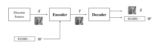
In RDH, bits of message are embedded by the encoder into the host sequence , by slightly modifying its elements to produce a stego sequence , where and , for , . This paper considers the convention that host signals and stego signals draw from the same set, i.e., . We denote the embedding capacity, also called embedding rate, by . Schemes are usually constructed to minimize some distortion measure between the host sequence and the stego sequence for a given embedding rate . The distortion metric in this paper is defined as the square error distortion, i.e., . The decoder can losslessly reconstruct the message and the host sequence from the stego sequence . Figure 1 shows the general framework of RDH on a gray-scale image , where is the stego image with some distortion after embedding .
II-B Related works
II-B1 A Near Optimal Coding Method using Arithmetic Coding
In our previous work [1], we proposed a backward and forward iterative (BFI) algorithm to estimate the optimal distribution of the stego signals. The BFI algorithm assumes that the host and stego signals draw from the same set, i.e., . Algorithm 1 gives the details. Notably, the BFI method controls an input parameter for various embedding rate and distortion pairs. The case admits the uniform distribution performing the maximal embedding rate, and another case generates an unchanged distribution with zero embedding rate.
Based on the result of the BFI algorithm, we proposed a coding scheme in [1] to embed a message into the host sequence by the given cumulative pmfs and . The coding framework is similar to arithmetic coding. The encoder maintains two values , to interpret the joint information of the host signal and the temporal information produced at the last step. At the initialization, the vector represents the information of the first host signal. At the -th step, the encoder transforms the vector and the next host to the stego signal and the next vector , expressed as . First, we need to find the possible within the interval , then if and only if . Second, for the case , the stego signal is determined. The determines the interval , which is larger than , so for lossless recovery, the decoder needs more information, expressed as the information vector for lossless decoding. One can see that in order to determine , the pmf needs to be known first, and it can be derived from the cumulative pmf , i.e., . The next host signal determines the interval , and we scale the information vector to to obtain , where
| (3) |
for , . Then, we proceed to process the next host signal.
For another case , the has several possible values corresponding to each interval of
The adaptive arithmetic decoding is applied on the binary representation of message to determine the value . To fit the usage requirement of arithmetic coding, the two ends of the vector are scaled to and , resulting in , where
The arithmetic decoder determines the value , and the corresponding residual information that depends on the is discussed below. For the case , the is within the interval , so we don’t have the residual information, and the updated vector is representing the next host signal. For the case , the residual information is interpreted as the vector , which is scaled into the interval to obtain the updated vector . For the case , the residual information is interpreted as the vector , which is scaled into the interval to obtain the updated vector . In summary, the updated vector is as follows:
and
We continue the above steps until there is no next host signal. When is designated, the encoder sends out a prefix-free code value with minimal code length, where
More details can be found in [1].
There are two observations from the above description. First, the practical implementation cannot store the real interval due to the machine precision. Therefore, our previous work maintained the variables and with length , where returns the greatest integer less than or equal to the input number, and . As the arithmetic coding proceeds, the gradually approaches the and the two values may coincide in certain cases. When and coincide, it is impossible to embed any data. That is, the usage of arithmetic coding here may suffer from computing precision problem. Second, it is necessary to transmit the cumulative pmfs and , or only transmit and use the BFI algorithm to generate . No matter which strategy is chosen, it costs an additional overhead proportional to the alphabet size.
II-B2 A Variant of ANS Coding (ANS-Variant) [26]
The key idea of the pure form ANS coding is to encode a sequence of input symbols into a single natural number (also called state), unlike arithmetic coding that operates on a fraction. Before encoding, ANS holds a start state . On a high level, the ANS encoder always maintains a state that can be modified by the encoding function : takes a symbol and the current state and produces a new state that encodes both the symbol and current state . Correspondingly, the decoding function decodes the state to a symbol and the previous state , i.e., . It is noted that the encoder and decoder in ANS coding go through the same sequence of states, just in opposite order. This paper uses the convention that the encoder processes symbols forward, from the first to the last, and the decoder recovers symbols backwards, from the last to the first.
Consider an input sequence , it is assumed that is a power of two, i.e. for an integer . This is a standard assumption like arithmetic coding for ANS coding to simplify arithmetic operations. In our recent work [26], we proposed a new ANS variant that forces the state always at a fixed interval by renormalization, where as long as . Let denote the interval corresponding to the symbol , which ensures that the new state after encoding symbol is within the interval . That is, if we have ; otherwise, we have . The encoding function is defined as . For the ease of understanding, the encoding procedure is assumed to be implemented using a stack, where each entry in the stack is a bit. Below gives the encoding details. To encode each symbol , if the current state is within , we first push -bit value to the stack and produce a new state by , where denotes the remainder operation. Otherwise, we first pop bits from the stack, and append them to the least significant bits of to increase it. That is, if the decimal representation of the popped bits is , we have . After that, we push -bit value to the stack and perform with the increased state . Notably, to ensure that there are enough bits in the stack before the first popping, we initialize the start state to be large enough, e.g., . We follow the above steps until all symbols are encoded. Finally, it is necessary to transmit the final state of encoding (which is also the start state of decoding) and the remaining bits in the stack to the decoder for lossless recovery.
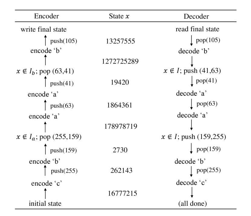
Next, we discuss the corresponding decoding details of our recent ANS-Variant coding. The decoding procedure can also be implemented using a stack, where each entry in the stack is also a bit. First, in order to completely reconstruct the input sequence , the decoder needs to know the statistics of the input sequence, including the total number of symbols, the frequency of each symbol and the selected fixed interval . Let if for and . Given a start state for decoding (i.e., the final state in the encoding) and the compressed bits stored in the stack, we pop -bit digit from the stack and decode it to a symbol , i.e., . Then, we update the state by , where . It can be seen that after a symbol is decoded, the value of state becomes larger. As more and more symbols get decoded, its value will eventually grow beyond a bound. When the state exceeds the upper bound chosen during the encoding, i.e., , we push the least significant bits of to the stack to make smaller, i.e., . We repeat the above steps, and the repetition stops when the reconstruction of input sequence is achieved. Figure 2 shows a worked-through example for a partial sequence “baabc" with parameters , and . The start state for encoding is chosen as . It can be seen that the encoder and decoder go through the same state just in opposite order. Also, the order of the symbols reconstructed by the decoder is opposite to that received by the encoder, e.g., the last encoded symbol is decoded first.
III Proposed Coding Scheme
The first limitation in our previous work [1] is that it uses arithmetic coding as the underlying coding framework. Arithmetic coding assigns each symbol to a sub-interval according to the probability of that symbol. When a symbol is encoded, the sub-interval narrows, and and move closer together. Because the machine system cannot represent infinite precision, as more and more symbols are encoded, gradually approaches and the two values eventually may coincide, then further data embedding is impossible. In this section, we first propose a coding method that employs our recent ANS variant [26] to embed a message into the host sequence . Then, the data extraction of the host sequence and the embedded message is given. Notably, this section considers the case where the statistics of the input sequence are known to the encoder and decoder, and refers to them as static data embedding and static data extraction. In the following, let and represent the values of host signal and stego signal at position in the sequence, respectively.
III-A Static Data Embedding
Our recent ANS-Variant coding (see Section II-B2 for details) can provide the compression ratio close to that of arithmetic coding. More importantly, it does not suffer from the computing precision problem that may occur in arithmetic coding. As a result, we adopt ANS-Variant as the coding framework to embed a message into the host sequence . The framework consists of a combination of an encoder and a decoder of ANS-Variant coding, where the encoder is used to embed the data, and the decoder returns the corresponding stego signals. From the description of ANS-Variant coding, one can see that in order to encode a host signal into the current state , the ANS-Variant encoder outputs an -bit value , and if the state is less than the lower bound of the selected fixed interval, the encoder reads bits to increase it. This observation can be exploited to realize data embedding, i.e., one can choose to read bits from the message to increase the value of the state if necessary. In addition, the BFI algorithm (described in Section II-B1) can estimate the optimal pmf of the stego sequence for a given host sequence. Therefore, we can apply the ANS-Variant decoder on the statistics of the stego sequence according to the -bit value to decode the corresponding stego signal . That is, the -bit value produced by the ANS-Variant encoder serves as the temporary information to decode the corresponding stego signal .
The details of the embedding procedure are as follows. First, we require knowledge of the host statistics and , and get the cumulative pmf , where and . Then, we apply the BFI algorithm on the to estimate the optimal cumulative pmf of the stego sequence . Once the distribution is known, we can further get the stego statistics and , where and . During the embedding, we process the host signals forward, i.e., from the first to the last signal. Given a start state , for each host signal , we first use an ANS-Variant encoder to encode it. Let and . During the encoding, we have the following two cases. In the first, if the current state , we read bits from the message to increase . That is, if the decimal representation of the bits read is , we have . After that, we maintain an -bit temporal information and update the state by . It is noted that the -bit temporary information produced by the host signal will be used in the following steps to decode the stego signal at the corresponding position. In the second, if the current state is within , we maintain an -bit temporal information and produce a new state by . Next, we utilize the temporary information maintained in the previous step and the stego statistics and to decode the corresponding stego signal . Precisely, we transmit the temporary information to an ANS-Variant decoder to decode the stego signal , i.e., . Then, we update the state by , where . From the description of ANS-Variant decoding in Section II-B2, one can see that the updated state has the following two cases. In the first, If the value of state exceeds the upper bound chosen during the encoding, we write the least significant bits of to the message to make smaller, i.e., . In the second, if the updated state is exactly within the interval , no further changes to the state are needed.
We repeat the above steps for the next host signal until there is no next host signal. As can be seen, an embedding cycle consists of a combination of an encoder and a decoder of ANS-Variant coding. Among them, the encoder aims to embed the data, and the decoder is designed to obtain the corresponding stego signal. Algorithm 2 presents the details. In Algorithm 2, Line aims to get the host statistics. Lines – first apply the BFI algorithm to estimate the optimal cumulative pmf and then get the stego statistics from the . In Line , the start state is chosen to be small enough, e.g., set to , in order to make the encoder read the bits from the message as early as possible, thus increasing the amount of embedded data. Lines – perform the encoding of ANS-Variant coding. In particular, Lines – read bits from the message to enlarge the state if the current state is too small. Lines – perform the decoding of ANS-Variant coding to generate the corresponding stego signal . Finally, we get a stego sequence and a final state . The final state needs to be transmitted along with the stego sequence , so that the extractor knows what state to start with. In addition, the shortened length (in bits) of the message is the amount of data embedded.
III-B Static Data Extraction
In RDH techniques, data extraction includes extracting the host sequence and the embedded message from the received stego sequence. In the proposed static data embedding (see Section III-A for details), we first perform ANS-Variant encoding based on the known host statistics, and then perform ANS-Variant decoding under the premise that the optimal cumulative pmf of the stego sequence has been estimated. The data extraction is just the inverse of data embedding. Therefore, in order to achieve lossless data extraction, we first perform the ANS-Variant encoding under the premise that the optimal cumulative pmf of the stego sequence is known. Then, we perform the ANS-Variant decoding based on the host statistics to decode the host signal. It is worth noting that the data extraction requires transmitting the cumulative pmfs and as parameters. Another strategy is to only transmit and the extractor generates the with the BFI algorithm. The latter saves space but requires a computational cost to run the BFI algorithm. This section takes the latter as an example to introduce the process of static data extraction.
Given a stego sequence , a start state , and the cumulative pmf , the details of data extraction are as follows. First, we apply the BFI algorithm on the host to estimate the optimal cumulative pmf . According to the and , we calculate the stego statistics and , and the host statistics and , where , , and , . These statistics are used in the subsequent encoding and decoding of ANS-Variant coding. As the encoder and decoder of ANS-Variant coding run in reverse order, we process the stego signals backwards, i.e., from the last to the first signal. For each stego signal , we first perform the ANS-Variant encoding based on the obtained stego statistics and . Specifically, let and . In the encoding, we have the following two cases. In the first, if the current state , we read bits from the message to increase . Then, we hold an -bit temporal information and update the state by . In the second, if the current state is within , we directly maintain an -bit temporal information and produce a new state by . The above -bit temporary information produced by encoding the stego signal is used in the following steps to decode the corresponding host signal .
Next, we utilize the temporary information maintained in the previous step and the host statistics and to decode the host signal . Precisely, we transmit the temporary information to the ANS-Variant decoder to decode the host signal , i.e., . Then, we update the state by , where . From the description of ANS-Variant decoding in Section II-B2, one can see that the updated state has the following two cases. In the first, if the value of state exceeds the upper bound chosen during the data embedding, we write the least significant bits of to the message to make smaller, i.e., . In the second, if the updated state is exactly within the interval , no further changes to the state are needed. We repeat the above steps for the next stego signal until there is no next stego signal. Algorithm 3 gives the details. In Algorithm 3, Line uses the BFI algorithm to estimate the optimal cumulative pmf . Lines – derive the host and stego statistics from the known and , respectively. Lines – perform the encoding of ANS-Variant coding on the stego signal and maintain a temporary information . Lines – utilize the temporary produced in the previous step to decode the host signal . In particular, Lines – write bits to the message when the state exceeds a given upper bound . Finally, we can reconstruct the host sequence and the embedded message without loss.
IV Dynamic Implementation
Section III presents the embedding/extraction procedure to embed a message in the i.i.d. host sequence. One can see that the proposed static RDH scheme, like our previous work [1], requires the cumulative pmf of the host sequence as a parameter in both the embedding/extraction process. Namely, the proposal involves using preset probabilities of signals that remain static during the whole process. However, transmitting the host pmf costs an additional overhead proportional to the alphabet size , which is usually unacceptable in extremely space-constrained scenarios. Moreover, the usability of the proposal is based on the premise that the pmf of the host sequence is known, imposing certain limitations on the practical application. In this section, we present a dynamic implementation without any prior knowledge of the host pmf. The implementation changes the probability after each host signal is encountered, thus saving the prior transmission of . First, we describe the dynamic data embedding algorithm. Second, the corresponding dynamic data extraction algorithm is given.
IV-A Dynamic Data Embedding
When any prior knowledge of the host pmf is not available, the proposed dynamic embedding method becomes a two-pass procedure. First, considering that the ANS-Variant decoder reconstructs all symbols in the reverse order of those processed by its encoder, so in order to ensure the synchronization of the encoder and the decoder, it is necessary to follow the order of the decoder run to collect the statistics of the host signal at each location. Therefore, we first pass the host sequence once in the decoder’s running order. Precisely, we start with a frequency distribution , e.g., , where denotes the number of occurrence of the signal . If the ANS-Variant decoder runs backwards, i.e., from the last to the first signal, we update the frequency distribution backwards based on the host signals encountered. Details of the update are as follows. We start with the last host signal and perform a backward pass over the host sequence. During the backward pass, when a host signal is encountered, the frequency corresponding to signal is updated via . Next, we backward continue with the next signal and update its frequency in the same manner. When the frequency of the first host signal is updated and there is no next host signal, we get the newest frequency distribution , which counts the frequency of each signal in the host sequence over the start frequency distribution.
When the first backward pass is completed, with the help of the newest statistics , we then use an ANS-Variant encoder followed by an ANS-Variant decoder to perform data embedding. The dynamic embedding procedure is similar to that of the static data embedding described in Section III-A, except that the dynamic version employs a changing pmf. Given a host sequence , a message to embed and the newest frequency distribution obtained in the first backward pass, the embedding details are described below. Considering that the encoder and decoder of the ANS-Variant coding run in opposite directions, and the first pass in the same order as the decoder runs is backwards, we perform a second forward pass (i.e., from the first to the last signal) on the host sequence. For each host signal encountered, we first update the corresponding frequency of signal by . Then, we compute the host statistics and the cumulative pmf from the newest . Next, we apply the BFI algorithm on the to estimate the optimal cumulative pmf of the stego sequence . Once the is known, we can also get the stego statistics and , where and . Once the host and stego statistics (i.e., , , and ) are both available, we then implement data embedding using similar steps in static data embedding (see Lines – in Algorithm 2 for details). We repeat the above steps for the next host signal until there is no next host signal. Finally, we get a stego sequence and a final frequency distribution . From the update rule of the , it can be seen that the final is exactly the same as the start before the first backward pass. Algorithm 4 gives the details. In Algorithm 4, Lines – initialize the frequency distribution to all ones and perform a backward pass. Line updates the frequency corresponding to the signal . Lines – first calculate the host statistics and , and then use the BFI algorithm to estimate the optimal . Line gets the stego statistics and from the . Lines – perform the encoding of ANS-Variant coding. In particular, Lines – read bits from the message to enlarge the state if it is too small. Lines – perform the decoding of ANS-Variant coding to obtain the corresponding stego signal . Finally, we get a stego sequence and a final state .
According to the above description, it is clear that the host pmf is not necessary in the proposed dynamic data embedding. Therefore, unlike our previous work [1], the proposed dynamic method overcomes the limitation of explicitly transmitting the host pmf , and brings flexibility in practical applications.
IV-B Dynamic Data Extraction
In order to reconstruct the host sequence and the embedded message from the stego sequence without any prior knowledge of the host pmf, the proposed dynamic data extraction also initializes a frequency distribution and changes it after a host signal is decoded. The start is exactly the same as the start before the first backward pass in the dynamic data embedding, i.e., we have , where denotes the number of occurrence of signal . The dynamic extraction procedure is similar to that of the static data extraction described in Section III-B, except that the dynamic version employs a changing pmf to save the prior transmission of the host pmf.
Given a stego sequence , a final state in the dynamic embedding, the details of the dynamic data extraction are as follows. First, we initialize the frequency distribution as . Then, considering that the encoder and decoder of the ANS-Variant coding run in the opposite directions, we process the stego signals backwards, i.e., from the last to the first signal. For each stego signal , we first get the statistics and the cumulative pmf from the newest , where and . Then, we adopt the BFI algorithm on the to estimate the optimal cumulative pmf . Once the is available, the corresponding stego statistics and can also be calculated, where and . Next, we implement data extraction using similar steps in static data extraction (see Lines – in Algorithm 3 for details). Notably, when a host signal is decoded, we need to update its frequency by . We repeat the above steps for the next stego signal until there is no next stego signal. Finally, we can reconstruct the host sequence and the embedded message. Algorithm 5 gives the details. In Algorithm 5, Line initializes to all ones. Line gets the host statistics and from the newest . Lines – first use the BFI algorithm to estimate the optimal and then get the stego statistics and from the . Lines – perform the ANS-Variant encoding on the stego signals and maintain a temporary information . Lines – utilize the temporary to decode the host signal and update the state . If the updated state exceeds the selected upper bound , Lines – write the least significant bits of to the message to decrease . Finally, Line updates the frequency of the corresponding host signal . From the above description, one can see that the dynamic data extraction procedure does not require any prior knowledge of the host pmf. It dynamically adjusts the pmf based on the decoded host signals to save the additional overhead.
V Simulations
In this section, we evaluate the embedding performance of the proposed static/dynamic method in terms of the mean squared error (MSE), embedding rate (in bits per pixel, bpp) and PSNR value (in dB) for images. The proposed methods are compared with three methods, including our previous work [1] and two high capacity RDH methods [20], [32]. The proposed methods are implemented in Visual C++ code with OpenCV image development kits. First, we show the experimental results on the i.i.d. sequence. Second, all experiments are conducted on gray-scale images (two common standard images of size 512 512).
V-A Experiments for i.i.d. Sequence
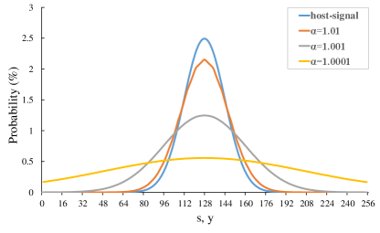
In this subsection, we test the embedding performance of the proposed static/dynamic method and our previous work [1] on i.i.d. sequence. We consider the host sequence drawn from discrete normal distribution. The host signals are -bit gray-scale with , and the mean of the normal distribution is at . Figure 3 shows the pmf of host signals for the standard deviation , and the pmf of stego signals by applying the BFI algorithm for and . It can be seen that the pmf of stego signals are more stationary than that of host signals, thus the stego sequence has a larger Shannon entropy. That is, more information is required on average to represent it, and the increased volume can be utilized to embed secret data.
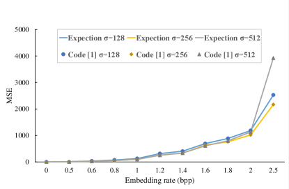
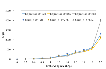
We adopt two common metrics embedding rate (bpp) and MSE to evaluate the embedding performance. For a host sequence and a stego sequence , the MSE is defined as
The lower the MSE value, the better the quality. The secret message is generated by multiple calls to the operation , which returns a pseudo-random number between (inclusive) and (exclusive). Figures 4–6 show the rate-distortion curves for the pmf with various . The blue line, yellow line and gray line, respectively, depict the expected rate-distortion curves for , and . We implement our previous work [1] (Code [1]), the proposed static method (Ours_s) and the proposed dynamic method (Ours_d) to embed the message in the host signals for each corresponding pmfs and , and the rate-distortion values are respectively marked as circles, rhombuses and triangles in Figures 4–6. In the proposed static/dynamic implementation, we use bits to represent the state and choose parameters , and . From Figures 4–5, one can see that the performance of the proposed static method is similar to that of our previous work [1], both approach the expected rate-distortion bound. More importantly, the proposed method uses ANS coding instead of arithmetic coding for RDH, which does not cause computing precision problems. Figure 6 gives the performance of the proposed dynamic method. It shows that the rate-distortion values in the dynamic version have a small distance from the expected rate-distortion bound. This is due to the fact that we use a predicted pmf instead of the true pmf. Especially, our proposal does not require transmitting the host pmf during data embedding and extraction, which saves additional overhead and enhances practicality.


V-B Experiments for Gray-Scale Images
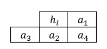
In this subsection, the embedding performance of the proposed static/dynamic method on gray-scale images is compared with three state-of-the-art methods, including our previous work [1] and two high capacity RDH methods [20] and [32]. To reduce the correlation of the neighboring image pixels, we preprocess the host image with predictive coding. The predictive coding processes the host pixels from left to right, and from top to bottom. Figure 7 shows a host image Lena and depicts the four neighboring pixels used for predicting the host pixel . The predicted value is defined as
| (4) |
For the pixels at the leftmost column, e.g, , we pick the nearby right pixel as the predicted value. For the pixels at the rightmost column, e.g, , we pick the nearby lower pixel as the predicted value. For the pixels at bottom row, e.g, , we pick the nearby right pixel as the predicted value. We omit the bottom-right corner pixel and default it to .
In order to embed a message into the host image, the existing RDH methods usually utilize the differences between the host and predicted pixels. However, these methods use Modulo operation to avoid the overflow/underflow problem, i.e., the values of some pixels in the stego image may exceed the upper or lower bound, e.g., or for an -bit gray-scale image. This may cause the stego image to suffer from the salt and pepper noise. To overcome this issue, we suggest to develop a two-dimensional lookup table K of size . The row index of the table denotes the predicted pixel and the column index denotes the true host pixel, where , . The entry at the -th row and the -th column in the table K represents the number of host pixel predicted as predicted pixel . Next, we give the details of static data embedding/extraction on gray-scale images. First, we initialize the two-dimensional table K to all ones, i.e., , where . Then, for each host pixel , we use the predictor to get its predicted value , and update the corresponding entry by . If the predictor works accurately enough, i.e., , one can see that the larger values in the table K will be clustered on the diagonal. When the two-dimensional table K has been built, we then embed the message into host image by utilizing the corresponding row as the host pmf. We process the host pixels from left to right, and from top to bottom. Specifically, for each host pixel , we first use the predictor to get its predicted value . Then, we take as the row index to look up the table K, and return a one-dimensional statistic of size . Afterwards, the is used as the frequency distribution to calculate the in Algorithm 2. Once the is available, we can embed the message by applying Algorithm 2. We repeat the above steps until there is no next host pixel. Finally, we can get a stego image. In the static data extraction, we reconstruct the host image in the reverse order from right to left, and from bottom to top. Consider the step of decoding shown in Figure 7b, the four neighboring host pixels , , and had been decoded by the previous decoding steps. Therefore, we have the predicted value through (4). Then, we take as the row index to look up the table K and return a one-dimensional statistic of size . Also, the is used as the frequency distribution to calculate the in Algorithm 3. Once the is available, we can perform the data extraction via Algorithm 3. We repeat the above steps until there is no next stego pixel. Finally, we can reconstruct the host image and embedded message.
Below, we discuss the details of dynamic data embedding/extraction on gray-scale images. First, we initialize a two-dimensional table K to all ones, i.e., , where . Then, we perform a backward pass over the host image, and for each host pixel , we use the predictor to obtain its predicted value . And, we update the corresponding entry in the table by . We repeat the above steps until there is no next host pixel. Next, the dynamic data embedding is implemented on the basis of the newest table K. We process the host pixels from left to right, and from top to bottom. Specifically, for each host pixel , we first use the predictor to get its predicted value . Notably, when a predicted value is obtained, we update the corresponding entry by . Then, we take as the row index to look up the table K and return a one-dimensional statistic of size . Afterwards, the is used as the frequency distribution to calculate the host statistics and in Line of Algorithm 4. Then, we can embed the message via Lines – in Algorithm 4. We repeat the above steps until there is no next host pixel, and finally we can get a stego image. In the corresponding dynamic data extraction, we first initialize a two-dimensional lookup table K to all ones, and predict the pixel in the reverse order from right to left, and from bottom to top. Similarly, we then take as the row index to look up the table K and return a statistic of size . The is used to calculate the host statistics and in Line of Algorithm 5. Then, we can decode the host pixel via Lines – in Algorithm 5. Notably, when a host pixel is decoded, we update the corresponding entry by . We repeat the above steps until all host pixels are decoded. Finally, the host image and the embedded message are reconstructed.
The PSNR (in dB) is often used as an objective measure of image quality, which reflects the degree of similarity between the stego image and host image. That is, the larger the value of PSNR, the better the image quality. The PSNR is calculated as
where is the maximum possible pixel value of the image (e.g., for -bit gray-scale images), and MSE is the mean squared error between the host and stego image. Given a noise-free host image and its stego image , MSE is defined as
where and represent the pixels at the -th row and the -th column in images and , respectively.


Next, we give the experimental results on gray-scale images. First, Figures 8–9 shows the embedding rate (bpp) and PSNR (dB) of the proposed static method on two sized standard gray-scale images, including Lena and Airplane from the USC_SIPI image database111https://sipi.usc.edu/database/, where the embedding rate is defined as the number of bits embedded divided by the number of pixels in the host image. The larger , the higher embedding capacity. It can be observed that when the embedded capacity decreases, the PSNR increases steadily.
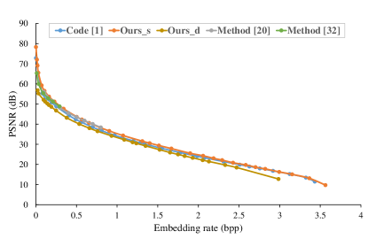
Second, we show the embedding performance of the proposed static/dynamic method, our previous work [1] and two high capacity RDH methods [20] and [32] on the test image Lena. We use bits to represent the state and choose parameters , and . The embedding performance with respect to the embedding rate versus the PSNR curve are plotted in Figure 10. It shows that for the same embedding capacity, the proposed static method provides slightly higher PSNR values than our previous work [1]. Compared with the method [20], our static method can achieve the similar performance at the low embedding rate. However, the method [20] states that it can only produce bpp on average, while the proposed method is capable to achieve larger embedding rates. Further, a location map is required in [20] to prevent the underflow/overflow problem, which brings additional storage consumption. Compared with the method [32], our static proposal can obtain a slight PSNR gain at the low embedding rate. But, the embedding capacity of the method [32] is relatively low, e.g., for the test image Lena, it has an embedding rate of at most bpp. In addition, the method [32] also requires a location map to avoid the underflow/overflow problem. For the proposed dynamic implementation, we initialize the two-dimensional lookup table K as follows: if ; otherwise, we have . As can be seen in Figure 10, the proposed dynamic method provides slightly lower PSNR values under the same embedding capacity. This observation is mainly due to the fact that we use the predicted pmf rather than the true pmf. More importantly, unlike our previous work [1], the proposed dynamic method does not require prior transmission of the host pmf during both embedding and extraction. In addition, compared with the existing methods [20], [32], our dynamic proposal also allows for larger embedding rates to achieve high capacity requirements.
VI Conclusion
In this paper, we proposed a novel RDH scheme based on our recent asymmetric numeral systems (ANS) variant [26]. To the best of our knowledge, this paper is the first that employs ANS coding for RDH technique. Unlike our previous work [1], the proposed method can completely avoid the computing precision problem. In addition, a dynamic implementation is also adaptively introduced to save the additional overhead of explicitly transmitting the host pmf during embedding and extraction. The experimental results show that the proposed static method provides slightly higher PSNR values than our previous work [1] and larger embedding rates than some state-of-the-art methods [20], [32] on gray-scale images. Besides, the proposed dynamic method saves additional overhead at the cost of a small image quality loss.
References
- [1] S.-J. Lin and W.-H. Chung, “The scalar scheme for reversible information-embedding in gray-scale signals: Capacity evaluation and code constructions,” IEEE Transactions on Information Forensics and Security, vol. 7, no. 4, pp. 1155–1167, 2012.
- [2] G. Gao, S. Tong, Z. Xia, B. Wu, L. Xu, and Z. Zhao, “Reversible data hiding with automatic contrast enhancement for medical images,” Signal Processing, vol. 178, pp. 1–14, 2021.
- [3] Z. Ni, Y. Q. Shi, N. Ansari, W. Su, Q. Sun, and X. Lin, “Robust lossless image data hiding designed for semi-fragile image authentication,” IEEE Transactions on Circuits and Systems for Video Technology, vol. 18, no. 4, pp. 497–509, 2008.
- [4] X. Li, B. Yang, and T. Zeng, “Efficient reversible watermarking based on adaptive prediction-error expansion and pixel selection,” IEEE Transactions on Image Processing, vol. 20, no. 12, pp. 3524–3533, 2011.
- [5] J. Tian, “Reversible data embedding using a difference expansion,” IEEE Transactions on Circuits and Systems for Video Technology, vol. 13, no. 8, pp. 890–896, 2003.
- [6] Y. Hu, H.-K. Lee, and J. Li, “De-based reversible data hiding with improved overflow location map,” IEEE Transactions on Circuits and Systems for Video Technology, vol. 19, no. 2, pp. 250–260, 2009.
- [7] W. He and Z. Cai, “Reversible data hiding based on dual pairwise prediction-error expansion,” IEEE Transactions on Image Processing, vol. 30, pp. 5045–5055, 2021.
- [8] S.-k. Lee, Y.-h. Suh, and Y.-s. Ho, “Reversible image authentication based on watermarking,” 2006 IEEE International Conference on Multimedia and Expo, pp. 1321–1324, 2006.
- [9] J. Wang, J. Ni, X. Zhang, and Y.-Q. Shi, “Rate and distortion optimization for reversible data hiding using multiple histogram shifting,” IEEE Transactions on Cybernetics, vol. 47, no. 2, pp. 315–326, 2017.
- [10] X. Li, B. Li, B. Yang, and T. Zeng, “General framework to histogram-shifting-based reversible data hiding,” IEEE Transactions on Image Processing, vol. 22, no. 6, pp. 2181–2191, 2013.
- [11] J. Wang, X. Chen, J. Ni, N. Mao, and Y. Shi, “Multiple histograms-based reversible data hiding: Framework and realization,” IEEE Transactions on Circuits and Systems for Video Technology, vol. 30, no. 8, pp. 2313–2328, 2020.
- [12] M. Celik, G. Sharma, A. Tekalp, and E. Saber, “Lossless generalized-lsb data embedding,” IEEE Transactions on Image Processing, vol. 14, no. 2, pp. 253–266, 2005.
- [13] W. Zhang, X. Hu, X. Li, and N. Yu, “Recursive histogram modification: Establishing equivalency between reversible data hiding and lossless data compression,” IEEE Transactions on Image Processing, vol. 22, no. 7, pp. 2775–2785, 2013.
- [14] C.-C. Lin, X.-L. Liu, W.-L. Tai, and S.-M. Yuan, “A novel reversible data hiding scheme based on ambtc compression technique,” Multimedia Tools and Applications, vol. 74, pp. 3823–3842, 2015.
- [15] W. Qi, S. Guo, and W. Hu, “Generic reversible visible watermarking via regularized graph fourier transform coding,” IEEE Transactions on Image Processing, vol. 31, pp. 691–705, 2022.
- [16] A. Alattar, “Reversible watermark using the difference expansion of a generalized integer transform,” IEEE Transactions on Image Processing, vol. 13, no. 8, pp. 1147–1156, 2004.
- [17] Z. Ni, Y.-Q. Shi, N. Ansari, and W. Su, “Reversible data hiding,” IEEE Transactions on Circuits and Systems for Video Technology, vol. 16, no. 3, pp. 354–362, 2006.
- [18] M. Fallahpour, “High capacity lossless data hiding based on histogram modification,” IEICE Electronics Express, vol. 4, no. 7, pp. 205–210, 2007.
- [19] W.-L. Tai, C.-M. Yeh, and C.-C. Chang, “Reversible data hiding based on histogram modification of pixel differences,” IEEE Transactions on Circuits and Systems for Video Technology, vol. 19, no. 6, pp. 906–910, 2009.
- [20] B. Ou and Y. Zhao, “High capacity reversible data hiding based on multiple histograms modification,” IEEE Transactions on Circuits and Systems for Video Technology, vol. 30, no. 8, pp. 2329–2342, 2020.
- [21] V. Manikandan, K. S. R. Murthy, B. Siddineni, N. Victor, P. K. R. Maddikunta, and S. Hakak, “A high-capacity reversible data-hiding scheme for medical image transmission using modified elias gamma encoding,” Electronics, vol. 11, no. 19, pp. 3101–3121, 2022.
- [22] T. Kalker and F. Willems, “Capacity bounds and constructions for reversible data-hiding,” 2002 14th International Conference on Digital Signal Processing Proceedings, vol. 1, pp. 71–76, 2002.
- [23] F. Willems, D. Maas, and T. Kalker, “Semantic lossless source coding,” 42nd Annual Allerton Conference on Communication, Control and Computing, 2004.
- [24] J. J. Rissanen, “Generalized kraft inequality and arithmetic coding,” IBM Journal of Research and Development, vol. 20, no. 3, pp. 198–203, 1976.
- [25] X. Hu, W. Zhang, X. Hu, N. Yu, X. Zhao, and F. Li, “Fast estimation of optimal marked-signal distribution for reversible data hiding,” IEEE Transactions on Information Forensics and Security, vol. 8, no. 5, pp. 779–788, 2013.
- [26] N. Wang, W. Yan, S.-J. Lin, and Y. Huang, “An entropy coding based on binary encoding for mixed-radix digits,” 2022 Data Compression Conference (DCC), pp. 488–488, 2022.
- [27] J. Duda, “Asymmetric numeral systems,” arXiv preprint arXiv:0902.0271, 2009.
- [28] J. Duda, K. Tahboub, N. J. Gadgil, and E. J. Delp, “The use of asymmetric numeral systems as an accurate replacement for huffman coding,” 2015 Picture Coding Symposium (PCS), pp. 65–69, 2015.
- [29] S. Camtepe, J. Duda, A. Mahboubi, P. Morawiecki, S. Nepal, M. Pawłowski, and J. Pieprzyk, “Compcrypt–lightweight ans-based compression and encryption,” IEEE Transactions on Information Forensics and Security, vol. 16, pp. 3859–3873, 2021.
- [30] D. Dubé and H. Yokoo, “Fast construction of almost optimal symbol distributions for asymmetric numeral systems,” 2019 IEEE International Symposium on Information Theory (ISIT), pp. 1682–1686, 2019.
- [31] D. A. Huffman, “A method for the construction of minimum-redundancy codes,” Proceedings of the IRE, vol. 40, no. 9, pp. 1098–1101, 1952.
- [32] Y. Jia, Z. Yin, X. Zhang, and Y. Luo, “Reversible data hiding based on reducing invalid shifting of pixels in histogram shifting,” Signal Processing, vol. 163, pp. 238–246, 2019.