\csdef

WGMwgm \csdefQEqe \csdefEPep \csdefPMSpms \csdefBECbec \csdefDEde \shorttitleA number-theoretic method sampling NN \shortauthorsYu Yang et al.

\tnotemark

[1]

¹¹footnotetext: This research is partially sponsored by the National key R & D Program of China (No.2022YFE03040002) and the National Natural Science Foundation of China (No.11971020, No.12371434).

[type=editor, auid=000,bioid=1, orcid=0009-0005-1428-6745 ]

[style=chinese]

\cormark

[1]

[style=chinese]

\cormark

[1]

A number-theoretic method sampling neural network for solving partial differential equations

Yu Yang yangyu1@stu.scu.edu.cn School of Mathematics, Sichuan University, 610065, Chengdu, China. Pingan He t330202702@mail.uic.edu.cn Faculty of Science and Technology, BNU-HKBU United International College, 519087, Zhuhai, China. Xiaoling Peng xlpeng@uic.edu.cn Guangdong Provincial Key Laboratory of Interdisciplinary Research and Application for Data Science, BNU-HKBU United International College, 519087, Zhuhai, China Qiaolin He qlhejenny@scu.edu.cn

Abstract

When dealing with a large number of points, the widely used uniform random sampling approach for approximating integrals using the Monte Carlo method becomes inefficient. In this work, we develop a deep learning framework established in a set of points generated from the number-theoretic method, which is a deterministic and robust sampling approach. This framework is designed to address low-regularity and high-dimensional partial differential equations, where Physics-Informed neural networks are incorporated. Furthermore, rigorous mathematical proofs are provided to validate the error bound of our method is less than that of uniform random sampling method. We employ numerical experiments involving the Poisson equation with low regularity, the two-dimensional inverse Helmholtz equation, and high-dimensional linear and nonlinear problems to illustrate the effectiveness of our algorithm.

{keywords}

deep learning , neural network , partial differential equation , sampling , good lattice points

1 Introduction

Numerically solving partial differential equations (PDEs) [29] has always been one of the concerns of frontier research. In recent years, as the computational efficiency of hardware continues to improve, the approach of utilizing deep learning to solve PDEs has increasingly gained attention. The neural networks with enhanced knowledge and the deep Galerkin method were introduced in references [28] and [31], respectively. The Deep Ritz method, which is grounded in the variational formulation of PDEs, was developed in [36]. The deep backward stochastic differential equations (BSDEs) framework, adept at addressing high-dimensional PDEs, was established in [10] based on stochastic differential equations(SDEs). From the perspective of operator learning, deep operator networks (DeepONet) were proposed in [21], and the Fourier Neural Operator (FNO) framework was introduced in [19]. In this work, we are concerned with Physics-Informed Neural Networks (PINNs)[28].

For the general PINN, its network structure is a common fully connected neural network, the input is the sampling points in the computational domain, and the output is the predicted solution of PDEs. Its loss function is usually made up of the norm $L_{2}$ of the residual function of PDEs, the boundary loss and more relevant physical constraints. The neural network is then trained by an optimization method to approximate the solution of PDEs. At present, it is a widely accepted fact that the error of PINNs is composed of three components [30] which are approximation error, estimation error and optimization error, where the estimation error is due to the Monte Carlo (MC) method to discretize the loss function.

Our goal is to improve the prediction performance of PINNs by reducing the estimation error. When using MC method to discretize the loss function in integral form, sampling points obeying a uniform distribution are usually sampled to serve as empirical loss, which may cause large error. It is then worth considering how to get better sampling. Currently, there have been many works on non-uniform adaptive sampling. In the work [22], the residual-based adaptive refinement (RAR) method aimed at enhancing the training efficiency of PINNs is introduced. Specifically, this method adaptively adds training points in regions where the residual loss is large. In [37], a novel residual-based adaptive distribution (RAD) method is proposed. The main concept of this method involves constructing a probability density function that relies on residual information and subsequently employing adaptive sampling techniques in accordance with this density function. An adaptive sampling framework for solving PDEs is proposed in [35], which formulating a variance of the residual loss and leveraging KRNet, as introduced in [34]s. Contrary to the methods mentioned above that rely on residual loss, an MMPDE-Net grounded in the moving mesh method in [38] is proposed, which cleverly utilizes the information from the solution to create a monitor function, facilitating adaptive sampling of training points.

Compared to non-uniform adaptive sampling, uniform non-adaptive sampling does not require a pre-training step to obtain information about the loss function or the solution, which directly improves efficiency. There are several common methods of uniform non-adaptive sampling, which include 1) equispaced uniform points sampling, a method that uniformly selects points from an array of evenly spaced points, frequently employed in addressing low-dimensional problems; 2) Latin hypercube sampling (LHS, [33]), which is a stratified sampling method based on multivariate parameter distributions; 3) uniform random sampling, which draws points at random in accordance with a continuous uniform distribution within the computational domain, representing the most widely adopted method ([14, 18, 28]).

In this work, we develop a uniform non-adaptive sampling framework, according to number-theoretic methods (NTM), which is introduced by Korobov [16]. It is a method based on number theory to produce uniformly distributed points, which is used to reduce the need for sampling points when calculating numerical integrals. Later on, researchers found that the NTM and the MC method share some commonalities in terms of uniform sampling, so it is also known as the quasi-Monte Carlo (QMC) method. In NTM, there are several types of low-discrepancy point sets, such as Halton sequences [8], Hammersley sequences [9], Sobol sequences [32] and good lattice point set [16]. Among them, we are mainly concerned with the good lattice point set (GLP set). The GLP set is introduced by Korobov for the numerical simulations of multiple integrals [16], and it has been widely applied in NTM. Subsequently, Fang et al. introduced the GLP set into uniform design ([6, 5]), leading to a significant development. Compared to uniform random sampling, the GLP set offers the following advantages: (1) The GLP set is established on the NTM, and once the generating vectors are determined, its points are deterministic. (2) The GLP set has higher uniformity, which is attributed to its low-discrepancy property. This advantage becomes more pronounced in high-dimensional cases, as the GLP set can be uniformly cattered throughout the space, which is difficult to do with uniform random sampling. (3) The error bound of the GLP set is better than that of uniform random sampling in numerical integrations. It is well known ([2, 4, 27]) that the MC method approximates the integral with an error of $\bm{O}\left(N^{-\frac{1}{2}}\right)$ when discretizing the integral using $N$ i.i.d random points. With $N$ deterministic points, the GLP set approximates the integral with an error of $\bm{O}\left(\frac{(\log N)^{d}}{N}\right)$ , where $d$ is the dimension of the integral (see Lemma 2). Thus, for the same number of sampling points, the GLP set performs better than uniform random sampling. When using PINNs to solve the PDEs, a large number of sampling points may be required, such as low regularity problems or high dimensional problems. In such case, the uniform random sampling is very inefficient. In this work, GLP sampling is utilized instead of uniform random sampling, which not only reduces the consumption of computational resources, but also improves the accuracy. Meanwhile, we also give an upper bound about the error of the predicted solution of PINNs when using GLP sampling through rigorous mathematical proofs. According to the error upper bound, we prove that GLP sampling is more effective than uniform random sampling.

The rest of the paper is organized as follows. In Section 2, we will give the problem formulation of PDEs and a brief review of PINNs. In Section 3, we will describe GLP sampling and also present the neural network framework incorporating GLP sampling and give the error estimation. Numerical experiments are shown in Section 4 to verify the effectiveness of our method. Finally, conclusions are given in Section 5.

2 Preliminary Work

2.1 Problem formulation

The general formulation of the PDE problem is as follows

\left\{\begin{aligned} \mathcal{A}[\bm{u}(\bm{x})]&=f(\bm{x}),\quad\bm{x}\in\Omega,\\ \mathcal{B}[\bm{u}(\bm{x})]&=g(\bm{x}),\quad\bm{x}\in\partial\Omega.\end{aligned}\right.

(1)

where $\Omega\subset\mathbb{R}^{d}$ represents a bounded, open and connected domain which surrounded by a polygonal boundary $\partial\Omega$ . And $\bm{u}(\bm{x})$ is the unique solution of this problem. There are two partial differential operators $\mathcal{A}$ and $\mathcal{B}$ defined in $\Omega$ and on $\partial\Omega$ , the $f(\bm{x})$ is the source function within $\Omega$ and $g(\bm{x})$ represents the boundary conditions on $\partial\Omega$ .

2.2 Introduction to PINNs

For a general PINN, its input consists of sampling points $\bm{x}$ located within the domain $\Omega$ and on its boundary $\partial\Omega$ , and its output is the predicted solution $\bm{u}(\bm{x};\theta)$ , where $\theta$ represents the parameters of the neural network, typically comprising weights and biases. Suppose that $\mathcal{A}[\bm{u}(\bm{x};\theta)]-f(\bm{x})\in\mathbb{L_{2}}(\Omega)$ and $\mathcal{B}[\bm{u}(\bm{x};\theta)]-g(\bm{x})\in\mathbb{L_{2}}(\partial\Omega)$ , the loss function can be expressed as

$\displaystyle\mathcal{L}(\bm{x};\theta)$	$\displaystyle=\alpha_{1}\\|\mathcal{A}[\bm{u}(\bm{x};\theta)]-f(\bm{x})\\|_{2,\Omega}^{2}+\alpha_{2}\\|\mathcal{B}[\bm{u}(\bm{x};\theta)]-g(\bm{x})\\|_{2,\partial\Omega}^{2}$	(2)
	$\displaystyle=\alpha_{1}\int_{\Omega}\|\mathcal{A}[\bm{u}(\bm{x};\theta)]-f(\bm{x})\|^{2}d\bm{x}+\alpha_{2}\int_{\partial\Omega}\|\mathcal{B}[\bm{u}(\bm{x};\theta)]-g(\bm{x})\|^{2}d\bm{x}$
	$\displaystyle\triangleq\alpha_{1}\int_{\Omega}\|r(\bm{x};\theta)\|^{2}d\bm{x}+\alpha_{2}\int_{\partial\Omega}\|b(\bm{x};\theta)\|^{2}d\bm{x}$
	$\displaystyle\triangleq\alpha_{1}\mathcal{L}_{r}(\bm{x};\theta)+\alpha_{2}\mathcal{L}_{b}(\bm{x};\theta),$

where $\alpha_{1}$ is the weight of the residual loss $\mathcal{L}_{r}(\bm{x};\theta)$ and $\alpha_{2}$ is the weight of the boundary loss $\mathcal{L}_{b}(\bm{x};\theta)$ .

We use the residual loss $\mathcal{L}_{r}(\bm{x};\theta)$ as an example of how to discretize by Monte Carlo method.

$\displaystyle\mathcal{L}_{r}(\bm{x};\theta)$	$\displaystyle=\int_{\Omega}\|r(\bm{x};\theta)\|^{2}d\bm{x}=V(\Omega)\int_{\Omega}\|r(\bm{x};\theta)\|^{2}U(\Omega)d\bm{x}$	(3)
	$\displaystyle=V(\Omega)\mathbb{E}_{\bm{x}\sim U}(\|r(\bm{x};\theta)\|^{2})$
	$\displaystyle\approx V(\Omega)\frac{1}{N_{r}}\sum_{i=1}^{N_{r}}\|r(x_{i};\theta)\|^{2},\quad\bm{x}\sim U(\Omega),$

where $V$ is the volume, $U$ is the uniform distribution, and $\mathbb{E}$ is the mathematical expectation. Thus, after sampling uniformly distributed residual training points $\left\{\bm{x}_{i}\right\}_{i=1}^{N_{r}}\subset\Omega$ and boundary training points $\left\{\bm{x}_{i}\right\}_{i=1}^{N_{b}}\subset\partial\Omega$ , the following empirical loss can be written as

\mathcal{L}_{N}(\bm{x};\theta)=\frac{\alpha_{1}V(\Omega)}{N_{r}}\sum_{i=1}^{N_{r}}|r(\bm{x}_{i};\theta)|^{2}+\frac{\alpha_{2}V(\Omega)}{N_{b}}\sum_{i=1}^{N_{b}}|b(\bm{x}_{i};\theta)|^{2},\quad N=N_{r}+N_{b}.

(4)

Finally, we usually use gradient descent methods, such as Adam [15] and LBFGS [20], to optimize for empirical loss $\mathcal{L}_{N}(\bm{x};\theta)$ .

3 Main Work

3.1 Method

In NTM, a criterion is necessary to measure how the sampling points are scattered in space, which is called discrepancy. There are many types of discrepancy, such as discrepancy based on uniform distribution, F-discrepancy that can measure non-uniform distributions, and star discrepancy that considers all rectangles, among others [5]. The discrepancy $D(N,X_{N})$ described in Definition 1 is used to describe the uniformity of a point set $X_{N}$ on the unit cube $C^{d}=[0,1]^{d}$ . For a point set $X_{N}$ , the smaller its discrepancy, the higher the uniformity of this point set, and the better it represents the uniform distribution $U(C^{d})$ . Therefore, the definition of good lattice point set generated from number-theoretic method is introduced.

Definition 1.

[6] Let $X_{N}=\left\{x_{i}\right\}_{i=1}^{N}$ be a set of points on $C^{d}$ . For a vector $\gamma\in C^{d}$ , let $K(\gamma,X_{N})$ denotes the number of points in $X_{N}$ that satisfy $x_{i}<\gamma$ . Then there is

D(N,X_{N})=\sup_{\gamma\in C^{d}}\left|\frac{K(\gamma,X_{N})}{N}-V\left([0,\gamma]\right)\right|,

(5)

which is called the discrepancy of $X_{N}$ , where $V\left([0,\gamma]\right)$ denotes the volume of the rectangle formed by the vector $\gamma$ from 0.

Definition 2.

[6] Let $GV=(N;h_{1},h_{2},...,h_{s})\in C^{d}$ to be a vector of integers that satisfy $1\leq h_{i}<N$ , $h_{i}\neq h_{j}(i\neq j)$ , $d<N$ and the greatest common divisor $(N,h_{i})=1,i=1,...,d$ . Let

\left\{\begin{aligned} q_{ij}&\equiv ih_{j}\pmod{N},\\ x_{ij}&=\frac{2q_{ij}-1}{2N},\quad i=1,...,N,\ j=1,...,d,\end{aligned}\right.

(6)

where $q_{ij}$ satisfies $1\leq q_{ij}\leq N$ . Then the point set $X_{N}=\left\{x_{i}=(x_{i1},x_{i2},...,x_{id}),i=1,...,N\right\}$ is called the lattice point set of the generating vector $GV$ . And a lattice point set $X_{N}$ is a good lattice point set if $X_{N}$ has the smallest discrepancy $D(N,X_{N})$ among all possible generating vectors.

Definition 2 shows that GLP set have an excellent low discrepancy. Usually, the lattice points of an arbitrary generating vector are not uniformly scattered. Then, an important problem is how to choose the appropriate generating vectors to generate the GLP set via Eq (6). According to ([17, 12]), there is a fact that for a given prime number $P$ , there is a vector $(h_{1},h_{2},...,h_{s})$ can be chosen such that the lattice point set of $(P;h_{1},h_{2},...,h_{s})$ is GLP set.

Lemma 1.

[13] For any given prime number $P$ , there is an integral vector $(h_{1},h_{2},...,h_{s})$ such that the lattice point set $X_{P}$ of $(P;h_{1},h_{2},...,h_{s})$ has discrepancy

D(P,X_{P})\leq pc(d)\frac{(\log P)^{d}}{P},

where $pc(d)$ denotes a positive constant depending on the dimension of the unit cube $C^{d}$ .

The proof of Lemma 1 can be found in [13]. Now, we consider how to find the generating vector on the basis of the Lemma 1. One feasible method ([17, 26]) is described as follows. For a lattice point set $X_{N}$ whose cardinality is a certain prime number $N=P$ , the generating vector can be constructed in the form $GV=(P;1,h_{1},h_{2},...,h_{s})$ , where $(h_{1},h_{2},...,h_{s})\equiv(1,a,a^{2},...,a^{d-1})\pmod{P}$ , $1<a<P$ . By finding a certain special primitive root $a$ among the primitive roots modulo $P$ , so that the lattice point set corresponding to $GV$ has the smallest discrepancy. If the number of sampling points is only prime, this may not satisfy our needs in many cases, and the more general case is considered below. When $N=2,4,P^{l},2P^{l}$ , where $P>2$ is a prime and $1\leq l$ , it is known that there must exist primitive roots mod $N$ . Moreover, the number of primitive roots is $\phi(\phi(N))$ , where $\phi(N)$ denotes the cardinality of the set $\{i|1\leq i<N,(i,N)=1\}$ . Since the GLP set is very efficient and convenient, a number of generate vectors corresponding to some good lattice point sets on unit cubes in different dimensions have already been presented in [13].

After getting the GLP set, we now discuss the calculation of the loss function of PINNs. Since the boundary loss usually accounts for a relatively small percentage of the total and can even be completely equal to 0 by forcing the boundary conditions([23], [24]), we focus on residual loss in the following. According to the central limit theorem and the Koksma-Hlawka inequality [11], we have the following lemma (more details can be found in [27]).

Lemma 2.

(i) If $f(\bm{x})\in\mathbb{L_{2}}(C^{d})$ and $\left\{\bm{x}_{i}\right\}_{i=1}^{N}\subset C^{d}$ is a set of i.i.d. uniformly distributed random points, then there is

\int_{C^{d}}f^{2}(\bm{x})d\bm{x}\leq\frac{1}{N}\sum_{i=1}^{N}f^{2}(x_{i})+\bm{O}\left(N^{-\frac{1}{2}}\right).

(ii) If $f(\bm{x})$ over $C^{d}$ has bounded variation in the sense of Hardy and Krause and $\left\{\bm{x}_{i}\right\}_{i=1}^{N}\subset[0,1)^{d}$ is a good lattice point set, then there is

\int_{C^{d}}f^{2}(\bm{x})d\bm{x}\leq\frac{1}{N}\sum_{i=1}^{N}f^{2}(x_{i})+\bm{O}\left(\frac{(\log N)^{d}}{N}\right).

Remark 1.

(1) In Lemma 2(i), the error bound is a probabilistic error bound of the form $\bm{O}\left(N^{-\frac{1}{2}}\right)$ in terms of $N$ . (2) According to [11] and [7], a sufficient condition for a function f to have bounded variance in the Hardy-Krause sense is that f has continuous mixed partial differential derivatives. In fact, some common activation functions in neural networks, such as the hyperbolic tangent function and the Sigmoid function, they are infinite order derivable. Therefore, when the activation functions mentioned above are chosen, the function $r(\bm{x};\theta)$ and $b(\bm{x};\theta)$ induced by the predicted solutions $\bm{u}(\bm{x};\theta)$ generated by the PINNs also satisfies the conditions of Lemma 2(ii) (similar comments can be found in [25].).

Recalling Eq (3), the discrete residual loss in $\Omega=(0,1)^{d}$ using uniform sampling can be written as

\displaystyle\mathcal{L}_{r}(\bm{x};\theta)

\displaystyle=\int_{\Omega}|r(\bm{x};\theta)|^{2}d\bm{x}=\mathbb{E}_{\bm{x}\sim U}(|r(\bm{x};\theta)|^{2})\approx\frac{1}{N_{r}}\sum_{i=1}^{N_{r}}|r(x_{i};\theta)|^{2},\quad\bm{x}\sim U(\Omega).

(7)

Given a good lattice point set $X_{N_{r}}=\left\{\bm{x}_{i}\right\}_{i=1}^{N_{r}}\subset\Omega$ , there is a discrete residual loss defined in Eq (8). In notation, we use superscripts to distinguish between sampling methods, where GLP denotes good lattice point set sampling and UR denotes uniform random sampling.

\mathcal{L}_{r,N_{r}}^{GLP}(\bm{x};\theta)=\frac{1}{N_{r}}\sum_{i=1}^{N_{r}}|r(x_{i};\theta)|^{2},x_{i}\in X_{N_{r}}.

(8)

If the conditions of Lemma 2 are satisfied, the error bound between $\mathcal{L}_{r,N_{r}}$ and $\mathcal{L}_{r}$ using GLP sampling will be smaller than the error using uniform random sampling when there are enough training points, which will result in smaller error estimate presented in Section 3.2. According to Eq (4), we have the following loss function.

\mathcal{L}_{N}(\bm{x};\theta)=\alpha_{1}\mathcal{L}_{r,N_{r}}^{GLP}(\bm{x};\theta)+\alpha_{2}\mathcal{L}_{b,N_{b}}^{UR}(\bm{x};\theta),\quad N=N_{r}+N_{b}.

(9)

Finally, the gradient descent method is used to optimize the loss function Eq (9). The flow of our approach is summarized in Algorithm 1 and Fig 1.

Symbols: Maximum epoch number of PINNs training:

M

; the numbers of total points in

\Omega

and

\partial\Omega

N_{r}

and

N_{b}

; generating vector:

GV=(N_{r};h_{1},h_{2},....,h_{d})

; uniform boundary training points

\mathcal{X}_{N_{b}}:=\left\{\bm{x}_{k}\right\}_{k=1}^{N_{b}}\subset\partial\Omega

; the number of test set points:

N_{T}

; test set

\mathcal{X}_{T}:=\left\{\bm{x}_{k}\right\}_{k=1}^{N_{T}}\subset\Omega\cup\partial\Omega

; the parameters of PINNs:

\theta

Sampling:

Input generating vector

GV=(N_{r};h_{1},h_{2},....,h_{d})

for the GLP set.

x_{ij}=\frac{2q_{ij}-1}{2N_{r}}

, where

q_{ij}\equiv ih_{j}\pmod{N_{r}},\quad i=1,...,N_{r},j=1,...,d.

Get the GLP set as the training set

\mathcal{X}_{N_{r}}:=\left\{x_{k}=(x_{k1},x_{k2},...,x_{kd})\right\}_{k=1}^{N_{r}}\subset\Omega

Training:

Input

\mathcal{X}_{N}:=\mathcal{X}_{N_{r}}\cup\mathcal{X}_{N_{b}}

into PINNs.

Initialize the output

\bm{u}\left(\mathcal{X}_{N};\theta_{1}\right)

for $i=1:M$ do

\mathcal{L}_{N}\left(\mathcal{X}_{N};\theta_{i}\right)=\alpha_{1}\mathcal{L}_{r,N_{r}}^{GLP}\left(\mathcal{X}_{N_{r}};\theta_{i}\right)+\alpha_{2}\mathcal{L}_{b,N_{b}}^{UR}\left(\mathcal{X}_{N_{b}};\theta_{i}\right)

;

Update

\theta_{i+1}

by optimizing

\mathcal{L}_{N}\left(\mathcal{X}_{N};\theta_{i}\right)

end for

Testing:

Input test set

\mathcal{X}_{T}

into PINNs.

Output

u(\mathcal{X}_{T};\theta_{M+1})

Algorithm 1 Algorithm of PINNs on GLP set

Refer to caption — Figure 1: Flow chart of our method.

3.2 Error Estimation

We consider the problem Eq (1) and assume that both $\mathcal{A}$ and $\mathcal{B}$ are linear operators. In this work, no matter how the set of points is formed, the uniform distribution sampling approach is utilized. And without loss of generality, in all subsequent derivations, we choose $\Omega=(0,1)^{d}$ , and $\alpha_{1}=\alpha_{2}=1$ in Algorithm 1.

Assumption 1.

(Lipschitz continuity) For any bounded neural network parameters $\theta_{1}$ and $\theta_{2}$ , there exists a postive constant $\mathbf{L}$ such that the empirical loss function satisfies

\|\nabla\mathcal{L}_{N}(\bm{x};\theta_{1})-\nabla\mathcal{L}_{N}(\bm{x};\theta_{2})\|_{2}\leq\mathbf{L}\|\theta_{1}-\theta_{2}\|_{2}.

(10)

Assumption 1 is a common assumption in optimization analysis since it is critical to derive Eq (11), which is known as descent lemma.

\mathcal{L}_{N}(\bm{x};\theta_{1})\leq\mathcal{L}_{N}(\bm{x};\theta_{2})+\nabla\mathcal{L}_{N}(\bm{x};\theta_{2})^{T}(\theta_{1}-\theta_{2})+\frac{1}{2}\mathbf{L}\|\theta_{1}-\theta_{2}\|_{2}^{2}.

(11)

Assumption 2.

For any bounded neural network parameters $\theta_{1}$ and $\theta_{2}$ , there exists a constant c such that the empirical loss function satisfies

\mathcal{L}_{N}(\bm{x};\theta_{1})\geq\mathcal{L}_{N}(\bm{x};\theta_{2})+\nabla\mathcal{L}_{N}(\bm{x};\theta_{2})^{T}(\theta_{1}-\theta_{2})+\frac{c}{2}\|\theta_{1}-\theta_{2}\|_{2}^{2}.

(12)

Assumption 2 states that the empirical loss function is strongly convex with respect to $\theta$ and Eq (12) is assumed similar as in references [1, 3]. Actually, the empirical loss function of neural networks is not always strongly convex, such as when using deep hidden layers and some nonlinear activation functions. However, the strong convexity shown in Assumption 2 is necessary to obtain Eq (13).

2c(\mathcal{L}_{N}(\bm{x};\theta)-\mathcal{L}_{N}(\bm{x};\theta^{*}))\leq\|\mathcal{L}_{N}(\bm{x};\theta)\|_{2}^{2},\ c\leq\mathbf{L},

(13)

where $\theta^{*}$ is the unique global minimizer. If the stochastic gradient descent method is utilized, the parameter update equation at the i+1st iteration in the general stochastic gradient descent method is given by

\theta_{i+1}=\theta_{i}-\eta_{i}g(x_{i},\theta_{i}),

where $\eta_{i}$ is the step size at the i+1st iteration. Same as the reference [3], we give the following assumption about the stochastic gradient vector $g(x_{i},\theta_{i}):=\frac{\partial\mathcal{L}_{N}((x_{i};\theta_{i}))}{\partial\theta_{i}}$ .

Assumption 3.

For the stochastic gradient vector $g(x_{i},\theta_{i}):=\frac{\partial\mathcal{L}_{N}((x_{i};\theta_{i}))}{\partial\theta_{i}}$ , $\forall i\in\mathbb{N}^{+}$ ,

(i) there exists $0<\mu\leq\mu_{G}$ such that the expectation $\mathbb{E}_{x_{i}}\left(g(x_{i},\theta_{i})\right)$ satisfies

	$\displaystyle\nabla\mathcal{L}_{N}(\bm{x};\theta_{i})^{T}\mathbb{E}_{x_{i}}\left(g(x_{i},\theta_{i})\right)\geq\mu(1+s(N_{r},N_{b}))\\|\nabla\mathcal{L}_{N}(\bm{x};\theta_{i})\\|_{2}^{2},$		(14)
	$\displaystyle\\|\mathbb{E}_{x_{i}}\left(g(x_{i},\theta_{i})\right)\\|_{2}\leq\mu_{G}(1+s(N_{r},N_{b}))\\|\nabla\mathcal{L}_{N}(\bm{x};\theta_{i})\\|_{2}.$		(15)

(ii) there exist $C_{V}\geq 0$ and $M_{V}\geq 0$ such that the variance $\mathbb{V}_{x_{i}}\left(g(x_{i},\theta_{i})\right)$ satisfies

\mathbb{V}_{x_{i}}\left(g(x_{i},\theta_{i})\right)\leq C_{V}R(N_{r},N_{b})+M_{V}(1+s(N_{r},N_{b}))\|\nabla\mathcal{L}_{N}(\bm{x};\theta_{i})\|_{2}^{2}.

(16)

In Assumption 3, the $s(N_{r},N_{b})$ is the square of the error between the empirical loss function $\mathcal{L}_{N}$ and the loss function in integral form $\mathcal{L}$ . For example, if the conditions of Lemma 2 are satisfied, the $s(N_{r},N_{b})=\left(\bm{O}\left({N_{r}}^{-\frac{1}{2}}\right)+\bm{O}\left({N_{d}}^{-\frac{1}{2}}\right)\right)^{2}$ for the uniform random sampling and $s(N_{r},N_{b})=\left(\bm{O}\left(\frac{(\log N_{r})^{d}}{N_{r}}\right)+\bm{O}\left({N_{d}}^{-\frac{1}{2}}\right)\right)^{2}$ for the GLP set.

Theorem 1.

Suppose that the stepsize $\eta$ is fixed and it satisfies

0<\eta\leq\frac{\mu}{\mathbf{L}\left(M_{V}+\mu^{2}_{G}(1+s(N_{r},N_{b}))\right)},

(17)

and under assumptions (1,2 and 3), there is

\lim_{i\to\infty}\mathbb{E}\left(\mathcal{L}_{N}(\bm{x};\theta_{i})\right)=\frac{\eta\mathbf{L}C_{V}}{2c\mu}s(N_{r},N_{b}).

(18)

Proof.

Using Eq (11), we have

\mathcal{L}_{N}(\bm{x};\theta_{i+1})\leq\mathcal{L}_{N}(\bm{x};\theta_{i})+\nabla\mathcal{L}_{N}(\bm{x};\theta_{i})^{T}(\theta_{i+1}-\theta_{i})+\frac{1}{2}\mathbf{L}\|\theta_{i+1}-\theta_{i}\|_{2}^{2}.

(19)

According to the stochastic gradient descent method,

\theta_{i+1}=\theta_{i}-\eta g(x_{i},\theta_{i}).

(20)

Substitute Eq (20) into Eq (19) and find the expectation for $x_{i}$ , we have

\mathbb{E}_{x_{i}}\left(\mathcal{L}_{N}(\bm{x};\theta_{i+1})\right)\leq\mathcal{L}_{N}(\bm{x};\theta_{i})-\eta\nabla\mathcal{L}_{N}(\bm{x};\theta_{i})^{T}\mathbb{E}_{x_{i}}\left(g(x_{i};\theta_{i})\right)+\frac{\eta^{2}}{2}\mathbf{L}\mathbb{E}_{x_{i}}\left(\|g(x_{i},\theta_{i})\|_{2}^{2}\right).

(21)

According to Eq (15) and (16) in Assumption 3, it is obtained that

	$\displaystyle\mathbb{E}_{x_{i}}\left(\\|g(x_{i},\theta_{i})\\|_{2}^{2}\right)$	$\displaystyle=\mathbb{V}_{x_{i}}\left(g(x_{i},\theta_{i})\right)+\\|\mathbb{E}_{x_{i}}\left(g(x_{i},\theta_{i})\right)\\|_{2}^{2}$		(22)
		$\displaystyle\leq C_{V}s(N_{r},N_{b})+\left(M_{V}+\mu^{2}_{G}(1+s(N_{r},N_{b}))\right)(1+s(N_{r},N_{b}))\\|\nabla\mathcal{L}_{N}(\bm{x};\theta_{i})\\|_{2}^{2}.$		(22)

Using Eq (14) and (22), Eq (21) is rewritten as

		$\displaystyle\mathbb{E}_{x_{i}}\left(\mathcal{L}_{N}(\bm{x};\theta_{i+1})\right)-\mathcal{L}_{N}(\bm{x};\theta_{i})\leq\frac{\eta^{2}}{2}\mathbf{L}\mathbb{E}_{x_{i}}\left(\\|g(x_{i},\theta_{i})\\|_{2}^{2}\right)-\eta\nabla\mathcal{L}_{N}(\bm{x};\theta_{i})^{T}\mathbb{E}_{x_{i}}\left(g(x_{i};\theta_{i})\right)$		(23)
		$\displaystyle\leq\frac{\eta^{2}}{2}\mathbf{L}C_{V}s(N_{r},N_{b})+\frac{\eta^{2}}{2}\mathbf{L}\left(M_{V}+\mu^{2}_{G}(1+s(N_{r},N_{b}))\right)(1+s(N_{r},N_{b}))\\|\nabla\mathcal{L}_{N}(\bm{x};\theta_{i})\\|_{2}^{2}$
		$\displaystyle-\eta\mu(1+s(N_{r},N_{b}))\\|\nabla\mathcal{L}_{N}(\bm{x};\theta_{i})\\|_{2}^{2}$
		$\displaystyle=\frac{\eta^{2}}{2}\mathbf{L}C_{V}s(N_{r},N_{b})-(\eta\mu-\frac{\eta^{2}}{2}\mathbf{L}\left(M_{V}+\mu^{2}_{G}(1+s(N_{r},N_{b}))\right))(1+s(N_{r},N_{b}))\\|\nabla\mathcal{L}_{N}(\bm{x};\theta_{i})\\|_{2}^{2}.$

Since $\eta$ satisfies Eq (17), we have

$\displaystyle\mathbb{E}_{x_{i}}\left(\mathcal{L}_{N}(\bm{x};\theta_{i+1})\right)$	$\displaystyle-\mathcal{L}_{N}(\bm{x};\theta_{i})$	(24)
	$\displaystyle\leq\frac{\eta^{2}}{2}\mathbf{L}C_{V}s(N_{r},N_{b})-(\eta\mu-\frac{\eta^{2}}{2}\mathbf{L}\left(M_{V}+\mu^{2}_{G}(1+s(N_{r},N_{b}))\right))(1+s(N_{r},N_{b}))\\|\nabla\mathcal{L}_{N}(\bm{x};\theta_{i})\\|_{2}^{2}$
	$\displaystyle\leq\frac{\eta^{2}}{2}\mathbf{L}C_{V}s(N_{r},N_{b})-\frac{\mu\eta}{2}(1+s(N_{r},N_{b}))\\|\nabla\mathcal{L}_{N}(\bm{x};\theta_{i})\\|_{2}^{2}.$

By Eq (13),

$\displaystyle\mathbb{E}_{x_{i}}\left(\mathcal{L}_{N}(\bm{x};\theta_{i+1})\right)-\mathcal{L}_{N}(\bm{x};\theta_{i})$	$\displaystyle\leq\frac{\eta^{2}}{2}\mathbf{L}C_{V}s(N_{r},N_{b})-\frac{\mu\eta}{2}(1+s(N_{r},N_{b}))\\|\nabla\mathcal{L}_{N}(\bm{x};\theta_{i})\\|_{2}^{2}$	(25)
	$\displaystyle\leq\frac{\eta^{2}}{2}\mathbf{L}C_{V}s(N_{r},N_{b})-c\mu\eta(1+s(N_{r},N_{b}))\left(\mathcal{L}_{N}(\bm{x};\theta_{i})-\mathcal{L}_{N}(\bm{x};\theta^{*})\right)$
	$\displaystyle\leq\frac{\eta^{2}}{2}\mathbf{L}C_{V}s(N_{r},N_{b})-c\mu\eta\left(\mathcal{L}_{N}(\bm{x};\theta_{i})-\mathcal{L}_{N}(\bm{x};\theta^{*})\right).$

Since $\mathcal{L}_{N}(\bm{x};\theta^{*})=0$ , adding $\mathcal{L}_{N}(\bm{x};\theta_{i})$ to both sides of Eq (24) and taking total expectation for $\{x_{1},x_{2},...,x_{i}\}$ yields

\displaystyle\mathbb{E}\left(\mathcal{L}_{N}(\bm{x};\theta_{i+1})\right)\leq(1-c\mu\eta)\mathbb{E}\left(\mathcal{L}_{N}(\bm{x};\theta_{i})\right)+\frac{\eta^{2}}{2}\mathbf{L}C_{V}s(N_{r},N_{b}).

(26)

Then we obtain a recursive inequality,

$\displaystyle\mathbb{E}\left(\mathcal{L}_{N}(\bm{x};\theta_{i+1})\right)-\frac{\eta\mathbf{L}C_{V}}{2c\mu}s(N_{r},N_{b})$	$\displaystyle\leq(1-c\mu\eta)\left(\mathbb{E}\left(\mathcal{L}_{N}(\bm{x};\theta_{i})\right)-\frac{\eta\mathbf{L}C_{V}}{2c\mu}s(N_{r},N_{b})\right)$	(27)
	$\displaystyle\leq(1-c\mu\eta)^{2}\left(\mathbb{E}\left(\mathcal{L}_{N}(\bm{x};\theta_{i-1})\right)-\frac{\eta\mathbf{L}C_{V}}{2c\mu}s(N_{r},N_{b})\right)$
	$\displaystyle...$
	$\displaystyle\leq(1-c\mu\eta)^{i}\left(\mathbb{E}\left(\mathcal{L}_{N}(\bm{x};\theta_{1})\right)-\frac{\eta\mathbf{L}C_{V}}{2c\mu}s(N_{r},N_{b})\right).$

Since $0<c\mu\eta\leq\frac{c\mu^{2}}{\mathbf{L}\left(M_{V}+\mu^{2}_{G}(1+s(N_{r},N_{b}))\right)}\leq\frac{c\mu^{2}}{\mathbf{L}\mu^{2}}\leq 1,$ we have the following conclusion

\lim_{i\to\infty}\mathbb{E}\left(\mathcal{L}_{N}(\bm{x};\theta_{i})\right)=\frac{\eta\mathbf{L}C_{V}}{2c\mu}s(N_{r},N_{b}).

(28)

∎

Remark 2.

It is noted that the step size (learning rate $\eta$ ) in Theorem 1 is fixed. However, when we implement the algorithm, a diminishing learning rate sequence $\{\eta_{i}\}$ is often selected. We can still obtain the following Theorem, which is similar to Theorem 1.

Theorem 2.

Suppose that the stepsize $\{\eta_{i}\}$ is a diminishing sequence and it satisfies

$\{\eta_{i}=\frac{\beta}{\xi+i},\ \text{for all}\ i\in\mathbb{N}\}$ for some $\beta>\frac{1}{c\mu}$ and $\xi>0$ such that $\eta_{1}\leq\frac{\mu}{\mathbf{L}\left(M_{V}+\mu^{2}_{G}(1+s(N_{r},N_{b}))\right)},$

Then, under assumptions (1,2 and 3), there is

\mathbb{E}\left(\mathcal{L}_{N}(\bm{x};\theta_{i})\right)\leq\frac{\kappa}{\xi+i}s(N_{r},N_{b}),\ \forall i\in\mathbb{N},

(29)

where $\kappa:=max\{\frac{\beta^{2}\mathbf{L}C_{V}}{2(\beta c\mu-1)},\frac{(\xi+1)\mathcal{L}_{N}(\bm{x};\theta_{1})}{s(N_{r},N_{b})}\}$ .

The proof is provided in Appendix A.

According to [35] and [38], the following stability bound assumption is given.

Assumption 4.

Let $\mathbb{L_{2}}(\Omega)$ be the $L_{2}$ space defined on $\Omega$ , the following assumption holds

C_{1}\|\bm{u}\|_{2}\leq\|\mathcal{A}[\bm{u}]\|_{2}+\|\mathcal{B}[\bm{u}]\|_{2}\leq C_{2}\|\bm{u}\|_{2},\ \forall\bm{u}\in\mathbb{L_{2}}(\Omega),

(30)

where $\mathcal{A}$ and $\mathcal{B}$ in Eq (1) are linear operators, $C_{1}$ and $C_{2}$ are positive constants.

Theorem 3.

Suppose Assumption 4 holds, let $\bm{u}^{*}\in\mathbb{L_{2}}(\Omega)$ be the exact solution of Eq (1). If $r(\bm{x};\theta)=\mathcal{A}[\bm{u}(\bm{x};\theta)]-f(\bm{x})$ and $b(\bm{x};\theta)=\mathcal{B}[\bm{u}(\bm{x};\theta)]-g(\bm{x})$ have continuous partial derivatives, the following error estimates hold.
(i) When $\left\{\bm{x}_{i}\right\}_{i=1}^{N_{r}}$ is a good lattice point set,

\|\bm{u}^{*}(\bm{x})-\bm{u}(\bm{x};\theta)\|_{2}\leq\frac{\sqrt{2}}{C_{1}}\left(\mathcal{L}_{r,N_{r}}^{GLP}+\mathcal{L}_{b,N_{b}}^{UR}+\bm{O}\left(\frac{(\log N_{r})^{d}}{{N_{r}}}\right)+\bm{O}\left(N_{b}^{-\frac{1}{2}}\right)\right)^{\frac{1}{2}}.

(31)

(ii) When $\left\{\bm{x}_{i}\right\}_{i=1}^{N_{r}}$ is a uniform random point set,

\|\bm{u}^{*}(\bm{x})-\bm{u}(\bm{x};\theta)\|_{2}\leq\frac{\sqrt{2}}{C_{1}}\left(\mathcal{L}_{r,N_{r}}^{UR}+\mathcal{L}_{b,N_{b}}^{UR}+\bm{O}\left(N_{r}^{-\frac{1}{2}}\right)+\bm{O}\left(N_{b}^{-\frac{1}{2}}\right)\right)^{\frac{1}{2}}.

(32)

Proof.

By Assumption 4, we have

$\displaystyle C_{1}\\|\bm{u}^{*}(\bm{x})-\bm{u}(\bm{x};\theta)\\|_{2}$	$\displaystyle\leq\\|\mathcal{A}[\bm{u}^{}(\bm{x})]-\mathcal{A}[\bm{u}(\bm{x};\theta)]\\|_{2}+\\|\mathcal{B}[\bm{u}^{}(\bm{x})]-\mathcal{B}[\bm{u}(\bm{x};\theta)]\\|_{2}$	(33)
	$\displaystyle=\\|\mathcal{A}[\bm{u}(\bm{x};\theta)]-f(\bm{x})\\|_{2}+\\|\mathcal{B}[\bm{u}(\bm{x};\theta)]-g(\bm{x})\\|_{2}$
	$\displaystyle=\\|r(\bm{x};\theta)\\|_{2}+\\|b(\bm{x};\theta)\\|_{2}$
	$\displaystyle\leq\sqrt{2}\left(\\|r(\bm{x};\theta)\\|_{2}^{2}+\\|b(\bm{x};\theta)\\|_{2}^{2}\right)^{\frac{1}{2}}.$

Using Lemma 2, we have

	$\displaystyle\mathcal{L}_{r}(\bm{x};\theta)$	$\displaystyle=\\|r(\bm{x};\theta)\\|_{2}^{2}\leq\mathcal{L}_{r,N_{r}}^{GLP}(\bm{x};\theta)+\bm{O}\left(\frac{(\log N_{r})^{d}}{{N_{r}}}\right),$		(34)
	$\displaystyle\mathcal{L}_{b}(\bm{x};\theta)$	$\displaystyle=\\|b(\bm{x};\theta)\\|_{2}^{2}\leq\mathcal{L}_{b,N_{b}}^{UR}(\bm{x};\theta)+\bm{O}\left(N_{b}^{-\frac{1}{2}}\right).$		(34)

Therefore,

	$\displaystyle\\|\bm{u}^{*}(\bm{x})-\bm{u}(\bm{x};\theta)\\|_{2}$	$\displaystyle\leq\frac{\sqrt{2}}{C_{1}}(\\|r(\bm{x};\theta)\\|_{2}^{2}+\\|b(\bm{x};\theta)\\|_{2}^{2})^{\frac{1}{2}}$		(35)
		$\displaystyle\leq\frac{\sqrt{2}}{C_{1}}\left(\mathcal{L}_{r,N_{r}}^{GLP}+\mathcal{L}_{b,N_{b}}^{UR}+\bm{O}\left(\frac{(\log N_{r})^{d}}{{N_{r}}}\right)+\bm{O}\left(N_{b}^{-\frac{1}{2}}\right)\right)^{\frac{1}{2}}.$		(35)

Eq (32) can be obtained similarly. ∎

Corollary 1.

Suppose that Theorem 1 and Theorem 3 hold, then we have
(i) If $\left\{\bm{x}_{k}\right\}_{k=1}^{N_{r}}$ is a good lattice point set,

\displaystyle\lim_{i\to\infty}\mathbb{E}\left(\|\bm{u}^{*}(\bm{x})-\bm{u}(\bm{x};\theta_{i})\|_{2}^{2}\right)\leq\frac{2}{{C_{1}}^{2}}\left(\frac{\eta\mathbf{L}C_{V}}{2c\mu}\left(\bm{O}\left(\frac{(\log N_{r})^{d}}{{N_{r}}}\right)+\bm{O}\left(N_{b}^{-\frac{1}{2}}\right)\right)^{2}+\bm{O}\left(\frac{(\log N_{r})^{d}}{{N_{r}}}\right)+\bm{O}\left(N_{b}^{-\frac{1}{2}}\right)\right).

(36)

(ii) If $\left\{\bm{x}_{k}\right\}_{k=1}^{N_{r}}$ is a uniform random points set,

\displaystyle\lim_{i\to\infty}\mathbb{E}\left(\|\bm{u}^{*}(\bm{x})-\bm{u}(\bm{x};\theta_{i})\|_{2}^{2}\right)\leq\frac{2}{{C_{1}}^{2}}\left(\frac{\eta\mathbf{L}C_{V}}{2c\mu}\left(\bm{O}\left(N_{r}^{-\frac{1}{2}}\right)+\bm{O}\left(N_{b}^{-\frac{1}{2}}\right)\right)^{2}+\bm{O}\left(N_{r}^{-\frac{1}{2}}\right)+\bm{O}\left(N_{b}^{-\frac{1}{2}}\right)\right).

(37)

Proof.

By Theorem 1,

\lim_{i\to\infty}\mathbb{E}\left(\mathcal{L}_{N}(\bm{x};\theta_{i})\right)=\frac{\eta\mathbf{L}C_{V}}{2c\mu}s(N_{r},N_{b}).

(38)

Thus, if $\left\{\bm{x}_{i}\right\}_{i=1}^{N_{r}}$ is a good lattice point set, we have

\displaystyle\lim_{i\to\infty}\mathbb{E}\left(\mathcal{L}_{r,N_{r}}^{GLP}(\bm{x};\theta_{i})+\mathcal{L}_{b,N_{b}}^{UR}(\bm{x};\theta_{i})\right)

\displaystyle=\frac{\eta\mathbf{L}C_{V}}{2c\mu}\left(\bm{O}\left(\frac{(\log N_{r})^{d}}{{N_{r}}}\right)+\bm{O}\left(N_{b}^{-\frac{1}{2}}\right)\right)^{2}.

(39)

By Theorem 3,

\displaystyle\|\bm{u}^{*}(\bm{x})-\bm{u}(\bm{x};\theta)\|_{2}\leq\frac{\sqrt{2}}{C_{1}}\left(\mathcal{L}_{r,N_{r}}^{GLP}+\mathcal{L}_{b,N_{b}}^{UR}+\bm{O}\left(\frac{(\log N_{r})^{d}}{{N_{r}}}\right)+\bm{O}\left(N_{b}^{-\frac{1}{2}}\right)\right)^{\frac{1}{2}}.

(40)

Taking squaring of the inequality and calculating the expectation yields

\displaystyle\mathbb{E}\left(\|\bm{u}^{*}(\bm{x})-\bm{u}(\bm{x};\theta_{i})\|_{2}^{2}\right)\leq\frac{2}{{C_{1}}^{2}}\left(\mathbb{E}\left(\mathcal{L}_{r,N_{r}}^{GLP}+\mathcal{L}_{b,N_{b}}^{UR}\right)+\bm{O}\left(\frac{(\log N_{r})^{d}}{{N_{r}}}\right)+\bm{O}\left(N_{b}^{-\frac{1}{2}}\right)\right).

(41)

Combining Eq (39) and (41), we have

\displaystyle\lim_{i\to\infty}\mathbb{E}\left(\|\bm{u}^{*}(\bm{x})-\bm{u}(\bm{x};\theta_{i})\|_{2}^{2}\right)\leq\frac{2}{{C_{1}}^{2}}\left(\frac{\eta\mathbf{L}C_{V}}{2c\mu}\left(\bm{O}\left(\frac{(\log N_{r})^{d}}{{N_{r}}}\right)+\bm{O}\left(N_{b}^{-\frac{1}{2}}\right)\right)^{2}+\bm{O}\left(\frac{(\log N_{r})^{d}}{{N_{r}}}\right)+\bm{O}\left(N_{b}^{-\frac{1}{2}}\right)\right).

(42)

Eq (37) can be proved similarly.

∎

Remark 3.

It is a well known that $\bm{O}\left(\frac{(\log N_{r})^{d}}{{N_{r}}}\right)<\bm{O}\left(N_{r}^{-\frac{1}{2}}\right)$ when $N_{r}$ is large. That is, in Corollary 1, the upper bound of $\lim_{i\to\infty}\mathbb{E}\left(\|\bm{u}^{*}(\bm{x})-\bm{u}(\bm{x};\theta_{i})\|_{2}^{2}\right)$ is smaller if $\left\{\bm{x}_{i}\right\}_{i=1}^{N_{r}}$ is a good lattice point set when $N_{r}$ is large . From this point of view, the effectiveness of the good lattice point set is also validated.

4 Numerical Experiments

4.1 Symbols and parameter settings

The $u^{*}$ is the exact solution, $u^{\text{UR}}$ and $u^{\text{GLP}}$ denote the approximate solutions using uniform random sampling and good lattice point set, respectively. The relative errors in the test set $\left\{\bm{x}_{i}\right\}_{i=1}^{M_{t}}$ sampled by the uniform random sampling method are defined as follows

\begin{array}[]{r@{}l}\begin{aligned} e_{\infty}(u^{\text{UR}})&=\frac{\max\limits_{1\leq i\leq M_{t}}|u^{*}(x_{i})-u^{\text{UR}}(x_{i};\theta)|}{\max\limits_{1\leq i\leq M_{t}}|u^{*}(x_{i})|},\\ e_{2}(u^{\text{UR}})&=\frac{\sqrt{\sum_{i=1}^{M_{t}}|u^{*}(x_{i})-u^{\text{UR}}(x_{i};\theta)|^{2}}}{\sqrt{\sum_{i=1}^{M_{t}}|u^{*}(x_{i})|^{2}}}.\end{aligned}\end{array}

(43)

In order to reduce the effect of randomness on the calculation results, we set all the seeds of the random numbers to 100. The default parameter settings in PINNs are given in Table 1. All numerical simulations are carried on NVIDIA A100 with 80GB of memory.

Table 1: Default settings for main parameters in PINNs.

Torch	Activation	Initialization	Optimization	Learning	Loss Weights	Random
Version	Function	Method	Method	Rate	( $\alpha_{1}$ / $\alpha_{2}$ )	Seed
2.4.0	Tanh	Xavier	Adam/LBFGS	0.0001/1	1/1	100

4.2 Two-dimensional Poisson equation

4.2.1 Two-dimensional Poisson equation with one peak

For the following Poisson equation in two-dimension

\begin{array}[]{r@{}l}\left\{\begin{aligned} -\Delta u(x,y)&=f(x,y),\quad(x,y)\ \mbox{in}\ \Omega,\\ u(x,y)&=g(x,y),\quad(x,y)\ \mbox{on}\ \partial\Omega,\end{aligned}\right.\end{array}

(44)

where $\Omega=(-1,1)^{2}$ , the exact solution which has a peak at $(0,0)$ is chosen as

\begin{array}[]{r@{}l}\begin{aligned} u=e^{-1000(x^{2}+y^{2})}.\end{aligned}\end{array}

(45)

The Dirichlet boundary condition $g(x,y)$ and the source function $f(x,y)$ are given by Eq (45).

In order to compare our method with other five methods, we sample 10946 points in $\Omega$ and 1000 points on $\partial\Omega$ as the training set and $400\times 400$ points as the test set for all the methods. In the following experiments, PINNs are all trained 50000 epochs. Six different uniform sampling methods are implemented: (1) uniform random sampling; (2) LHS method; (3) Halton sequence; (4) Hammersley sequence; (5) Sobol sequence; (6) GLP sampling. Methods (2)–(5) are implemented by the DeepXDE package [22].

The numerical results of uniform random sampling are given in Fig 2. Training points sampled by uniform random sampling method of the solution Eq (45) are shown in Fig 2(a), the approximate solution of PINNs using uniform random sampling is shown in Fig 2(b), and the absolute error is presented in Fig 2(c). Similarly, the numerical results for LHS mehtod, Halton Sequence, Hammersley Sequence, Sobel Sequence and GLP sampling are given in Fig 3–7, respectively.

Fig 8 illustrates the performance of six distinct methods in terms of their relative errors on the test set throughout the training process. Additionally, Table 2 provides a comparative analysis of the errors obtained using these various methods. Upon examining these results, it is evident that the GLP sampling yields superior outcomes compared to the other methods.

Table 2: Comparison of errors using different methods for two-dimensional Poisson equation with one peak of Eq (45).

Relative	Uniform	LHS	Halton	Hammersley	Sobol	GLP
error	Random	Metohd	Sequence	Sequence	Sequence	set
$e_{\infty}(u)$	$3.243\times 10^{-2}$	$2.780\times 10^{-2}$	$4.963\times 10^{-2}$	$1.223\times 10^{-1}$	$3.412\times 10^{-2}$	$4.475\times 10^{-3}$
$e_{2}(u)$	$1.051\times 10^{-1}$	$7.921\times 10^{-2}$	$1.858\times 10^{-1}$	$3.523\times 10^{-1}$	$8.824\times 10^{-2}$	$4.045\times 10^{-2}$

4.2.2 Two-dimensional Poisson equation with two peaks

Consider the Poisson equation Eq (44) in previous subsection, the exact solution which has two peaks is chosen as

\begin{array}[]{r@{}l}\begin{aligned} u=e^{-1000\left(x^{2}+(y-0.5)^{2}\right)}+e^{-1000\left(x^{2}+(y+0.5)^{2}\right)}.\end{aligned}\end{array}

(46)

We sample 10946 points in $\Omega$ and 400 points on $\partial\Omega$ as the training set and $400\times 400$ points as the test set. After 50000 epochs of Adam training and 30000 epochs of LBFGS training, the absolute errors using different sampling methods are shown in Fig 9. The training points used in this subsection are exactly the same as those used in the previous case. To present the results of these six methods more clearly, we have provided the performance of relative errors during the training process in Fig 10, and the relative errors of the six methods in Table 3, which show that GLP sampling behaves best.

Table 3: Comparison of errors using different methods for two-dimensional Poisson equation with two peaks of Eq (46).

Relative	Uniform	LHS	Halton	Hammersley	Sobol	GLP
error	Random	Metohd	Sequence	Sequence	Sequence	set
$e_{\infty}(u)$	$8.993\times 10^{-2}$	$2.054\times 10^{-1}$	$1.866\times 10^{-1}$	$5.061\times 10^{-2}$	$7.527\times 10^{-2}$	$7.406\times 10^{-3}$
$e_{2}(u)$	$1.332\times 10^{-1}$	$1.303\times 10^{-1}$	$1.620\times 10^{-1}$	$6.304\times 10^{-2}$	$8.591\times 10^{-2}$	$3.279\times 10^{-2}$

4.3 Inverse problem of two-dimensional Helmholtz equation

For the following two-dimensional Helmholtz equation

\begin{array}[]{r@{}l}\left\{\begin{aligned} \Delta u(x,y)+k^{2}u(x,y)&=f(x,y),\quad(x,y)\ \mbox{in}\ \Omega,\\ u(x,y)&=0,\quad(x,y)\ \mbox{on}\ \partial\Omega,\end{aligned}\right.\end{array}

(47)

where $\Omega=(0,1)^{2}$ and $k^{2}$ is the unknown parameter, the exact solution is given by

\begin{array}[]{r@{}l}\begin{aligned} u=sin(2\pi x)sin(2\pi y).\end{aligned}\end{array}

(48)

We sample 6765 points within $\Omega$ as the training set, while utilizing $400\times 400$ points for the test set. Since the homogeneous Dirichlet boundary condition is applied, it is easy to use the method of enforcing boundary conditions ([23]) to eliminate the influence of boundary loss. In Fig 11, the GLP sampling points and the uniform random sampling points are shown. The uniformity of the GLP sampling is clearly better than that of the uniform random sampling. Furthermore, we extract the exact solution corresponding to ${\left(k^{*}\right)}^{2}=9$ for data-driven with 500 points by uniform random sampling. Similar as in [28], after adding data-driven training points from the exact solution, the output of PINNs is the estimate solution and the parameter $k$ . We set the initial value of the parameter $k$ to be 0.1.

After completing 50,000 epochs of Adam training and an additional 50,000 epochs of LBFGS training, we compare the numerical results obtained through GLP sampling with those derived from uniform random sampling to demonstrate the effectiveness of our proposed method. In Fig 12, the approximate solution and the absolute error using uniform random sampling are shown. And the approximate solution and the absolute error using GLP sampling are given in Fig 13. Furthermore, the performance of the relative errors of the exact solution $u$ and the absolute error of parameter $k$ during training is given in Fig 14. The different errors are also shown in Table 4. It is easy to observe that the GLP sampling has advantages over uniform random sampling when the number of training points is the same.

Table 4: Comparison of errors between uniform random sampling and GLP sampling for the inverse problem of two-dimensional Helmholtz equation.

Methods \Errors	$e_{\infty}(u)$	$e_{2}(u)$	$\|k-k^{*}\|$
UR	$1.148\times 10^{-4}$	$8.956\times 10^{-5}$	$9.788\times 10^{-4}$
GLP	$2.273\times 10^{-5}$	$1.724\times 10^{-5}$	$1.968\times 10^{-4}$

4.4 High-dimensional Linear Problems

For the following high-dimensional Poisson equation

\begin{array}[]{r@{}l}\left\{\begin{aligned} -\Delta u(x)&=f(x),\quad x\ \mbox{in}\ \Omega,\\ u(x)&=g(x),\quad x\ \mbox{on}\ \partial\Omega,\end{aligned}\right.\end{array}

(49)

where $\Omega=(0,1)^{d}$ , the exact solution is defined by

\begin{array}[]{r@{}l}\begin{aligned} u=e^{-p\|\bm{x}\|_{2}^{2}}.\end{aligned}\end{array}

(50)

The Dirichlet boundary condition $g(x)$ on $\partial\Omega$ and function $f(x)$ are given by the exact solution. We take $d=5$ and $p=10$ in Eq (49) and (50), and sample 10007 points in $\Omega$ and 100 points in each hyperplane on $\partial\Omega$ as the training set and 200000 points as the test set. In order to validate the statement in Remark 1, we specifically choose the Sigmoid activation function in this subsection. The distribution of the residual training points in the first two dimensions is plotted in Fig 15.

In Fig 16, after 50000 Adam training epochs and 20000 LBFGS training epochs, we present a comparative analysis of the numerical results derived from the GLP sampling versus those obtained through uniform random sampling. This comparison aims to demonstrate the efficacy of our proposed method for the same number of training points. Furthermore, taking into account the number of training points, we devise various sampling strategies grounded on the quantity of uniform random samples and conduct controlled experiments with the GLP sampling. The experimental results conclusively demonstrate that the GLP sampling retains a distinct advantage over uniform random sampling, even when the latter employs approximately five times the number of points. The details of the different sampling strategies are summarized in Table 5.

Table 5: The number of residual points in

\Omega

and the number of boundary points at each hyperplane on

\partial\Omega

using sampling strategies for the five-dimensional linear problem.

Strategy	1	2	3	4
Method	UR	UR	UR	GLP
Residual points	10007	33139	51097	10007
Each hyperplane	100	100	100	100
$\bm{e}_{2}(\bm{u})$	$1.890\times 10^{-3}$	$1.257\times 10^{-3}$	$1.172\times 10^{-3}$	$6.950\times 10^{-4}$
$\bm{e}_{\infty}(\bm{u})$	$4.755\times 10^{-4}$	$4.197\times 10^{-4}$	$3.819\times 10^{-4}$	$3.182\times 10^{-4}$

Next, we take $d=8$ and $p=1$ in Eq (49) and (50), and sample 11215 points in $\Omega$ and 200 points in each hyperplane on $\partial\Omega$ as the training set and 500000 points as the test set. The distribution of these residual training points in the first two dimensions is plotted in Fig 17.

In Fig 18, after 50000 epochs of Adam training and 20000 epochs of LBFGS training, we undertake a comparative analysis of the numerical results derived from the GLP sampling versus those obtained through uniform random sampling. The details the different sampling strategies are summarized in Table 6, which shows the effectiveness of our method.

Table 6: The number of residual points in

\Omega

and the number of boundary points at each hyperplane on

\partial\Omega

using sampling strategies for the eight-dimensional linear problem.

Strategy	1	2	3	4
Method	UR	UR	UR	GLP
Residual points	11215	24041	33139	11215
Each hyperplane	200	200	200	200
$\bm{e}_{2}(\bm{u})$	$2.096\times 10^{-2}$	$1.883\times 10^{-2}$	$1.172\times 10^{-3}$	$2.287\times 10^{-3}$
$\bm{e}_{\infty}(\bm{u})$	$6.481\times 10^{-2}$	$5.798\times 10^{-2}$	$5.272\times 10^{-3}$	$6.3687\times 10^{-3}$

4.5 High-dimensional Nonlinear Problems

For the following high-dimensional nonlinear equation

\begin{array}[]{r@{}l}\left\{\begin{aligned} -\Delta u(x)+u^{3}(x)&=f(x),\quad x\ \mbox{in}\ \Omega,\\ u(x)&=g(x),\quad x\ \mbox{on}\ \partial\Omega,\end{aligned}\right.\end{array}

(51)

where $\Omega=(0,1)^{d}$ , the exact solution is defined by

\begin{array}[]{r@{}l}\begin{aligned} u=sin(\frac{k\pi}{d}\sum_{i=1}^{d}x_{i}).\end{aligned}\end{array}

(52)

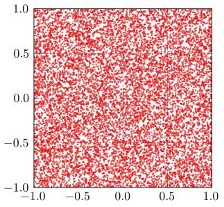
The source function $f(x)$ and the Dirichlet boundary condition $g(x)$ are given by the exact solution Eq (52). We take $d=5$ and $k=4$ in Eq (52), and sample 3001 points in $\Omega$ and 100 points in each hyperplane on $\partial\Omega$ as the training set and 200000 points as the test set. The distribution of the residual training points in the first two dimensions is plotted in Fig 19.

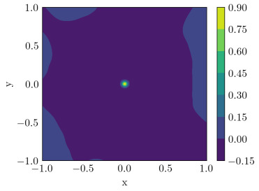
In Figure 20, we compare the numerical results derived from GLP sampling with those from uniform random sampling after 7500 epochs of Adam training and 10000 epochs of LBFGS training. This comparison aims to demonstrate the efficiency of our method for the same number of training points.

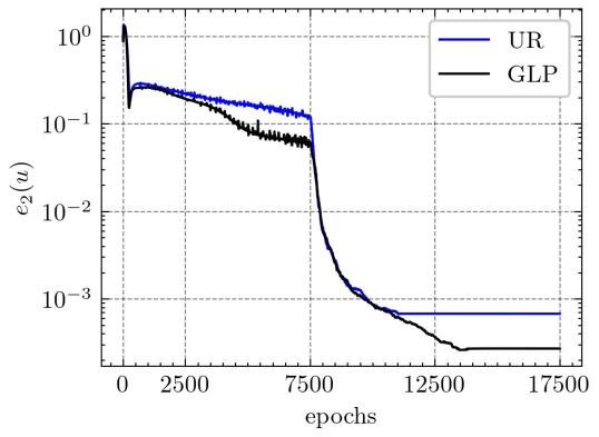
We also developed different training strategies by the number of training points and conducted controlled experiments with the GLP sampling. The results of these different sampling strategies are comprehensively summarized in Table 7. The experimental results conclusively demonstrate that the GLP sampling possesses a clear advantage over uniform random sampling, even when the latter utilizes approximately five times the number of training points.

Table 7: The number of residual points in

\Omega

and the number of boundary points at each hyperplane on

\partial\Omega

using sampling strategies for the five-dimensional nonlinear problem.

Strategy	1	2	3	4
Method	UR	UR	UR	GLP
Residual points	3001	5003	15019	3001
Each hyperplane	100	100	100	100
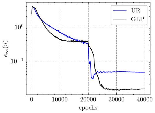
$\bm{e}_{2}(\bm{u})$	$6.813\times 10^{-4}$	$5.075\times 10^{-4}$	$4.027\times 10^{-4}$	$2.728\times 10^{-4}$
$\bm{e}_{\infty}(\bm{u})$	$1.118\times 10^{-2}$	$3.669\times 10^{-3}$	$3.013\times 10^{-3}$	$1.818\times 10^{-3}$

Next, we take $d=8$ and $k=3$ in Eq (52), and sample 11215 points in $\Omega$ and 200 points in each hyperplane on $\partial\Omega$ as the training set and 500000 points as the test set. Moreover, we adjust the weights in the loss function so that $\alpha_{1}=10$ and $\alpha_{2}=1$ . The other settings of main parameters in PINNs are the same as before.The distribution of the residual training points in the first two dimensions is plotted in Fig 21.

In Figure 22, we compare the numerical results derived from GLP sampling with those from uniform random sampling after 20000 epochs of Adam training and 20000 epochs of LBFGS training. This comparison aims to show the effectiveness of our method for the same number of training points. We also developed different training strategies by the number of training points and conducted controlled experiments with the GLP sampling. The results of these different sampling strategies are comprehensively summarized in Table 8. The experimental results conclusively demonstrate that our method is effective.

Table 8: The number of residual points in

\Omega

and the number of boundary points at each hyperplane on

\partial\Omega

using sampling strategies for the eight-dimensional nonlinear problem.

Strategy	1	2	3	4
Method	UR	UR	UR	GLP
Residual points	11215	24041	46213	11215
Each hyperplane	100	100	100	100
$\bm{e}_{2}(\bm{u})$	$1.020\times 10^{-3}$	$8.209\times 10^{-3}$	$5.680\times 10^{-3}$	$4.965\times 10^{-3}$
$\bm{e}_{\infty}(\bm{u})$	$4.702\times 10^{-2}$	$4.330\times 10^{-2}$	$4.251\times 10^{-2}$	$1.512\times 10^{-3}$

5 Conclusions

In this work, we propose a number-theoretic method sampling neural network for solving PDEs, which using a good lattice point (GLP) set as sampling points to approximate the empirical residual loss function of physics-informed neural networks (PINNs), with the aim of reducing estimation errors. From a theoretical perspective, we give the upper bound of the error for PINNs based on the GLP sampling. Additionally, we demonstrate that when using GLP sampling, the upper bound of the expectation of the squared $L_{2}$ error of PINNs is smaller compared to using uniform random sampling. Numerical results based on our method, when addressing low-regularity and high-dimensional problems, indicate that GLP sampling outperforms traditional uniform random sampling in both accuracy and efficiency. In the future, we will work on how to use GLP sampling on other deep learning solvers and how to use number theoretic methods for non-uniform adaptive sampling.

Acknowledgment

This research is partially sponsored by the National Key R & D Program of China (No.2022YFE03040002) and the National Natural Science Foundation of China (No.12371434).

Additionally, we would also like to express our gratitude to Professor KaiTai Fang and Dr. Ping He from BNU-HKBU United International College for their valuable discussions and supports in this research.

Data Availability Statement

The data that support the findings of this study are available from the corresponding author upon reasonable request.

Conflict of Interest

The authors have no conflicts to disclose.

Appendix A

Proof of Theorem 2.

According to the proof of Theorem 1, we recall Eq (26),

\displaystyle\mathbb{E}\left(\mathcal{L}_{N}(\bm{x};\theta_{i+1})\right)\leq(1-c\mu\eta_{i})\mathbb{E}\left(\mathcal{L}_{N}(\bm{x};\theta_{i})\right)+\frac{\eta_{i}^{2}}{2}\mathbf{L}C_{V}s(N_{r},N_{b}).

(53)

Now we will prove this theorem by induction. When $i=1$ , due to the definition of $\kappa$ , it is easy to prove that $\mathbb{E}\left(\mathcal{L}_{N}(\bm{x};\theta_{1})\right)\leq\frac{\kappa}{\xi+1}s(N_{r},N_{b})$ . Assume that when $i=k>1$ , Eq (29) still holds. Next, we consider the case when $i=k+1$ .

According to Eq (53), we have

$\displaystyle\mathbb{E}\left(\mathcal{L}_{N}(\bm{x};\theta_{k+1})\right)$	$\displaystyle\leq(1-c\mu\eta_{k})\frac{\kappa}{\xi+k}s(N_{r},N_{b})+\frac{1}{2}\eta^{2}_{k}\mathbf{L}C_{V}s(N_{r},N_{b})$	(54)
	$\displaystyle=(1-\frac{\beta c\mu}{\xi+k})\frac{\kappa}{\xi+k}s(N_{r},N_{b})+\frac{\beta^{2}\mathbf{L}C_{V}R(N_{r},N_{b})}{2(\xi+k)^{2}}$
	$\displaystyle=\frac{\xi+k-\beta c\mu}{(\xi+k)^{2}}\kappa s(N_{r},N_{b})+\frac{\beta^{2}\mathbf{L}C_{V}R(N_{r},N_{b})}{2(\xi+k)^{2}}$
	$\displaystyle=\frac{\xi+k-1}{(\xi+k)^{2}}\kappa s(N_{r},N_{b})-\frac{\beta c\mu-1}{(\xi+k)^{2}}\kappa s(N_{r},N_{b})+\frac{\beta^{2}\mathbf{L}C_{V}R(N_{r},N_{b})}{2(\xi+k)^{2}}.$

Due to the definition of $\kappa$ , it is observed that $\kappa\geq\frac{\beta^{2}\mathbf{L}C_{V}}{2(\beta c\mu-1)}$ , then we have

\frac{\beta^{2}\mathbf{L}C_{V}R(N_{r},N_{b})}{2(\xi+k)^{2}}-\frac{\beta c\mu-1}{(\xi+k)^{2}}\kappa s(N_{r},N_{b})\leq 0.

(55)

Using Eq (54), there is

$\displaystyle\mathbb{E}\left(\mathcal{L}_{N}(\bm{x};\theta_{k+1})\right)$	$\displaystyle\leq\frac{\xi+k-1}{(\xi+k)^{2}}\kappa s(N_{r},N_{b})-\frac{\beta c\mu-1}{(\xi+k)^{2}}\kappa s(N_{r},N_{b})+\frac{\beta^{2}\mathbf{L}C_{V}R(N_{r},N_{b})}{2(\xi+k)^{2}}$	(56)
	$\displaystyle\leq\frac{\xi+k-1}{(\xi+k)^{2}}\kappa s(N_{r},N_{b})$
	$\displaystyle\leq\frac{\xi+k-1}{(\xi+k)^{2}-1}\kappa s(N_{r},N_{b})$
	$\displaystyle=\frac{\kappa}{\xi+k+1}s(N_{r},N_{b}).$

By induction, we have proved that Eq (29) holds.

∎

References

Bottou et al. [2018] Bottou, L., Curtis, F.E., Nocedal, J., 2018. Optimization methods for large-scale machine learning. SIAM review 60, 223–311.
Caflisch [1998] Caflisch, R.E., 1998. Monte carlo and quasi-monte carlo methods. Acta numerica 7, 1–49.
Chen et al. [2021] Chen, J., Du, R., Li, P., Lyu, L., 2021. Quasi-monte carlo sampling for solving partial differential equations by deep neural networks. Numerical Mathematics 14, 377–404.
Dick et al. [2013] Dick, J., Kuo, F.Y., Sloan, I.H., 2013. High-dimensional integration: the quasi-monte carlo way. Acta Numerica 22, 133–288.
Fang et al. [2018] Fang, K., Liu, M.Q., Qin, H., Zhou, Y.D., 2018. Theory and application of uniform experimental designs. volume 221. Springer.
Fang and Wang [1993] Fang, K.T., Wang, Y., 1993. Number-theoretic methods in statistics. volume 51. CRC Press.
Fu and Wang [2022] Fu, F., Wang, X., 2022. Convergence analysis of a quasi-monte carlo-based deep learning algorithm for solving partial differential equations. arXiv preprint arXiv:2210.16196 .
Halton [1960] Halton, J.H., 1960. On the efficiency of certain quasi-random sequences of points in evaluating multi-dimensional integrals. Numerische Mathematik 2, 84–90.
Hammersley et al. [1965] Hammersley, J., Handscomb, D., Weiss, G., 1965. Monte carlo methods. Physics Today 18, 55–56.
Han et al. [2018] Han, J., Jentzen, A., Weinan, E., 2018. Solving high-dimensional partial differential equations using deep learning. Proceedings of the National Academy of Sciences 115, 8505–8510.
Hlawka [1961] Hlawka, E., 1961. Funktionen von beschränkter variatiou in der theorie der gleichverteilung. Annali di Matematica Pura ed Applicata 54, 325–333.
Hlawka [1962] Hlawka, E., 1962. Zur angenäherten berechnung mehrfacher integrale. Monatshefte für Mathematik 66, 140–151.
Hua [2012] Hua, L.K., 2012. Applications of number theory to numerical analysis. Springer Science & Business Media.
Jin et al. [2021] Jin, X., Cai, S., Li, H., Karniadakis, G.E., 2021. Nsfnets (navier-stokes flow nets): Physics-informed neural networks for the incompressible navier-stokes equations. Journal of Computational Physics 426, 109951.
Kingma and Ba [2014] Kingma, D.P., Ba, J., 2014. Adam: A method for stochastic optimization. arXiv preprint arXiv:1412.6980 .
Korobov [1959a] Korobov, A., 1959a. The approximate computation of multiple integrals, in: Dokl. Akad. Nauk SSSR, pp. 1207–1210.
Korobov [1959b] Korobov, N., 1959b. The evaluation of multiple integrals by method of optimal coefficients. Vestnik Moskovskogo universiteta 4, 19–25.
Krishnapriyan et al. [2021] Krishnapriyan, A., Gholami, A., Zhe, S., Kirby, R., Mahoney, M.W., 2021. Characterizing possible failure modes in physics-informed neural networks. Advances in neural information processing systems 34, 26548–26560.
Li et al. [2020] Li, Z., Kovachki, N., Azizzadenesheli, K., Liu, B., Bhattacharya, K., Stuart, A., Anandkumar, A., 2020. Fourier neural operator for parametric partial differential equations. arXiv preprint arXiv:2010.08895 .
Liu and Nocedal [1989] Liu, D.C., Nocedal, J., 1989. On the limited memory bfgs method for large scale optimization. Mathematical programming 45, 503–528.
Lu et al. [2019] Lu, L., Jin, P., Karniadakis, G.E., 2019. Deeponet: Learning nonlinear operators for identifying differential equations based on the universal approximation theorem of operators. arXiv preprint arXiv:1910.03193 .
Lu et al. [2021] Lu, L., Meng, X., Mao, Z., Karniadakis, G.E., 2021. Deepxde: A deep learning library for solving differential equations. SIAM review 63, 208–228.
Lyu et al. [2020] Lyu, L., Wu, K., Du, R., Chen, J., 2020. Enforcing exact boundary and initial conditions in the deep mixed residual method. arXiv preprint arXiv:2008.01491 .
Lyu et al. [2022] Lyu, L., Zhang, Z., Chen, M., Chen, J., 2022. Mim: A deep mixed residual method for solving high-order partial differential equations. Journal of Computational Physics 452, 110930.
Matsubara and Yaguchi [2023] Matsubara, T., Yaguchi, T., 2023. Good lattice training: Physics-informed neural networks accelerated by number theory. arXiv preprint arXiv:2307.13869 .
Niederreiter [1977] Niederreiter, H., 1977. Pseudo-random numbers and optimal coefficients. Advances in Mathematics 26, 99–181.
Niederreiter [1992] Niederreiter, H., 1992. Random number generation and quasi-Monte Carlo methods. SIAM.
Raissi et al. [2019] Raissi, M., Perdikaris, P., Karniadakis, G.E., 2019. Physics-informed neural networks: A deep learning framework for solving forward and inverse problems involving nonlinear partial differential equations. Journal of Computational physics 378, 686–707.
Renardy and Rogers [2006] Renardy, M., Rogers, R.C., 2006. An introduction to partial differential equations. volume 13. Springer Science & Business Media.
Shin et al. [2020] Shin, Y., Darbon, J., Karniadakis, G.E., 2020. On the convergence of physics informed neural networks for linear second-order elliptic and parabolic type pdes. arXiv preprint arXiv:2004.01806 .
Sirignano and Spiliopoulos [2018] Sirignano, J., Spiliopoulos, K., 2018. Dgm: A deep learning algorithm for solving partial differential equations. Journal of computational physics 375, 1339–1364.
Sobol [1967] Sobol, I., 1967. On the distribution of points in a cube and the approximate evaluation of integrals. USSR Computational Mathematics and Mathematical Physics 7, 86–112.
Stein [1987] Stein, M., 1987. Large sample properties of simulations using latin hypercube sampling. Technometrics , 143–151.
Tang et al. [2020] Tang, K., Wan, X., Liao, Q., 2020. Deep density estimation via invertible block-triangular mapping. Theoretical and Applied Mechanics Letters 10, 143–148.
Tang et al. [2023] Tang, K., Wan, X., Yang, C., 2023. Das-pinns: A deep adaptive sampling method for solving high-dimensional partial differential equations. Journal of Computational Physics 476, 111868.
Weinan and Yu [2018] Weinan, E., Yu, B., 2018. The deep ritz method: A deep learning-based numerical algorithm for solving variational problems. Communications in Mathematics and Statistics 6, 1–12.
Wu et al. [2023] Wu, C., Zhu, M., Tan, Q., Kartha, Y., Lu, L., 2023. A comprehensive study of non-adaptive and residual-based adaptive sampling for physics-informed neural networks. Computer Methods in Applied Mechanics and Engineering 403, 115671.
Yang et al. [2024] Yang, Y., Yang, Q., Deng, Y., He, Q., 2024. Moving sampling physics-informed neural networks induced by moving mesh pde. Neural Networks , 106706.

$\displaystyle\mathcal{L}_{r}(\bm{x};\theta)$	$\displaystyle=\int_{\Omega}\|r(\bm{x};\theta)\|^{2}d\bm{x}=V(\Omega)\int_{\Omega}\|r(\bm{x};\theta)\|^{2}U(\Omega)d\bm{x}$	(3)
	$\displaystyle=V(\Omega)\mathbb{E}_{\bm{x}\sim U}(\|r(\bm{x};\theta)\|^{2})$
	$\displaystyle\approx V(\Omega)\frac{1}{N_{r}}\sum_{i=1}^{N_{r}}\|r(x_{i};\theta)\|^{2},\quad\bm{x}\sim U(\Omega),$

	$\displaystyle\mathbb{E}_{x_{i}}\left(\\|g(x_{i},\theta_{i})\\|_{2}^{2}\right)$	$\displaystyle=\mathbb{V}_{x_{i}}\left(g(x_{i},\theta_{i})\right)+\\|\mathbb{E}_{x_{i}}\left(g(x_{i},\theta_{i})\right)\\|_{2}^{2}$		(22)
		$\displaystyle\leq C_{V}s(N_{r},N_{b})+\left(M_{V}+\mu^{2}_{G}(1+s(N_{r},N_{b}))\right)(1+s(N_{r},N_{b}))\\|\nabla\mathcal{L}_{N}(\bm{x};\theta_{i})\\|_{2}^{2}.$		(22)

		$\displaystyle\mathbb{E}_{x_{i}}\left(\mathcal{L}_{N}(\bm{x};\theta_{i+1})\right)-\mathcal{L}_{N}(\bm{x};\theta_{i})\leq\frac{\eta^{2}}{2}\mathbf{L}\mathbb{E}_{x_{i}}\left(\\|g(x_{i},\theta_{i})\\|_{2}^{2}\right)-\eta\nabla\mathcal{L}_{N}(\bm{x};\theta_{i})^{T}\mathbb{E}_{x_{i}}\left(g(x_{i};\theta_{i})\right)$		(23)
		$\displaystyle\leq\frac{\eta^{2}}{2}\mathbf{L}C_{V}s(N_{r},N_{b})+\frac{\eta^{2}}{2}\mathbf{L}\left(M_{V}+\mu^{2}_{G}(1+s(N_{r},N_{b}))\right)(1+s(N_{r},N_{b}))\\|\nabla\mathcal{L}_{N}(\bm{x};\theta_{i})\\|_{2}^{2}$
		$\displaystyle-\eta\mu(1+s(N_{r},N_{b}))\\|\nabla\mathcal{L}_{N}(\bm{x};\theta_{i})\\|_{2}^{2}$
		$\displaystyle=\frac{\eta^{2}}{2}\mathbf{L}C_{V}s(N_{r},N_{b})-(\eta\mu-\frac{\eta^{2}}{2}\mathbf{L}\left(M_{V}+\mu^{2}_{G}(1+s(N_{r},N_{b}))\right))(1+s(N_{r},N_{b}))\\|\nabla\mathcal{L}_{N}(\bm{x};\theta_{i})\\|_{2}^{2}.$

$\displaystyle C_{1}\\|\bm{u}^{*}(\bm{x})-\bm{u}(\bm{x};\theta)\\|_{2}$	$\displaystyle\leq\\|\mathcal{A}[\bm{u}^{}(\bm{x})]-\mathcal{A}[\bm{u}(\bm{x};\theta)]\\|_{2}+\\|\mathcal{B}[\bm{u}^{}(\bm{x})]-\mathcal{B}[\bm{u}(\bm{x};\theta)]\\|_{2}$	(33)
	$\displaystyle=\\|\mathcal{A}[\bm{u}(\bm{x};\theta)]-f(\bm{x})\\|_{2}+\\|\mathcal{B}[\bm{u}(\bm{x};\theta)]-g(\bm{x})\\|_{2}$
	$\displaystyle=\\|r(\bm{x};\theta)\\|_{2}+\\|b(\bm{x};\theta)\\|_{2}$
	$\displaystyle\leq\sqrt{2}\left(\\|r(\bm{x};\theta)\\|_{2}^{2}+\\|b(\bm{x};\theta)\\|_{2}^{2}\right)^{\frac{1}{2}}.$