A Numerical Verification Framework for Differential Privacy in Estimation

Yunhai Han^1,2 and Sonia Martínez¹ ¹Department of Mechanical and Aerospace Engineering, University of California at San Diego, La Jolla, CA, 92093, USA (email: y8han@ucsd.edu; soniamd@ucsd.edu).²Laboratory for Intelligent Decision and Autonomous Robots, George W. Woodruff School of Mechanical Engineering, Georgia Institute of Technology, Atlanta, GA, 30313, USA (email: yhan364@gatech.edu). This work was supported by Grant ONR N00014-19-1-2471.

Abstract

This work proposes an algorithmic method to verify differential privacy for estimation mechanisms with performance guarantees. Differential privacy makes it hard to distinguish outputs of a mechanism produced by adjacent inputs. While obtaining theoretical conditions that guarantee differential privacy may be possible, evaluating these conditions in practice can be hard. This is especially true for estimation mechanisms that take values in continuous spaces, as this requires checking for an infinite set of inequalities. Instead, our verification approach consists of testing the differential privacy condition for a suitably chosen finite collection of events at the expense of some information loss. More precisely, our data-driven, test framework for continuous range mechanisms first finds a highly-likely, compact event set, as well as a partition of this event, and then evaluates differential privacy wrt this partition. This results into a type of differential privacy with high confidence, which we are able to quantify precisely. This approach is then used to evaluate the differential-privacy properties of the recently proposed $W_{2}$ Moving Horizon Estimator. We confirm its properties, while comparing its performance with alternative approaches in simulation.

I INTRODUCTION

A growing number of emerging, on-demand applications, require data from users or sensors in order to make predictions and/or recommendations. Examples include smart grids, traffic networks, or home assistive technology. While more accurate information can benefit the quality of service, an important concern is that sharing personalized data may compromise the privacy of its users. This has been demonstrated over Netflix datasets [1], as well as on traffic monitoring systems [2].

Initially proposed from the database literature, Differential Privacy [3] addresses this issue, and has become a standard in privacy specification of commercial products. More recently, differential privacy has attracted the attention of the Systems and Control literature [4] and been applied on control systems [5], optimization [6], and estimation and filtering [7]. In particular, the work [8] develops the concept of differential privacy for Kalman filter design. The work [9] proposes a more general moving-horizon estimator via a perturbed objective function to enable privacy. To the best of our knowledge, all of these works only propose sufficient and theoretical conditions for differential privacy.

However, the design of such algorithms can be subtle and error-prone. It has been proved that a number of algorithms in the database literature are incorrect [10] [11], and their claimed level of privacy can not be achieved. Motivated by this, the work [12] introduces an approach to detect the violation of differential privacy for discrete mechanisms. Yet, this method is only applicable for mechanisms that result in a small and finite number of events. Further, a precise characterization of its performance guarantees is not provided.

This motivates our work with contributions in two directions. First, we build a tractable, data-driven, framework to detect violations of differential privacy in system estimation. To handle the infinite collection of events of continuous spaces, the evaluation is conditioned over a highly-likely, compact set. This results into a type of approximate differential privacy with high confidence. We then approximate this set in a data-driven fashion. Further, tests are performed wrt a collectively-exhaustive and mutually exclusive partition of the approximated highly-likely set. By assuming the probability of these events is upper bounded by a small constant, and implementing an exact hypothesis test procedure, we are able to quantify the approximate differential privacy of the estimation wrt two adjacent inputs with high-likelihood. Second, we employ this procedure to evaluate the differential privacy of a previously proposed, $W_{2}$ -MHE estimator. Our experiments show some interesting results including: i) the theoretical conditions for the $W_{2}$ -MHE seem to hold but may be rather conservative, ii) there is an indication that perturbing the output estimation mapping results in a better performance than perturbing the input sensor data, iii) differential privacy does depend on sensor locations, and iv) the $W_{2}$ -MHE performs better than a differentially-private EKF.

II Problem Formulation

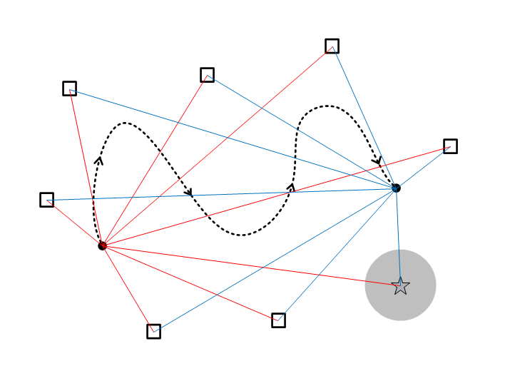
Consider a sensor network performing a distributed estimation task. Sensors may have different owners, who wish to maintain their locations private. Even if communication among sensors is secure, an adversary may have access to the estimation on the target, and other network side information¹¹1This can be any information including, but not limited to, the target’s true location, and all other sensor positions. to gain critical knowledge about any individual sensor; see Figure 1.

Refer to caption — Figure 1: The solid circle represents the moving target that is being estimated; the squares represent the location of known sensors (side information known by an adversary); the star represents the sensor location of a particular sensor that an adversary is tracking. The actual location of the starred sensor can be anywhere within the shaded circle (hypothesis). The diameter of the hypothesis depends on the level of differential privacy of the estimator. The dashed curve represents the target’s trajectory and the arrows indicate the direction. The set of red/blue lines represent the output data released from sensors when the target is at the start/end point. In practice, an adversary can probably have access to a time history of data.

We now start by defining the concept of differential privacy in estimation, and state our problem objectives.

Let a system and observation models be of the form :

\Omega:\begin{cases}x_{k+1}=f\left(x_{k},w_{k}\right),\\ {\color[rgb]{0,0,0}\definecolor[named]{pgfstrokecolor}{rgb}{0,0,0}\pgfsys@color@gray@stroke{0}\pgfsys@color@gray@fill{0}y_{k}=h\left(x_{k},v_{k}\right)},\end{cases}

(1)

where $x_{k}\in\mathbb{R}^{d_{X}},y_{k}\in\mathbb{R}^{d_{Y}}$ , $w_{k}\in\mathbb{R}^{d_{W}}$ and $v_{k}\in\mathbb{R}^{d_{V}}$ . Here, $w_{k}$ and $v_{k}$ represent the iid process and measurement noises at time step $k$ , respectively.

Let $\{0,\ldots,T\}$ be a time horizon, and the sensor data up to time $T$ be denoted by $\mathrm{y}_{0:T}$ $=\left(y_{0}^{\top},\ldots,y_{T}^{\top}\right)^{\top}$ . An estimator or mechanism $\mathcal{M}$ of (1) is a stochastic mapping: ${}^{(T+1)d_{Y}}\rightarrow{}^{md_{X}}$ , for some $m\geq 1$ , which assigns sensor data $\mathrm{y}_{0:T}$ to a random state trajectory estimate. We will assume that the distribution of $\mathcal{M}(\mathrm{y}_{0:T})$ , $\mathbb{P}$ , is independent of the distribution of $\mathrm{y}_{0:T}$ . In Section V, we test a $W_{2}$ -MHE filter that takes this form and assimilates sensor data online. Roughly speaking, the $W_{2}$ -MHE employs a moving window $N$ and sensor data $(y_{k+1},\ldots,y_{k+N})$ to estimate the state at time $k$ ; see [9] for more information.

Definition 1

(( $\varepsilon$ , $d$ -adjacent), $\lambda$ -approximate, Differential Privacy) Let $\mathcal{M}$ be a state estimator of System 1 and $d_{\mathrm{y}}$ a distance metric on ${}^{(T+1)d_{Y}}$ . Given $\varepsilon,\lambda,d\in\mathbb{R}_{\geq 0}$ , $\mathcal{M}$ is ( $\varepsilon$ , $d$ -adjacent), $\lambda$ -approximate, differentially private if for any $\mathrm{y}_{0:T}^{1},\mathrm{y}_{0:T}^{2}\in{}^{(T+1)d_{Y}}$ , with $d_{\mathrm{y}}(\mathrm{y}_{0:T}^{1},\mathrm{y}_{0:T}^{2})\leq d$ we have

{\small\mathbb{P}(\mathcal{M}\left(\mathrm{y}_{0:T}^{i})\in E\right)\leq\mathrm{e}^{\varepsilon}{\mathbb{P}(\mathcal{M}(\mathrm{y}_{0:T}^{j})\in E))}+\lambda,\;}

(2)

for $i,j=1,2,$ and for all $E\subset\text{range}(\mathcal{M})$ . In what follows, we use the notation $(\varepsilon,d$ -adj $)$ - $\lambda$ (resp. $(\varepsilon,d$ -adj $)$ , for $\lambda=0$ ).

This notion of privacy matches the standard definition of [4][8], for a $1$ -adjacency relation given by a distance $\leq d$ . We are mostly interested in the case of $\lambda=0$ and the standard $(\varepsilon,d$ -adj $)$ differential privacy [9]. However, later we discuss how to choose a $\lambda$ to approximate it via $(\varepsilon,d$ -adj $)$ - $\lambda$ differential privacy. Ideally, $\lambda$ is to be chosen as small as possible. Here, $d_{\mathrm{y}}\left(\mathrm{y}_{0:T}^{1},\mathrm{y}_{0:T}^{2}\right)$ is induced by the 2-norm. However, the results do not depend on the choice of metric.

Finding theoretical conditions that guarantee $(\varepsilon$ , $d$ -adj $)$ differential privacy can be difficult, conservative, and hard to verify. Thus, in this work we aim to:

1.

Obtain a tractable, numerical test procedure to evaluate the differential privacy of an estimator; while providing quantifiable performance guarantees of its correctness.
2.

Verify numerically the differential-privacy guarantees of the $W_{2}$ -MHE filter of [9]; and compare its performance with that of an extended Kalman filter.
3.

Evaluate the differences in privacy/estimation when the perturbations are directly applied to the sensor data before the filtering process is done.

Our approach employs a statistical, data-driven method. Although a main motivation for this work is the evaluation of the $W_{2}$ -MHE filter, the method can be used to verify the privacy of any mappings with a continuous space range.

III Approximate $(\varepsilon$ , $d$ -adj $)$ Differential Privacy

In this section, we start by introducing a notion of high-likelihood $(\varepsilon$ , $d$ -adj $)$ differential privacy. This is a first step to simplify the evaluation of differential privacy via the proposed numerical framework. A second step lies on the identification of a suitable space partition.

Definition 2

(High-likelihood $(\varepsilon$ , $d$ -adj $)$ Differential Privacy). Suppose that $\mathcal{M}$ is a state estimator of System 1. Given $\varepsilon,d\in{\color[rgb]{0,0,0}\definecolor[named]{pgfstrokecolor}{rgb}{0,0,0}\pgfsys@color@gray@stroke{0}\pgfsys@color@gray@fill{0}\mathbb{R}_{\geq 0}}$ , we say that $\mathcal{M}$ is $(\varepsilon$ , $d$ -adj $)$ differentially private with high likelihood $1-\theta$ if there exists an event $R$ with $\mathbb{P}(R)\geq 1-\theta$ such that, for any two $\mathrm{y}_{0:T}^{i}$ , $i=1,2$ , with $d_{\mathrm{y}}(\mathrm{y}_{0:T}^{1},\mathrm{y}_{0:T}^{2})\leq d$ , we have:

\mathbb{P}(\mathcal{M}(\mathrm{y}_{0:T}^{i})\in E|R)\leq e^{\varepsilon}\mathbb{P}(\mathcal{M}(\mathrm{y}_{0:T}^{j})\in E|R),

for $i,j\in\{1,2\}$ and all events $E\subseteq\text{range}(\mathcal{M})$ .

Lemma 1

Suppose that $\mathcal{M}$ is a high-likelihood $(\varepsilon$ , $d$ -adj $)$ differentially private estimator, with likelihood $1-\theta$ . Then, $\mathcal{M}$ is $(\varepsilon$ , $d$ -adj $)$ - $\lambda$ differentially private with $\lambda=\theta$ .

Proof:

Let $R$ be the high-likely event wrt which $\mathcal{M}$ is high-likely differentially private. Let $\overline{R}$ be its complement and $E\subseteq\text{range}(\mathcal{M})$ . We have

	$\displaystyle\mathbb{P}(\mathcal{M}(\mathrm{y}_{0:T}^{1})\in E)$
	$\displaystyle=\mathbb{P}(\mathcal{M}(\mathrm{y}_{0:T}^{1})\in E\|R)\mathbb{P}(R)+\mathbb{P}(\mathcal{M}(\mathrm{y}_{0:T}^{1})\in E\|\overline{R})\mathbb{P}(\overline{R})$
	$\displaystyle\leq e^{\varepsilon}\mathbb{P}(\mathcal{M}(\mathrm{y}_{0:T}^{2})\in E\|R)\mathbb{P}(R)+\theta\mathbb{P}(\mathcal{M}(\mathrm{y}_{0:T}^{1})\in E\|\overline{R})\leq$
	$\displaystyle e^{\varepsilon}[\mathbb{P}(\mathcal{M}(\mathrm{y}_{0:T}^{2})\in E\|R)\mathbb{P}(R)+\mathbb{P}(\mathcal{M}(\mathrm{y}_{0:T}^{2})\in E\|\overline{R})\mathbb{P}(\overline{R})]+\theta$
	$\displaystyle=e^{\varepsilon}\mathbb{P}(\mathcal{M}(\mathrm{y}_{0:T}^{2})\in E)+\theta,$

similarly, the roles of $\mathrm{y}_{0:T}^{1}$ and $\mathrm{y}_{0:T}^{2}$ can be exchanged. ∎

Definition 2 still requires checking conditions involving an infinite number of event sets. Our test framework limits evaluations to a finite collection as follows.

Definition 3 (Differential privacy wrt a space partition)

Let $\mathcal{M}$ be an estimator of System 1 and $\mathcal{P}=\{E_{1},\ldots,E_{n}\}$ be a space partition²²2By partition we mean a collection of mutually exclusive and collectively exhaustive set of events wrt $\mathbb{P}$ . of $\text{range}(\mathcal{M})$ . We say that $\mathcal{M}$ is $(\varepsilon$ , $d$ -adj $)$ differentially private wrt $\mathcal{P}$ if the definition of $(\varepsilon$ , $d$ -adj $)$ differential privacy holds for each $E_{k}\in\mathcal{P}$ .

The following helps explain the relationship between $(\varepsilon$ , $d$ -adj $)$ differential privacy wrt a partition and the original $(\varepsilon$ , $d$ -adj $)$ differential privacy.

Lemma 2

Let $\mathcal{M}$ be a state estimator of System 1, and consider a partition of $\text{range}(\mathcal{M})$ , $\mathcal{P}_{1}=\{E_{1},\ldots,E_{n_{1}}\}$ , which is finer than another partition $\mathcal{P}_{2}$ $=\{F_{1},\ldots,F_{n_{2}}\}$ ( $n_{1}>n_{2}$ ). That is, each $F_{i}$ can be represented by the disjoint union $F_{i}=\operatorname{\cup}_{s=1}^{m_{i}}E_{l_{s}}$ . Then, if $\mathcal{M}$ is $(\varepsilon$ , $d$ -adj $)$ differentally private wrt $\mathcal{P}_{1}$ , then it is also differentially private wrt $\mathcal{P}_{2}$ .

Proof:

By assumption, it holds that $\mathbb{P}\left(\mathcal{M}\left(\mathrm{y}_{0:T}^{1}\right)\in E_{i}\right)$ $\leq\mathrm{e}^{\varepsilon}\mathbb{P}\left(\mathcal{M}\left(\mathrm{y}_{0:T}^{2}\right)\in E_{i}\right)$ . Take $F_{i}=E_{l_{1}}\operatorname{\cup}\ldots\operatorname{\cup}E_{l_{m_{i}}}$ , then, from the properties of partition, we obtain:

\begin{array}[]{ll}&\mathbb{P}\left(\mathcal{M}\left(\mathrm{y}_{0:T}^{1}\right)\in F_{i}\right)=\mathbb{P}\left(\mathcal{M}\left(\mathrm{y}_{0:T}^{1}\right)\in E_{l_{1}}\operatorname{\cup}\ldots\operatorname{\cup}E_{l_{m_{i}}}\right)\\ &=\sum^{m_{i}}_{s=1}\mathbb{P}\left(\mathcal{M}\left(\mathrm{y}_{0:T}^{1}\right)\in E_{l_{s}}\right)\\ &\leq e^{\varepsilon}\sum^{m_{i}}_{s=1}\mathbb{P}\left(\mathcal{M}\left(\mathrm{y}_{0:T}^{2}\right)\in E_{l_{s}}\right)=e^{\varepsilon}\mathbb{P}\left(\mathcal{M}\left(\mathrm{y}_{0:T}^{2}\right)\in F_{i}\right).\end{array}

Similarly, the roles of $\mathrm{y}_{0:T}^{1}$ and $\mathrm{y}_{0:T}^{2}$ can be exchanged.∎

Thus, it follows intuitively that $\mathcal{M}$ is $(\varepsilon$ , $d$ -adj $)$ differentially private if it is $(\varepsilon$ , $d$ -adj $)$ differentially private wrt infinitesimally small partitions. Now, by considering partitions of a given resolution, we can also guarantee a type of approximate $(\varepsilon$ , $d$ -adj $)$ privacy:

Lemma 3

Consider a partition $\mathcal{P}=\{E_{i}\}_{i\in\mathcal{I}}$ such that $\mathbb{P}(E_{i})\leq\eta$ for all $i\in\mathcal{I}$ . Then, if $(\varepsilon$ , $d$ -adj $)$ differential privacy holds wrt the partition $\mathcal{P}$ , then $\mathcal{M}$ is $(\varepsilon$ , $d$ -adj $)$ - $\lambda$ differentially private with $\lambda=2\eta e^{\varepsilon}$ .

Proof:

For any $R$ , we have $\mathbb{P}(\mathcal{M}(\mathrm{y}_{0:T}^{1})\in R)=\sum_{i}\mathbb{P}(\mathcal{M}(\mathrm{y}_{0:T}^{1})\in R\cap E_{i}).$ By hypothesis,

	$\displaystyle\mathbb{P}(\mathcal{M}(\mathrm{y}_{0:T}^{1})\in E_{i})\leq e^{\varepsilon}\mathbb{P}(\mathcal{M}(\mathrm{y}_{0:T}^{2})\in E_{i})\Longleftrightarrow$
	$\displaystyle\mathbb{P}(\mathcal{M}(\mathrm{y}_{0:T}^{1})\in E_{i}\cap(R\cup\overline{R}))\leq e^{\varepsilon}\mathbb{P}(\mathcal{M}(\mathrm{y}_{0:T}^{2})\in E_{i}\cap(R\cup\overline{R})),$

for $i\in\mathcal{I}$ , and where $\overline{R}$ is the complement of $R$ . Thus,

	$\displaystyle\mathbb{P}(\mathcal{M}(\mathrm{y}_{0:T}^{1})\in E_{i}\cap R)+\mathbb{P}(\mathcal{M}(\mathrm{y}_{0:T}^{1})\in E_{i}\cap\overline{R})$
	$\displaystyle\leq e^{\varepsilon}\mathbb{P}(\mathcal{M}(\mathrm{y}_{0:T}^{2})\in E_{i}\cap R)+e^{\varepsilon}\mathbb{P}(\mathcal{M}(\mathrm{y}_{0:T}^{2})\in E_{i}\cap\overline{R}).$

Now, if $\mathbb{P}(E_{i})\leq\eta$ , we have

\displaystyle\mathbb{P}(\mathcal{M}(\mathrm{y}_{0:T}^{1})\in E_{i}\cap R)\leq e^{\varepsilon}\mathbb{P}(\mathcal{M}(\mathrm{y}_{0:T}^{2})\in E_{i}\cap R)+2\eta e^{\varepsilon}.

Similarly, the roles of $\mathrm{y}_{0:T}^{1},\mathrm{y}_{0:T}^{2}$ can be exchanged. ∎

Our approach is based on checking differential privacy wrt a partition given by $\{\overline{R},E_{i}\}_{i=1}^{n}$ , where $\overline{R}$ is the complement of a highly likely event, and $\{E_{i}\}$ is a partition of $R$ .

IV Differential Privacy Test Framework

In this section, we present the components of our test framework (Section IV-A) and its theoretical guarantees (Section IV-B).

IV-A Overview of the differential-privacy test framework

Privacy is evaluated wrt two $d$ -close $\mathrm{y}_{0:T}^{1}$ , $\mathrm{y}_{0:T}^{2}$ as follows:

1.

Instead of verifying $(\varepsilon$ , $d$ -adj $)$ privacy for an infinite number of events, an EventListGenerator module extracts a finite collection EventList. This is done by partitioning an approximated high-likely event set.
2.

Next, a WorstEventSelector module identifies the worst-case event in EventList that violates $(\varepsilon$ , $d$ -adj $)$ differential privacy with the highest probability.
3.

Finally, a HypothesisTest module evaluates $(\varepsilon$ , $d$ -adj $)$ ifferential privacy wrt the worst-case event.

The overall description is summarized in Algorithm 1.

1:function Test Framework(

\mathcal{M},\varepsilon

\mathrm{y}_{0:T}^{1},\mathrm{y}_{0:T}^{2}

)

2: Inputs: Target estimator

\mathcal{M}

, privacy level

\varepsilon

, sensor data (

\mathrm{y}_{0:T}^{1},\mathrm{y}_{0:T}^{2}

)

3: EventList = EventListGenerator(

\mathcal{M}

\mathrm{y}_{0:T}^{1}

)

4: WorstEvent =

5: WorstEventSelector(

\mathcal{M},\varepsilon,\mathrm{y}_{0:T}^{1},\mathrm{y}_{0:T}^{2}

6: EventList)

p^{+},p_{+}

= HypothesisTest(

\mathcal{M},\varepsilon

\mathrm{y}_{0:T}^{1},\mathrm{y}_{0:T}^{2}

8: WorstEvent)

9: Return

p^{+},p_{+}

10:end function

Algorithm 1

(\varepsilon

d

-adj

)

Differentially-private Test Framework

We now describe each module in detail.

IV-A1 EventListGenerator module.

Consider System 1, with initial condition $x_{0}\in\mathcal{K}_{0}\subset\mathbb{R}^{d_{X}}$ . The estimated state $\hat{x}_{k}$ under $\mathcal{M}$ for a given $\mathrm{y}_{0:T}^{1}$ , belongs to a set of all possible estimates given $x_{0}$ and $\mathrm{y}_{0:T}^{1}$ . Denote this set as $R_{[0,k]}$ .

In [9], this set is bounded as all disturbances and initial distribution are assumed to have a compact support. However, $R_{[0,k]}$ can be unbounded for other estimators. To reduce the set of events to be checked for $(\varepsilon$ , $d$ -adj $)$ differential privacy: a) we approximate the set $R_{[0,k]}$ by a compact, high-likely set in a data-driven fashion, and b) we finitely partition this set by a mutually exclusive collection of events; see Algorithm 2.

1:function EventListGenerator(

\mathcal{M}

\mathrm{y}_{0:T}^{1}

\beta,\gamma

)

2: Input: Target Estimator(

\mathcal{M}

)

3: In put: Sensor Data(

\mathrm{y}_{0:T}^{1}

)

4: In put: Parameters for Algorithm 3 (

\beta,\gamma

)

5: HighLikelySet

\leftarrow

Apply Algorithm 3

6: EventList

\leftarrow

a partition of the HighLikelySet

7: Return EventList

8:end function

Algorithm 2 EventListGenerator

Inspired by [13] focusing on reachability, we employ the Scenario Optimation approach to approximate a high-likely set via a product of ellipsoids; see Algorithm 3. Here, $\Gamma\equiv\Gamma(\beta)$ defines the number of estimate samples (filter runs) required to guarantee that the output set contains $1-\beta$ of the probability mass of $R_{[0,k]}$ with high confidence $1-\gamma$ . Then, a convex optimization problem is solved to find the output set as a hyper-ellipsoid with parameters $A^{k}$ and $b^{k}$ .

1:Input: Target Estimator(

\mathcal{M}

) with dimension

d_{X}

2:In put: Sensor data(

\mathrm{y}_{0:T}^{1}

), parameters

\beta,\gamma

3:Output: Matrix

A^{k}

and vector

b^{k}

representing an

4:Ou tput:

1

\beta

-accurate high-likely set at time step

k

5:Ou tput:

R_{k}(A^{k},b^{k})=\left\{x\in{}^{d_{X}}\,|\,\|A^{k}x+b^{k}\|_{2}\leq 1\right\}

6:Ou tput: with confidence

1-\gamma

7:Set number of samples

\Gamma

8:Ou tput:

\left[\frac{1}{\beta}\frac{e}{e-1}\left(\log\frac{1}{\gamma}+d_{X}(d_{X}+1)/2+d_{X}\right)\right\rceil

9:for

k\in\{0,\ldots,T\}

10: for

i\in\{0,\ldots,\Gamma\}

11: Record

z^{k}_{i}

\mathcal{M}\left(\mathrm{y}_{0:k}^{1}\right)

12: end for

13: Solve the convex problem

14:

\begin{array}[]{ll}\arg\min_{A^{k},b^{k}}&-\log\operatorname{det}A^{k}\\ \text{subject to }&\left\|A^{k}z^{k}_{i}-b^{k}\right\|_{2}-1\leq 0,\,i=0,\ldots,\Gamma\end{array}

15: return

A^{k},b^{k}

16:end for

Algorithm 3 HighLikelySet

The data-driven approximation of the high-likely set can now be partitioned using e.g. a grid per time step. This is what we do in simulation later. For the $W_{2}$ -MHE, the last $N$ (window size) steps would not be evaluated for differential privacy. Thus, the high-likely set is the product of $T+1-N$ ellipsoids. Alternatively, an outline on how to re-use the sample runs of Algorithm 3 to find a finite partition of the approximated set with a common upper-bounded probability is provided as follows.

Observe that $\Gamma\equiv\Gamma(\beta)$ is a function of $\beta$ , and denote the output of Algorithm 3 by $R$ . For $\eta>\beta$ , we can choose a number of samples $\Gamma(\eta)<\Gamma(\beta)$ and solve a similar convex problem as in step [13:]. The resulting hyper-ellipsoid, $\overline{E}$ , satisfies $\overline{E}\cap R\neq\emptyset$ as they contain common sample runs, and $\mathbb{P}(\overline{E}\cap R)=\mathbb{P}(\overline{E})+\mathbb{P}(R)-\mathbb{P}(\overline{E}\cup R)\geq 1-\eta+1-\beta-1=1-\eta-\beta$ with confidence $1-\gamma$ . Similarly, the complement of $\overline{E}$ , $E$ , is such that $E\cap R\neq\emptyset$ and $\mathbb{P}(E\cap R)=\mathbb{P}(R)-\mathbb{P}(R\cap\overline{E})\leq 1-(1-\eta-\beta)=\eta+\beta$ . This process can be repeated by choosing different subsets of sample runs to find a finite collection of sets $E_{1}\cap R,\dots,E_{n}\cap R$ such that $\mathbb{P}(E_{i}\cap R)\leq\eta+\beta$ and $(E_{1}\cap R)\cup\dots\cup(E_{n}\cap R)=R$ . Wlog, it can be assumed that the sets are mutually exclusive by re-assigning sets overlaps to one of the sets. This approach can be extended to achieve any desired upper bound $\eta_{d}$ for a desired $\beta_{d}$ . To do this, first run Algorithm 3 with respect to $\bar{\beta}$ so that $\eta_{d}>2\bar{\beta}$ . This results into a set $\bar{R}$ with probability at least $1-\bar{\beta}$ and high confidence $1-\gamma$ . By selecting a subset of sample runs $\Gamma(\beta_{d})$ and solving the associated optimization problem, one can obtain $R$ with the desired probability lower-bound $1-\beta_{d}$ . Now, following the previous strategy for $\bar{\eta}=\eta_{d}-\bar{\beta}$ , we can obtain a partition of $R$ and $\bar{R}$ with probability upper bounded by $\bar{\eta}+\bar{\beta}=\eta_{d}$ and high confidence $1-\gamma$ .

We also note that a finite partition of a compact set is always guaranteed to exist under certain conditions, in particular, as the following:

Lemma 4

Let $R$ be a compact set in ^d. If $\mathbb{P}$ is an absolutely continuous measure wrt the Lebesgue measure in ^d, and if the Randon-Nikodym derivative of $\mathbb{P}$ is a continuous function, then there is a finite partition of $R$ of a given resolution $\eta$ .

Proof:

First of all, from absolutely continuity, $\mathbb{P}(E)=\int_{E}fd\mu$ , where $\mu$ is the Lebesgue measure, and $f$ the Randon-Nikodym derivative. Second, observe that we can take arbitrarily small-volume neighborhoods $E_{x}$ , of points of $x\in R$ , to make $\mathbb{P}(E_{x}\cap R)$ as small as we like. This follows from $\mathbb{P}(E_{x}\cap R)\leq\text{vol}(E_{x})\sup_{E_{x}\cap R}f\leq\text{vol}(E_{x})\max_{R}f\leq\eta$ , where $\text{vol}(E_{x})$ is the standard volume of the set $E_{x}$ wrt the Lebesgue measure, and $\max_{R}f<\infty$ by compactness of $R$ and continuity of $f$ . Using these neighborhoods, we can construct an open cover $\{E_{x}\}_{x\in R}$ of $R$ , i.e. $R\subseteq\cup_{x\in R}E_{x}$ . By compactness of $R$ , there must exist a finite subcover $\{E_{1},\dots,E_{n}\}$ , i.e. $R\subseteq E_{1}\cup\dots\cup E_{n}$ . From this cover, we can obtain $\{E_{1}\cap R,\dots,E_{n}\cap R\}$ , with probabilities $\mathbb{P}(E_{i}\cap R)\leq\eta$ , for each $i$ . Now the sets $E_{i}\cap R$ can then be used to construct a finite partition of $R$ , with probabilities that will be less or equal than $\eta$ . ∎

IV-A2 WorstEventSelector module.

We now discuss how to select an $E^{*}$ , a most-likely event that leads to a violation of $(\varepsilon$ , $d$ -adj $)$ differential privacy; see Algorithm 4.

1:function WorstEventSelector(

n,\mathcal{M}

\varepsilon

\mathrm{y}_{0:T}^{1},\mathrm{y}_{0:T}^{2}

, EventList)

2: Input: Target Estimator(

\mathcal{M}

)

3: In put: Desired differential privacy(

\varepsilon

)

4: In put:

d

-adjacent sensor data(

\mathrm{y}_{0:T}^{1},\mathrm{y}_{0:T}^{2}

)

5: In put: EventList

O_{1}

\leftarrow

Estimate set after

n

runs of

\mathcal{M}(\mathrm{y}_{0:T}^{1})

O_{2}

\leftarrow

Estimate set after

n

runs of

\mathcal{M}(\mathrm{y}_{0:T}^{2})

\texttt{\small pvalues}\leftarrow[\phantom{i}]

9: for

E\in

EventList do

10:

c_{1}

\leftarrow

|\{i|O_{1}[i]\in E\}|

11:

c_{2}

\leftarrow

|\{i|O_{2}[i]\in E\}|

12:

p^{+},p_{+}\leftarrow

PVALUE

(c_{1},c_{2},n,\varepsilon)

13:

p^{*}\leftarrow\min{(p^{+},p_{+})}

14: pvalues.append(

p^{*}

)

15: end for

16: WorstEvent

\leftarrow

EventList[

\operatorname{argmin}\{\texttt{\small pvalues}\}

]

17: Return

E^{*}=

WorstEvent

18:end function

Algorithm 4 WorstEvent Selector

The returned WorstEvent ( $E^{*}$ ) is then used in Hypothesis Test function in Algorithm 1. First, WorstEventSelector receives an EventList from EventListGenerator. The algorithm runs the estimator $n$ times with each sensor data, and counts the number of estimates that fall in each event of the list, respectively. Then, a PVALUE function is run to get $p^{+},p_{+}$ ; see Algorithm 5 (top). The $p$ -values quantify the probability of the Type I error of the test (refer to the next subsection).

IV-A3 HypothesisTest module.

The hypothesis test module aims to verify $(\varepsilon$ , $d$ -adj $)$ privacy in a data-driven fashion for a fixed $E^{*}$ . Given a sequence of $m$ statistically-independent trials, the ocurrence or non-occurrence of $\mathcal{M}(\mathrm{y}_{0:T}^{i})\in E$ is a Bernouilli sequence and the number of occurrences in $m$ trials is distributed as a Binomial.

1:function pvalue(

c_{1},c_{2},n,\varepsilon

)

\bar{c_{1}}\leftarrow

c_{1},1/e^{\varepsilon}

)

s\leftarrow\bar{c_{1}}+c_{2}

p^{+}\leftarrow

1 - Hypergeom.cdf(

\bar{c_{1}}-1|2n,n,s

)

\bar{c_{2}}\leftarrow

c_{2},1/e^{\varepsilon}

)

s\leftarrow\bar{c_{2}}+c_{1}

p_{+}\leftarrow

1 - Hypergeom.cdf(

\bar{c_{2}}-1|2n,n,s

)

8: return

p^{+},p_{+}

9:end function

10:function HypothesisTest(

{\color[rgb]{0,0,0}\definecolor[named]{pgfstrokecolor}{rgb}{0,0,0}\pgfsys@color@gray@stroke{0}\pgfsys@color@gray@fill{0}m},\mathcal{M}

\varepsilon

\mathrm{y}_{0:T}^{1},\mathrm{y}_{0:T}^{2}

E^{*}

)

11: Input: Target Estimator(

\mathcal{M}

)

12: In put: Desired differential privacy(

\varepsilon

)

13: In put:

d

-adjacent sensor data(

\mathrm{y}_{0:T}^{1},\mathrm{y}_{0:T}^{2}

)

14: In put:

E^{*}

(WorstEvent)

15:

O_{1}

\leftarrow

Estimate set after

m

runs of

\mathcal{M}(\mathrm{y}_{0:T}^{1})

16:

O_{2}

\leftarrow

Estimate set after

m

runs of

\mathcal{M}(\mathrm{y}_{0:T}^{2})

17:

c_{1}

\leftarrow

|\{i|O_{1}[i]\in E^{*}\}|

18:

c_{2}

\leftarrow

|\{i|O_{2}[i]\in E^{*}\}|

19:

p^{+},p_{+}\leftarrow

PVALUE

(c_{1},c_{2},m,\varepsilon)

20: Return

p^{+},p_{+}

21:end function

Algorithm 5 HypothesisTest

Thus, the verification reduces to evaluating how the parameters of two Binomial distributions differ. More precisely, define $p_{i}=\mathbb{P}\left(\mathcal{M}\left(\mathrm{y}_{0:T}^{i}\right)\in E^{*}\right)$ , $i=1,2$ . By running $m$ times the estimator, we count the number of $\mathcal{M}\left(\mathrm{y}_{0:T}^{i}\right)\in E^{*}$ as $c_{i}$ , $i=1,2$ . Thus, each $c_{i}$ can be seen as a sample of the binomial distribution B $(n_{i},p_{i})$ , for $i=1,2$ . However, instead of evaluating $p_{1}\leq p_{2}$ , we are interested in testing the null hypothesis $p_{1}\leq\mathrm{e}^{\varepsilon}p_{2}$ , with an additional $\mathrm{e}^{\varepsilon}$ . This can be addressed by considering samples $\bar{c}_{1}$ of B( $c_{1},1/e^{\varepsilon}$ ) distribution. It is easy to see the following:

Lemma 5 ([12].)

Let $Y\sim$ B( $n,p_{1}$ ), and $Z$ be sampled from B( $Y,1/e^{\varepsilon}$ ), then, $Z$ is distributed as B( $n,p_{1}/e^{\varepsilon}$ ).

Hence, the problem can be reduced to the problem of testing the null hypothesis $\bar{H}_{0}:\bar{p}_{1}:=p_{1}/e^{\varepsilon}\leq p_{2}$ on the basis of the samples $\bar{c}_{1}$ , $c_{2}$ . Checking whether or not $\bar{c}_{1}$ , $c_{2}$ are generated from the same binomial distribution can be done via a Fisher’s exact test [14] wth $p$ -value being equal to 1 - Hypergeometric.cdf( $\bar{c}_{1}-1|2m,m,\bar{c}_{1}+c_{2}$ ) (cumulative hypergeometric distribution) . As an exact test, $c_{1}\gg e^{\varepsilon}c_{2}$ provides firm evidence against the null hypothesis with a given confidence.

The $p$ -value is the Type I error of the test, or the probability of incorrectly rejecting $H_{0}$ when it is indeed true. The null hypothesis is rejected based on a significance level $\alpha$ (typically $0.1$ , $0.05$ or $0.01$ ). If $p$ is such that $p\leq\alpha$ , then the probability that a mistake is made by rejecting $H_{0}$ is very small (smaller or equal than $\alpha$ ). Since Condition 2 involves two inequalities $p_{1}\leq e^{\varepsilon}p_{2}$ and $p_{2}\leq e^{\varepsilon}p_{1}$ , we need to evaluate two null hypotheses. This results into $p_{+}$ and $p^{+}$ values that should be larger than $\alpha$ if we want to accept $H_{0}$ ; see Algorithm 5. In simulation, we choose $m>n$ in both WorstEventSelector and HypothesisTest for the purpose of i) increasing the accuracy of the test for the worst event, ii) some additional practical considerations as follows.

In the WorstEventSelector, the $p$ -values for all the events are computed using the same $\varepsilon$ , for example, $\varepsilon=1$ . And then the worse event $E^{*}$ which gives the minimum $p$ -value is selected. Later, in HypothesisTest, $c_{1},c_{2}$ are counted with respect to the worse event and then we keep increasing $\varepsilon$ and running PVALUE with the same $c_{1},c_{2}$ until the $p$ -value is larger than $\alpha$ . The critical values are reported in Section . The reasons why we select the same $\varepsilon$ in WorstEventSelector are:

•

The p-value evolves consistently with respect to the test $\varepsilon$ . For example, the event with $c_{1}=12,c_{2}=27$ is the most possible event that shows the violatation of differential privacy. From Figure 2, we can see that no matter what value $\varepsilon$ is chosen, the $p$ -values for that event are the smallest, which means in WorstEventSelector, it will always be returned as the worst event $E^{*}$ . This happens similarly for the event selected from $c_{1}=14,c_{2}=27$ , the $p-$ -values are always the largest. In that case, it is safe to select one specific $\varepsilon$ in WorstEventSelector to decide which event is the worst.

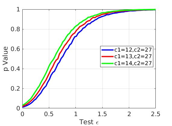
Figure 2: $p$ -values evolution with respect to different choices of event. It is clear that no matter what value $\varepsilon$ is chosen, $p$ -values for the worst event are the smallest.
•

On the other hand, the variations may come from the scenarios that $c_{2}/c_{1}=$ constant, but $(c_{1},c_{2})$ share different values, such as (10,20), (15,30), (20, 40). From Figure 3, for different $\varepsilon$ , the $p$ -values are almost similar. Hence, in this case, in WorstEventSelector, the returned worst event is still the one of the events, if any, that are most likely to show the violations of differential privacy.

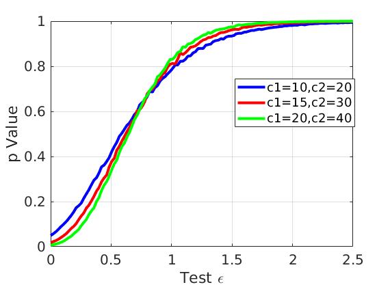
Figure 3: $p$ -values evolution with respect to different choices of event. For different choices of event, the variations are not significant.

IV-B Theoretical Guarantee

Here, we specify the guarantees of the numerical test.

Theorem 1

Let ${\mathcal{M}}$ be a state estimator of System 1, and let $\varepsilon,d,\beta$ and $\gamma\in\mathbb{R}_{\geq 0}$ . We denote two $d$ -adjacent sensor data as $\mathrm{y}_{0:T}^{i}$ , $i\in\{1,2\}$ and a partition of the high-likely ( $1-\beta$ ) set $R$ from Algorithm 3 with high confidence $1-\gamma$ as $\mathcal{P}=\{E_{1},\ldots,E_{n}\}$ such that $\mathbb{P}(E_{i})\leq\eta$ for all $i$ . Then, if $\Gamma$ is selected accordingly, and the estimator passes the test in Algorithm 1, then ${\mathcal{M}}$ is approximately $(\varepsilon$ , $d$ -adj $)$ differentially private wrt $\mathrm{y}_{0:T}^{i}$ , $i\in\{1,2\}$ , and $\lambda=\beta+2\eta\text{e}^{\varepsilon}$ , with confidence $(1-\alpha)(1-\gamma)$ .

Proof:

First, from Scenario Optimization $R$ is a highly likely event ( $1-\beta$ ) with high confidence ( $1-\gamma$ ), and approximate differential privacy with $\lambda=\beta+2\eta e^{\varepsilon}$ is a consequence of the previous lemmas in Section III. Second, as Fisher’s test is exact, the chosen significance level $\alpha$ characterizes exactly the Type I error of the test for any number of samples. If Fisher’s test is applied to the worst-case event in the partition, we can guarantee approximate differential privacy with confidence $1-\gamma$ does not hold with probability $\alpha$ . ∎

To extend the result over any two $d$ -adjacent sensor data, one would have to sample over the measurement space and evaluate the ratio of passing the tests.

V EXPERIMENTS

In this section, we evaluate our test on a toy dynamical system. All simulations are performed in MATLAB (R2020a).

System Example.

Consider a non-isotropic oscillator in ² with potential function $V\left(x^{1},x^{2}\right)=\frac{1}{2}((x^{1})^{2}+4(x^{2})^{2}).$ Thus, the corresponding oscillator particle with position $\mathbf{x}_{k}=(x^{1}_{k},x^{2}_{k})\in{}^{2}$ moves from initial conditions $x^{1}_{0}=5,x^{2}_{0}=0,\dot{x}^{1}_{0}=0,\dot{x}^{2}_{0}=2.5$ under the force $-\Delta V$ . The discrete update equations of our (noiseless) dynamic system take the form $\mathbf{x}_{k+1}=f_{0}(\mathbf{x}_{k})=A\mathbf{x}_{k},\,k\geq 0$ , where, $A$ is a constant matrix. At each time step $k$ , the system state is perturbed by a uniform distribution over $[-0.001,0.001]^{2}$ . The distribution of initial conditions is given by a truncated Gaussian mixture with mean vector $(5,0,0,2.5)$ uch that $\operatorname{diam}(\mathcal{K}_{0})$ in Theorem 4 of [9] is 0.1.

The target is tracked by a sensor network of 10 nodes located on a circle with center $(0,0)$ and radius $10\sqrt{2}$ . The sensor model is homogeneous and given by:

	$\displaystyle\mathrm{y}_{k}^{i}$	$\displaystyle=h(\mathbf{x}_{k},\mathbf{q}_{i})+\mathbf{v}_{i,k}$
		$\displaystyle=100\tanh\left(0.1\left(\mathbf{x}_{k}-\mathbf{q}_{i}\right)\right)+\mathrm{v}_{k}^{i},\quad i=1,\ldots,10,$

where $\mathbf{q}_{i}\in{}^{2}$ is the position of sensor $i$ on the circle, and $\mathbf{x}_{k}=\left(x^{1}_{k},x^{2}_{k}\right)$ is the position of the target at time $k$ . Here, the hyperbolic tangent function $\tanh$ is applied in an element-wise way. The vector $\mathrm{v}_{k}^{i}\in{}^{2}$ represents the observation noise of each sensor, which is generated from the same truncated Gaussian mixture distribution at each time step $k$ in simulation, indicating that the volume of random noise has a limit. All these observations are stacked together as sensor data $\mathrm{y}_{k}=(\mathrm{y}_{k}^{1\top},\dots,\mathrm{y}_{k}^{10\top})^{\top}\in{}^{20}$ in $W_{2}$ -MHE.

In order to implement the $W_{2}$ -MHE filter, we consider a time horizon $T=8$ and a moving horizon $N=5\leq T$ .

With these simulation settings, $c_{f},l$ in Theorem 4 of [9] can be computed as: $c_{f}=\|A\|$ , $l=2(N+1)100\|A\|$ .

$d$ -adjacent sensor data.

Let us use $\mathbf{\theta}^{1}$ and $\mathbf{\theta}^{2}\in\real$ to represent the angle of a single sensor that is moved to check for differential privacy. Denote $\Delta\theta=\|\theta^{1}-\theta^{2}\|$ (distance on the unit circle). By exploiting the Lipschitz’s properties of the function $h$ , it can be verified that the corresponding measurements satisfy: $d_{\mathrm{y}}\left(\mathrm{y}_{0:T}^{1},\mathrm{y}_{0:T}^{2}\right)\leq 10\sqrt{2(T-N+1)}\Delta\mathbf{\theta}=20\sqrt{2}\Delta\mathbf{\theta}.$ Thus, in order to generate $d$ -adjacent sensor data, we take $\Delta\mathbf{\theta}\leq\frac{{\color[rgb]{0,0,0}\definecolor[named]{pgfstrokecolor}{rgb}{0,0,0}\pgfsys@color@gray@stroke{0}\pgfsys@color@gray@fill{0}d}}{20\sqrt{2}}.$ In the sequel, we take ${\color[rgb]{0,0,0}\definecolor[named]{pgfstrokecolor}{rgb}{0,0,0}\pgfsys@color@gray@stroke{0}\pgfsys@color@gray@fill{0}d}=10$ .

Numerical Verification Results of $W_{2}$ -MHE. Here, evaluate the differential privacy of $W_{2}$ -MHE with parameters $T=8$ and $N=5$ . An entropy factor $s_{k}\in[0,1]$ determines the distribution of the filter, from $s_{k}=1,\forall k$ — a deterministic $\mathcal{M}$ to $s_{k}=0,\forall k$ — a uniformly distributed random variable.

Fixing $\mathrm{y}_{0:T}^{1}$ , we run the $W_{2}$ -MHE filter for a number of $\Gamma$ ( $=814$ ) runs to obtain a high-likely set characterized by $\beta=0.05,\gamma=10^{-9}$ . This allows us to produce an ellipsoid that contains at least 0.95 of the high-likely set with probability $\geq 1-10^{-9}$ . At each time step $k$ , we consider a grid partition of the high-likely set consisting of 4 regions ( $r=2$ ). The EventList is obtained by storing all of the possible combinations of these sets, which results in a total of $4^{4}=256$ for $T=8,N=5$ . Followed by this, we re-run $W_{2}$ -MHE enough times using both sets of sensor data, respectively. As shown in Algorithm 4, we obtain $c_{1},c_{2}$ for each event and, finally the event with minimum $p$ -value is returned as the WorstEvent. After this, we record $c_{1},c_{2}$ with respect to this event from another set of runs. Then, $p$ -values are computed for different values of $\varepsilon$ . We then use these with the significance parameter $\alpha$ (0.05 in this work) to accept or reject the null hypothesis and decide whether $(\varepsilon$ , $d$ -adj $)$ differential privacy is satisfied.

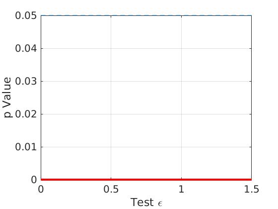
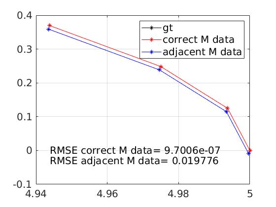
For a fixed sensor setup $\mathbf{Q_{1}}$ , we now report on the numerical results. We first show the simulation results when no entropy term exists ( $s_{k}=1,\forall k$ in Theorem 4 of [9]. We use $s$ to denote $s_{k},\forall k$ below). In Figure 4, from the left figure, the $p$ -value is always equal to 0, which means that the null hypothesis should always be rejected for all test $\varepsilon$ . Thus, the two sets of sensor data are distinguishable when $s=1$ . On the other hand, the estimate RMSE error using the correct sensor data generated from $\mathbf{Q_{1}}$ ( $E_{\textup{correct}}$ ) is almost zero and much smaller than $E_{\textup{adjacent}}$ . This error ( $E_{\textup{adjacent}}$ ) employs sensor data that are in fact generated from adjacent sensor positions to $\mathbf{Q_{1}}$ .

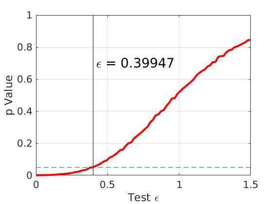
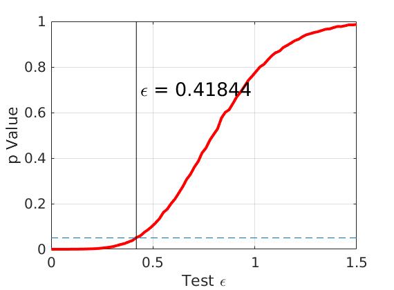
Then, we set $s=0.8$ and the simulation results are shown in Figure 5 (left figure). We obtain the critical value $\varepsilon_{c}=0.39947$ , where the $p$ -value is larger than 0.05. This means that the null hypothesis is not rejected and we accept that differential privacy holds for $\varepsilon\geq 0.39947$ , and $d=10$ and these two sensor data sets. The corresponding estimate errors are found to be $E_{\textup{{correct}}}=0.0040408$ and $E_{\textup{\text{adjacent}}}=0.026032$ for the estimates using the sensor data generated from $\mathbf{Q_{1}}$ and adjacent sensor positions, respectively. Recall that $s=0.8$ implies a relatively low noise injection level.

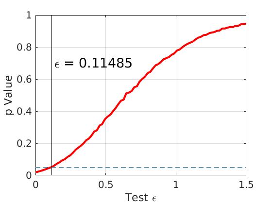
Decreasing $s$ to 0.7, leads to a larger entropy term in the $W_{2}$ -MHE: as shown in Figure 5 (right figure), the critical $\varepsilon_{c}$ becomes smaller ( $\varepsilon_{c}=0.11485$ ), confirming that a higher level of $(\varepsilon$ , $d$ -adj $)$ differential privacy is achieved. There is also a decrease in accuracy, which can be seen from $E_{\text{correct}}=0.00599996$ .

Therefore, the tests reflect the expected trade-off between differential privacy and accuracy. In order to choose between two given estimation methods, a designer can either (i) first set a bound on what is the tolerable estimation error, then compare two methods based on the differential privacy level they guarantee based on the given test, or (ii) given a desired level of differential privacy, choose the estimation method that results into the smallest estimation error.

Regarding the approximation term $\lambda$ , we can compute their values as discussed in Section IV-B. For each event $E_{i}$ , $\mathbb{P}(E_{i})$ can be approximated as $c_{1}/n$ , so $\eta$ is obtained via $\max(\mathbb{P}(E_{i}))$ ; $\beta=0.05$ is fixed and $\varepsilon_{c}$ values are known from tests. Therefore, when $s=0.8$ , we get $\eta=0.013$ and $\lambda=0.0888$ ; $s=0.7$ , we get $\eta=0.010$ and $\lambda=0.0724$ .

Input Perturbation.

The work [8] proposes two approaches to obtain differentially-private estimators. The first one randomizes the output of regular estimator ( $W_{2}$ -MHE belongs to this class). The second one perturbs the sensor data, which is then filtered through the original estimator. An advantage of this approach is that users do not need to rely on a trusted server to maintain their privacy since they can themselves release noisy signals. The question is which of the two approaches can lead to a better estimation result for the same level of differential privacy.

We can now compare these approaches numerically for the $W_{2}$ -MHE estimator method. By selecting $s=1$ and adding a Gaussian noise directly to both sets of adjacent sensor data, we re-run our test to find the trade-off between accuracy and privacy. The Gaussian noise has zero mean and the covariance matrix $Q=(1-\bar{s})(I+\frac{R+R^{\prime}}{2})$ , where, $I$ is the identity matrix and $R$ is a matrix of random numbers inl $(0,1)$ . A value $\bar{s}\in[0,1]$ quantifies how much the sensor data is perturbed. In simulation, we change the value of $\bar{s}$ and compare the results.

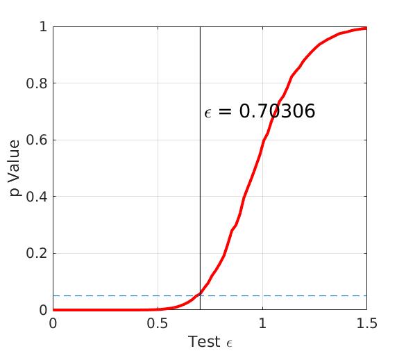
We first set $\bar{s}=0.944$ in $Q$ , see Figure 6 (left figure). The $\varepsilon_{c}$ and estimate error are found to be $\varepsilon_{c}=0.70306,E_{\text{correct}}=0.0010771$ and $\lambda=0.1550$ . Then, we decrease $\bar{s}=0.894$ , see Figure 6 (right figure). We obtain $\varepsilon_{c}=0.41844$ , $E_{\text{correct}}=0.0013998$ and $\lambda=0.1351$ . They also show that the higher level of differential privacy is achieved at the loss of accuracy. For the four cases, $\lambda$ values are not significant, indicating the approximation method is meaningful.

From ( $s=0.8$ , $\varepsilon_{c}=0.39947$ , $E_{\text{correct}}=0.0040408$ ) and ( $\bar{s}=0.894$ , $\varepsilon_{c}=0.41844$ , $E_{\text{correct}}=0.0013998$ ), we find that although the level of differential privacy is close to each other, the estimate error of $\bar{s}=0.894$ is only $1/3$ of that of $s=0.8$ . Thus, the second mechanism (adding noise directly at the mechanism input) seems to indicate that it can lead to better accuracy while maintaining the same $(\varepsilon$ , $d$ -adj $)$ differential privacy guarantee for this set of sensors.

We further compare the performances of the two mechanisms on other sensor setups (e.g. uniformly located on the circle), see Table I.

Sensor Setup	$W_{2}$ MHE	Input Perturbation	Better choice
$\mathbf{Q_{2}}$	$\varepsilon_{c}=0.53229$	$\varepsilon_{c}=0.72204$	$W_{2}$ -MHE
	$\lambda=0.1011$	$\lambda$ =0.2106
	$E_{\text{correct}}=0.0049874$	$E_{\text{correct}}=0.0049674$
$\mathbf{Q_{3}}$	$\varepsilon_{c}=0.98768$	$\varepsilon_{c}=2.3423$	$W_{2}$ -MHE
	$\lambda=0.1037$	$\lambda=0.8408$
	$E_{\text{correct}}=0.0030866$	$E_{\text{correct}}=0.0037826$

TABLE I: Comparisons of two mechanisms

From the table, we see that performance depend on the specific sensor setups. In 2 out of 3 sensor setups, perturbing the filter output seems the better option. However, more simulation results are needed to reach a reliable conclusion. Besides, we see that the approximation method works only when differential privacy holds ( $\varepsilon_{c}$ is relatively small).

Differentially private EKF [8].

The framework can also be applied to other differentially private estimators. For comparison, we evaluate the performance of an extended Kalman filter applied to the same examples. Compared EKF, random noise $\frac{1-\hat{s}}{\hat{s}}w$ ( $w$ is uniformly distributed over $[0,1]$ ) is added to the filter output at the update step, which makes the estimator differentially private. The initial guess $\mu_{0}$ is the same for the EKF and for the $W_{2}$ -MHE.

Table II illustrates the EKF test results. Compared with those of $W_{2}$ -MHE, the performance of the EKF remains to be worse than that of $W_{2}$ -MHE with respect to both privacy level and RMSE (for all sensor setups). This is consistent with the fact that $W_{2}$ -MHE performs better than the EKF for multi-modal distributions.

Sensor Setup	$\varepsilon_{c}$	$E_{\text{correct}}$	Better choice
$\mathbf{Q_{1}}$	$\quad 0.46223\quad$	$\quad 0.0066205\quad$	$W_{2}$ -MHE
$\mathbf{Q_{2}}$	$\quad 1.9239\quad$	$\quad 0.0064686\quad$	$W_{2}$ -MHE
$\mathbf{Q_{3}}$	$\quad 2.3085\quad$	$\quad 0.0062608\quad$	$W_{2}$ -MHE

TABLE II: Diff-private EKF test results

Correctness of sufficient condition for $W_{2}$ -MHE.

Theorem 4 of [9] provides with a theoretical formula to calculate $s$ that guarantees $(\varepsilon$ , $d$ -adj $)$ differential privacy. Since this condition is derived using several assumptions and upper bounds, the answer is in general expected to be conservative.

In order to make comparisons, we choose the sensor setup $\mathbf{Q_{2}}$ and take $s=0.8$ for simulation. The value of other parameters are: $T=7\text{ (for less computation)},c_{f}=1.0777,c_{h}=100,l=1293.2(N=5),\operatorname{diam}(\mathcal{K}_{0})=0.1,{\color[rgb]{0,0,0}\definecolor[named]{pgfstrokecolor}{rgb}{0,0,0}\pgfsys@color@gray@stroke{0}\pgfsys@color@gray@fill{0}d}=10$ . Plug these values into the theorem, we can obtain $\varepsilon\geq 6474.3$ . In simulation, the critical $\varepsilon_{c}$ = 0.89281. Upon inspection, it is clear that the theoretical answer is much more conservative than the approximated one, which indicates that if $\varepsilon\geq 0.89281$ , differential privacy is satisfied with high confidence wrt the given space partition. While this is a necessary condition for privacy, we run a few more simulations to test how this changes for finer space partitions.

1.

$r=3$ (9 regions per time step), $\varepsilon_{c}=0.98162$
2.

$r=4$ (16 regions per time step), $\varepsilon_{c}=1.9939$
3.

$r\geq 5$ , much more computation are required (numebr of events increases exponentially)

As observed, a finer space partition leads an increase of $\varepsilon_{c}$ . But the theoretical bound is still far from the observed values.

VI CONCLUSION

This work presents a numerical test framework to evaluate the differential privacy of continuous-range mechanisms such as state estimators. This includes a precise quantification of its performance guarantees. Then, we apply the numerical method on differentially-private versions of the $W_{2}$ -MHE filter, and compare it with other competing approaches. Future work will be devoted to obtain more efficient algorithms that; e.g., refine the considered partition adaptively.

References

[1] A. Narayanan and V. Shmatikov, “How to break anonymity of the netflix prize dataset,” preprint arxiv:cs/0610105, 2006.
[2] B. Hoh, T. Iwuchukwu, Q. Jacobson, D. Work, A. M. Bayen, R. Herring, J. Herrera, M. Gruteser, M. Annavaram, and J. Ban, “Enhancing privacy and accuracy in probe vehicle-based traffic monitoring via virtual trip lines,” IEEE Transactions on Mobile Computing, 2012.
[3] C. Dwork, M. Frank, N. Kobbi, and S. Adam, “Calibrating noise to sensitivity in private data analysis,” in Theory of Cryptography, 2006.
[4] J. Cortes, G. E. Dullerud, S. Han, J. L. Ny, S. Mitra, and G. J. Pappas, “Differential privacy in control and network systems,” in IEEE Int. Conf. on Decision and Control, 2016, pp. 4252–4272.
[5] Y. Wang, Z. Huang, S. Mitra, and G. E. Dullerud, “Entropy-minimizing mechanism for differential privacy of discrete-time linear feedback systems,” in IEEE Int. Conf. on Decision and Control, 2014.
[6] E. Nozari, P. Tallapragada, and J. Cortes, “Differentially private distributed convex optimization via functional perturbation,” IEEE Transactions on Control of Network Systems, 2019.
[7] J. L. Ny, “Privacy-preserving filtering for event streams,” preprint arXiv: 1407.5553, 2014.
[8] J. L. Ny and G. J. Pappas, “Differentially private filtering,” IEEE Transactions on Automatic Control, pp. 341–354, 2014.
[9] V. Krishnan and S. Martínez, “A probabilistic framework for moving-horizon estimation: Stability and privacy guarantees,” IEEE Transactions on Automatic Control, pp. 1–1, 06 2020.
[10] Y. Chen and A. Machanavajjhala, “On the privacy properties of variants on the sparse vector technique,” 2015.
[11] M. Lyu, D. Su, and N. Li, “Understanding the sparse vector technique for differential privacy,” 2016.
[12] Z. Y. Ding, Y. X. Wang, G. H. Wang, D. F. Zhang, and D. Kifer, “Detecting violations of differential privacy,” Proc.s of the 2018 ACM SIGSAC Conference on Computer and Communications Security.
[13] A. Devonport and M. Arcak, “Estimating reachable sets with scenario optimization,” in Annual Learning for Dynamics & Control Conference, 2020.
[14] R. A. Fisher, The design of experiments, 1935.

	$\displaystyle\mathbb{P}(\mathcal{M}(\mathrm{y}_{0:T}^{1})\in E)$
	$\displaystyle=\mathbb{P}(\mathcal{M}(\mathrm{y}_{0:T}^{1})\in E\|R)\mathbb{P}(R)+\mathbb{P}(\mathcal{M}(\mathrm{y}_{0:T}^{1})\in E\|\overline{R})\mathbb{P}(\overline{R})$
	$\displaystyle\leq e^{\varepsilon}\mathbb{P}(\mathcal{M}(\mathrm{y}_{0:T}^{2})\in E\|R)\mathbb{P}(R)+\theta\mathbb{P}(\mathcal{M}(\mathrm{y}_{0:T}^{1})\in E\|\overline{R})\leq$
	$\displaystyle e^{\varepsilon}[\mathbb{P}(\mathcal{M}(\mathrm{y}_{0:T}^{2})\in E\|R)\mathbb{P}(R)+\mathbb{P}(\mathcal{M}(\mathrm{y}_{0:T}^{2})\in E\|\overline{R})\mathbb{P}(\overline{R})]+\theta$
	$\displaystyle=e^{\varepsilon}\mathbb{P}(\mathcal{M}(\mathrm{y}_{0:T}^{2})\in E)+\theta,$

A Numerical Verification Framework for Differential Privacy in Estimation

Abstract

I INTRODUCTION

II Problem Formulation

Definition 1

III Approximate (ε(\varepsilon,dd-adj)) Differential Privacy

Definition 2

Lemma 1

Proof:

Definition 3 (Differential privacy wrt a space partition)

Lemma 2

Proof:

Lemma 3

Proof:

IV Differential Privacy Test Framework

IV-A Overview of the differential-privacy test framework

IV-A1 EventListGenerator module.

Lemma 4

Proof:

IV-A2 WorstEventSelector module.

IV-A3 HypothesisTest module.

Lemma 5 ([12].)

IV-B Theoretical Guarantee

Theorem 1

Proof:

V EXPERIMENTS

System Example.

dd-adjacent sensor data.

Input Perturbation.

Differentially private EKF [8].

Correctness of sufficient condition for W2W_{2}-MHE.

VI CONCLUSION

References

III Approximate $(\varepsilon$ , $d$ -adj $)$ Differential Privacy

$d$ -adjacent sensor data.

Correctness of sufficient condition for $W_{2}$ -MHE.