A one-dimensional mixing model for the impact of ablative Rayleigh-Taylor instability on compression dynamics

Laboratory fusion ignition [1, 2] has been successfully achieved at the National Ignition Facility (NIF) through the central ignition scheme[3, 4]. In this scheme, a hot spot is generated in the center of the fuel shell, a spark of nuclear fusion is initiated, and a burning wave propagates through the shell when the ignition threshold is surpassed. Both the formation of the hot spot and the propagation of the burning wave are closely related to the dynamics of compression[5, 6, 7]. Extensive experimental studies have observed compression degradation[8, 9, 10, 11, 12, 13, 14, 15], as quantified by key parameters such as adiabat, areal density, and inflight shell thickness. To understand this degradation, researchers have investigated the underlying physical mechanisms in various phases of implosion.

The compression dynamics is significantly influenced by hydrodynamic instabilities across various scales. Low-mode drive asymmetries [16, 17], originating from hohlraum geometry and cross-beam energy transfer (CBET) [18, 19], have been identified as primary contributors to reduced fuel compression at stagnation. High-mode non-uniformities at fuel-ablator interface [20, 21] enhance fuel entropy through mixing, thereby reducing compression in the acceleration phase, a process exacerbated by preheating effects[22, 23, 24, 25]. Moreover, high-mode ablative Rayleigh-Taylor instability (ARTI), seeded by target defects [26, 27] and laser imprint [28, 29], fosters the mixing of hot and cold plasmas, thus decreasing compression by affecting laser ablation prior to the onset of these instabilities.

Because of the vast parameter space associated with high-dimensional simulations [30, 31], previous studies have employed one-dimensional (1D) simulations that utilize various adjustable multipliers to investigate the effects of mixing in various phases. For example, the fall-line mix model [32] modifies the fusion process by introducing an adjustable multiplier that calibrates the width of fully atomized mixing region during the deceleration phase. Moreover, at CH-DT interface, plasma flows within the mixing region, as refined by the buoyancy-drag (BD) model[33], have been modified using either a surface-to-volume (AOV) multiplier [34, 35] or through 1D Reynolds-averaged Navier-Stokes equations[36, 37] with coefficients tailored for turbulent phases. However, these existing models are not readily applicable to ARTI due to their insufficient treatment of laser ablation effects and initial perturbations.

In this paper, we develop a 1D mixing model that incorporates the effects of laser ablation and initial perturbations to study the impact of ARTI on compression dynamics. The length of the mixing region is calculated using a BD model [38] with a time-varying drag coefficient. The mixing effect on laser ablation is characterized through a perturbed heat source, parameterized by turbulent kinetic energy and initial perturbation level via a free multiplier. The model is then integrated into a one-dimensional radiation hydrodynamics code and validated against two-dimensional planar simulations. Subsequent application to spherical implosion simulations reveals that the model can give reasonable predictions of implosion degradation due to mixing, such as lowered shell compression, reduced stagnation pressure, decreased areal density, and shortened time interval between the convergence of the main shock and stagnation. Notable, this interval may offer an estimate of mixing level in single-shot experiments.

The paper is organized as follows. We elaborate the 1D mixing model based on simulations in Section 2. We implement the model into the code MULTI-IFE [39] and validate it against FLASH [40] simulations in planar geometry in Section 3. We apply the model to implosion dynamics analysis in Section 4. Finally, we draw our conclusions in section 5.

In inertial confinement fusion (ICF), high-mode nonlinear ARTI induces significant mixing between hot and cold plasmas, profoundly affecting laser ablation process. This phenomenon is characterized by an increased characteristic scale length of the ablation front, as evidenced by FLASH [40] simulations. To investigate this effect in the mixing region refined by the BD model, we develop a 1D mixing model that uses a perturbed heat source to calculate the mixing effects on laser ablation.

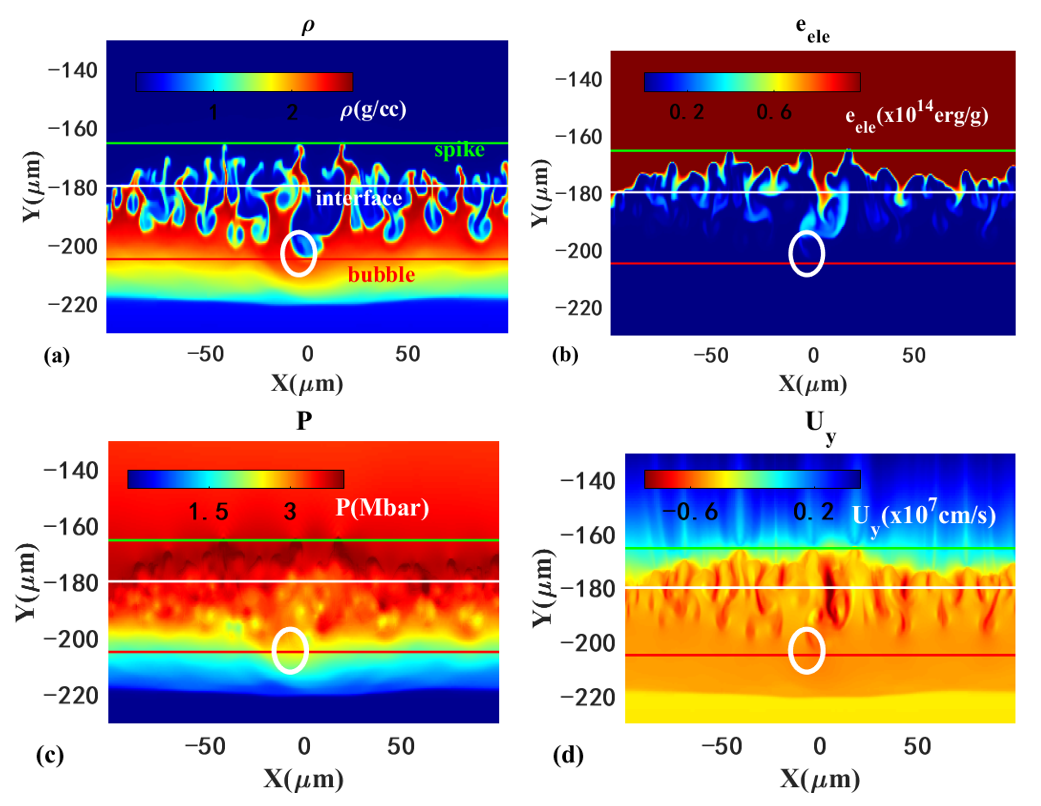
We begin by analyzing the influence of ARTI on flow fields. As dipicted in figure 1, the mixing region is defined as the zone between the bubble front and the spike front. Large bubbles, indicated by white ellipses, demonstrate a notable decrease in density in figure 1(a), and an obvious increase in the specific internal energy of electrons in figure 1(b), pressure in figure 1(c) and velocity in the Y direction in figure 1(d) compared to ideal uniform distributions in the X direction. These approximate uniform distributions in the X direction motivate our development of a 1D mixing model based on spatially averaged hydrodynamic equations. These equations encompass the mass conservation equation, the momentum equation and the internal energy equation, which are expressed as follows:

	$\displaystyle\frac{\partial\rho}{\partial t}+\frac{\partial\rho{{U}_{j}}}{\partial{{x}_{j}}}=0,$		(1a)
	$\displaystyle\frac{\partial\rho{{U}_{i}}}{\partial t}+\frac{\partial\rho{{U}_{i}}{{U}_{j}}}{\partial{{x}_{j}}}=-\frac{\partial P}{\partial{{x}_{i}}},$		(1b)
	$\displaystyle\frac{\partial\rho e}{\partial t}+\frac{\partial\rho{U}_{j}e}{\partial{x}_{j}}=-P\frac{\partial{U}_{j}}{\partial{{x}_{j}}}-\frac{\partial q_{j}}{\partial{{x}_{j}}},$		(1c)

where $P$ represents pressure, $e$ denotes specific internal energy, and $\vec{q}=\vec{q}_{ele}+\vec{q}_{rad}$ is the total heat flux that has a radiation and electron conductivity component. The electron conductivity is given by ${q}_{ele,j}=-\kappa_{ele}\frac{\partial T_{ele}}{\partial{{x}_{j}}},$ where $\kappa_{ele}$ is the coefficient of electron conductivity, proportional to $T_{ele}^{5/2},$ and $T_{ele}$ represents the electron temperature.

The averaging process involves a spatial average ($\rho=\bar{\rho}+\rho^{\prime}$) and a mass-weighted average ($U=\overline{\overline{U}}+U^{\prime\prime}$). The relationship between these two averages is characterized by

$$\overline{\overline{U}}=\frac{\overline{\rho U}}{\bar{\rho}}=\overline{U}+\frac{\overline{\rho^{\prime}U^{\prime}}}{\bar{\rho}},\bar{\rho}=\int\limits_{0}^{L_{x}}{\rho dX}/\int\limits_{0}^{L_{x}}{dX},$$

where $\bar{\rho}$ and $\rho^{\prime}$ represent the mean and fluctuating density of the spatial average, while $\overline{\overline{U}}$ and $U^{\prime\prime}$ denote the mean and fluctuating velocity of the mass-weighted spatial average. Upon averaging, equation (1a) transforms into the form as one-dimensional mass conservation equation:

$$\frac{\partial\bar{\rho}}{\partial t}+\frac{\partial\bar{\rho}{{{\overline{\overline{U}}}}_{y}}}{\partial{y}}=0.$$

(1b)

Similarly, equation (1b) becomes

$$\frac{\partial\bar{\rho}{{{\overline{\overline{U}}}}_{y}}}{\partial t}+\frac{\partial\bar{\rho}{{{\overline{\overline{U}}}}_{y}}{{{\overline{\overline{U}}}}_{y}}}{\partial{y}}=-\frac{\partial\overline{P}}{\partial{y}}-\frac{\partial\overline{\rho{{U}_{y}}^{\prime\prime}{{U}_{y}}^{\prime\prime}}}{\partial{y}}.$$

(1c)

The right-hand side of equation (1c) consists of two components: the pressure gradient and the shear force associated with the velocity gradient. The shear force serves as the source of turbulent kinetic energy, defined as ${K}_{f}=\frac{1}{2}\frac{\overline{\rho U_{i}^{{}^{\prime\prime}}U_{i}^{{}^{\prime\prime}}}}{\overline{\rho}}$. During the implosion process, the inflight shell moves on the order of hundreds of micrometers, while the bubble’s movement is limited to few tens of micrometers to maintain shell integrity. Consequently, the perturbed velocity constitutes at most 10% of the implosion velocity, and ${K}_{f}$ accounts for less than 1% of the total kinetic energy $\overline{\overline{E}}_{k}$. This context allows us to neglect the influence of the shear force , which is further supported by the larger pressure gradient than the velocity gradient in the Y direction near the ablation front, as illustrated in figure 1(c) and (d).

Moreover, disregarding the correlations in $\vec{q}_{rad}$, the averaged internal energy equation can be expressed as follows:

$$\frac{\partial\bar{\rho}\bar{\bar{e}}}{\partial t}+\frac{\partial\bar{\rho}\overline{\overline{U}}_{y}\bar{\bar{e}}}{\partial y}=-\overline{P}\frac{\partial\overline{\overline{U}}_{y}}{\partial{y}}-\frac{\partial\bar{q}_{rad,y}}{\partial{y}}-\frac{\partial{\kappa_{ele}(\overline{\overline{T}}_{ele})\frac{\partial\overline{\overline{T}}_{ele}}{\partial{y}}}}{\partial{y}}+W,$$

(1d)

where $W$ is expressed as

$$W=-\frac{\partial\overline{\rho{U}_{y}^{{}^{\prime\prime}}e^{{}^{\prime\prime}}}}{\partial y}-\overline{P\frac{\partial{U}_{y}^{{}^{\prime\prime}}}{\partial{y}}}-(\frac{\partial{\bar{q}_{ele,y}}}{\partial{y}}-\frac{\partial{\kappa_{ele}(\overline{\overline{T}}_{ele})\frac{\partial\overline{\overline{T}}_{ele}}{\partial{y}}}}{\partial{y}}),$$

including correlations from diffusion, compression work and thermal conduction. The term in bracket with the highest degree of $T_{e}^{7/2}$ presents substantial challenges in developing accurate closure models. Therefore, recognizing that equation (1b) and (1c) share the same form as one-dimensional equations when neglecting the shear force, we develop a phenomenological mixing model to address $W$ in equation (1d).

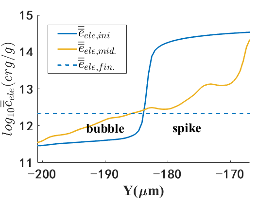
The spatial extent of the mixing model is determined based on the average characteristic of ${{e}_{ele}}$, as represented by the yellow line in figure 2. This average characteristic indicates that mixing enhances the characteristic scale length of the ablation front, leading to an evolution from the initial state ${{\bar{\bar{e}}}_{ele,ini.}}$ to the middle mixing state ${{\bar{\bar{e}}}_{ele,mid.}}.$ Notably, ${{\bar{\bar{e}}}_{ele,mid.}}$ at both the spike front and the bubble front closely resembles ${{\bar{\bar{e}}}_{ele,ini.}}$ , underscoring the mixing region as the primary area influenced by ARTI. Therefore, the mixing region is calculated using the BD model[38], expressed as follows:

$$\frac{d{{V}_{B}}}{dt}={{A}_{t}}g-D\frac{{{V}_{B}}\left|{{V}_{B}}\right|}{{{h}_{B}}},$$

(1e)

where $D(t),\,A_{t}(t)$ and $g(t)$ represent the time-varying drag coefficient, Atwood number and acceleration, respectively. The center of the mixing region is located at the ablation front, extending a length of $h_{B}$ above and below.

The computation of $W$ in equation (1d) is based on the relaxation of a perturbed heat source. We assume that the system evolves toward a final isothermal state, denoted as $\bar{\bar{e}}_{ele,fin.}(t,\Delta t).$ In the absence of ablative flux, characterized by $V_{a}=0$ and $K_{f}/\overline{\overline{E}}_{k}=1,$ the isothermal state can be achieved over a relaxation time $\Delta t$, where $V_{a}$ represents the averaged ablative velocity. The maximum perturbed heat source is defined as

$$\Delta{\bar{\bar{e}}_{ele}(t,\Delta t,y)}={\bar{\bar{e}}_{ele,fin.}(t,\Delta t)}-{\bar{\bar{e}}_{ele,ini.}(t,y)},$$

which exhibits positive values near bubbles and negative values near spikes, as illustrated in figure 2. Consequently, the perturbed heat source in equation (1fa) is formulated as $\aleph(t,y)\Delta{{\bar{\bar{e}}}_{ele}(t,\Delta t,y)}$ and is utilized to close $W$:

	$\displaystyle W=\frac{\partial Q_{per.}(t,y)}{\partial t}=\frac{\aleph(t,y)\Delta{{\bar{\bar{e}}}_{ele}(t,\Delta t,y)}}{\lambda/V_{a,loc}(t)},$		(1fa)
	$\displaystyle\aleph(t,y)=\sqrt{K_{f}(t,y)/\overline{\overline{E}}_{k}(t,y)}\times{\xi(t)}^{-1/2(-1+sign(\Delta{{{\bar{\bar{e}}}}_{ele}(t,y)}))},$		(1fb)
	$\displaystyle{{K}_{f}(t,y)}={\frac{1}{2}{f}_{mix}}V_{B}(t)^{2}(1-{{y}^{2}}/h_{B}^{2}),$		(1fc)
	$\displaystyle{\int\limits_{V\in mix\,region}W\times\rho dV}=0.$		(1fd)

Here, the relaxation time of the heat source is defined as $\lambda/V_{a,loc}(t),$ where $\lambda$ is the dominant perturbation wavelength at the onset of acceleration and the local ablative velocity $V_{a,loc}(t)$ approximates the ablative velocity from 1D simulations. The amplitude of the heat source is associated with the mixing level, represented by $\aleph(t,y)$ in equation (1fb), where the $sign$ function is defined as:

$$sign(x<0)=-1,sign(x>0)=1,sign(x=0)=0.$$

Additionally, a specific spatial distribution of ${{K}_{f}}$ is assumed, similar to that used in the RANS model [36], as expressed in equation (1fc). $\xi$(t) in equation (1fd) ensures that the integral of the perturbed heat source within the mixing region equals zero.

In equation (1fb), $\aleph(t,y)$ is proportional to the percentage of specific turbulent kinetic energy, expressed as $\sqrt{K_{f}(t,y)/\overline{\overline{E}}_{k}(t,y)},$ whose function form may vary. Although $K_{f}(t,y)$ does not evolve according to equation (1c) in the absence of the shear force, its maximum value can be defined as $\frac{1}{2}f_{mix}V_{B}^{2}(t)$, occurring near the interface between bubbles and spikes, specially at the ablation front, as illustrated in figure 1(d). Here, ${{f}_{mix}}$ is an adjustable multiplier that characterizes the initial perturbation level at the onset of acceleration. For example, if only a local defect is present at the ablation front, ${{f}_{mix}}$ approaches the lower limit of zero, whereas a fully perturbed ablation front results in ${{f}_{mix}}$ approaching the upper limit of one. We also recognize that the mixing level can be manipulated in two distinct ways: by changing the time evolution of $h_{B}$ and by adjusting ${{f}_{mix}}$. The effects of these two ways are obviously different, suggesting the complexity of mixing dynamics at the ablation front.

Eventually, to address $W$ in equation (1d), the phenomenological mixing model explicitly calculates the relaxation of the perturbed heat source, as expressed in equation (1fg):

$${\bar{\bar{e}}_{ele,mid.}(t,dt,y)-\bar{\bar{e}}_{ele,ini.}(t,y)}=W\times dt,$$

(1fg)

during the lookup process of equation of state (EOS), where $dt$ is the time step. Furthermore, within the mixing region, thermal relaxation promotes the equilibration of temperatures between electrons and ions, resulting in a corresponding 1D mixing model for the mass-weighted spatially averaged specific internal energy of ions. The integration of the model will be detailed in the following section.

In MULTI-IFE, the hydrodynamic evolution is consistent with equation (1b-1d), while incorporating the implementation of equation (1e), and equation (1fg) is explicitly calculated to describe the correlations in (1d) prior to the EOS table lookup[39]. When the time evolution of the mixed region is confirmed, we determine ${{f}_{mix}}$ via ensuring the calculation results consistent with that of 2D simulations.

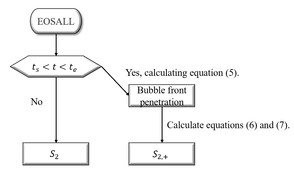
The implementation process begins by defining several global input parameters, such as the initial perturbations, the onset time ${{t}_{s}}$ when perturbations enter the nonlinear phase[41], and the end time ${{t}_{e}}$ marking the end of the acceleration phase. These parameters are essential for calculating ${{V}_{B}}$ and ${{h}_{B}}$ using equation (1e). As illustrated in figure 3, from $t={{t}_{s}}$ to $t={{t}_{e}}$, $\bar{\bar{e}}$ is updated according to equation (6) and (1fg), leading to corresponding updates in temperature, pressure and other relevant parameters. By inferring ${{f}_{mix}}$, these updated parameters enhance the consistency of the mixing model with the averaged results obtained from two-dimensional simulations.

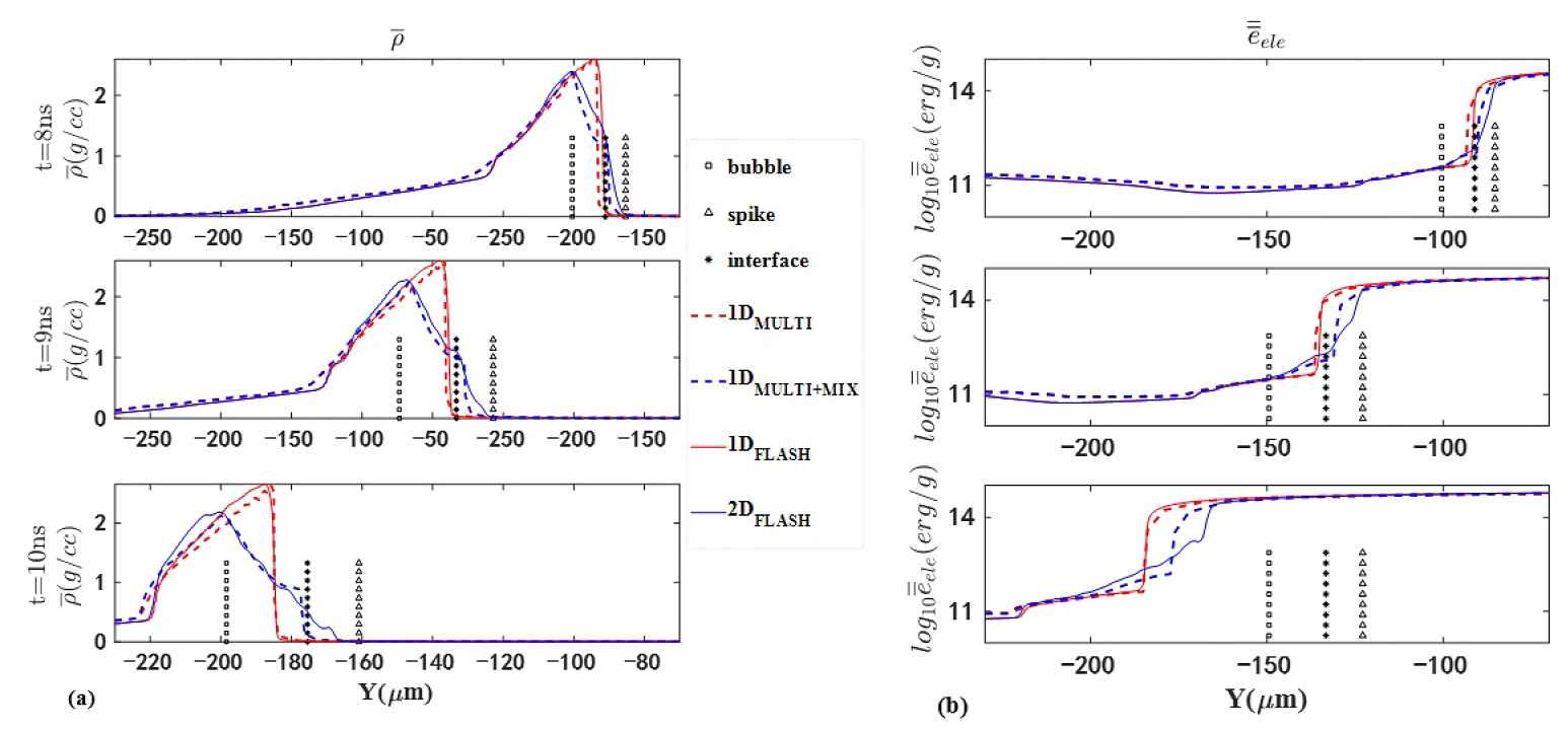
The results of the mixing model applied to laser-ablated planar targets are presented in figure 4(a) and (b). In these figures, solid lines represent FLASH simulations, while dashed lines correspond to MULTI-IFE simulations. Blue lines denote simulations with initial velocity perturbations, whereas red lines indicate simulations without perturbations. The overlapping red lines imply that the time evolution of $\bar{\rho}$ and $\bar{\bar{e}}_{{ele}}$ is similar in both simulations, despite differences in computational cells. In the presence of perturbations, the 2D simulation observes an increase in ${{\bar{\bar{e}}}_{ele}}$ and a decrease in $\bar{\rho}$ near the bubble front, while an opposite trend is observed near the spike front. Notably, mixing causes the maximum specific internal energy gradient of electrons to shift outward into the coronal region. Our 1D mixing model effectively captures the time evolution of these characteristics with ${{f}_{mix}}=0.03,$ however, a notable deviation is observed near the spike front, which is anticipated due to the increased values of $\Delta\bar{\bar{e}}_{ele}$ in this region, as illustrated in figure 2.

We further quantify the compression of the implosion shell, defined as the region between the internal and external points where the density equals $1/e$ of the maximum density. At $t=10$ ns, the compression of the inflight shell, represented by the average density in planar geometry and mass-weighted adiabat, decreases by approximately $50\%$ when mixing is considered. Specifically, the average density and mass-weighted adiabat of the implosion shell from 2D FLASH simulations are 1.58 g/cc and 1.77, while the values calculated by 1D MULTI-IFE are 1.49 g/cc and 1.62. The relative errors for average density (5.7%) and mass-weighted adiabat (8.5%) both remain below $10\%$ .

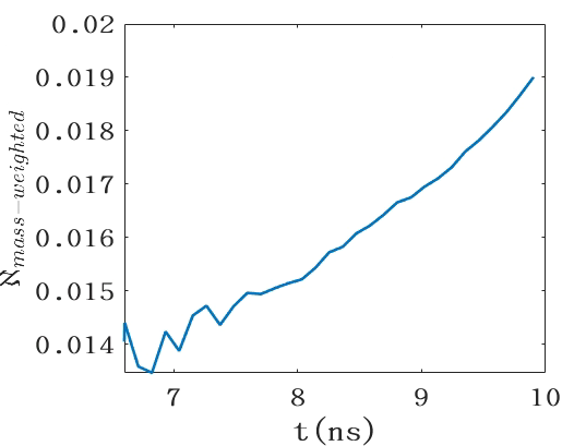
Furthermore, We define the mass-weighted mixing level as

$$\aleph_{mass-weighted}(t)=\frac{\int\limits_{V\in mix\,region}{\left(\aleph(t,y)\rho dV\right)}}{\int\limits_{V\in mix\,region}{\left(\rho dV\right)}},$$

with its time evolution illustrated in figure 5. During the development of instabilities, the mixing level, as indicted using $K_{f}$, increases over time. Ultimately, the relationship between the evolving instabilities and the rising mixing level enhances our comprehension of mixing.

Implosion experiments have measured several typical phenomena, including the reduced compression of the inflight shell, lowered stagnation pressure, decreased areal density of the hot spot and early onset of bang time [42, 43]. To investigate the relationship between these phenomena and mixing, we implement the model in spherical geometry. In this context, $\bar{\bar{e}}_{ele,fin.}$ is calculated using the formula:

$$\bar{\bar{e}}_{ele,fin.}=\int\limits_{R}4\pi{R}^{2}\bar{\rho}\bar{\bar{e}}_{ele,ini.}dR/\int\limits_{R}4\pi{R}^{2}\bar{\rho}dR.$$

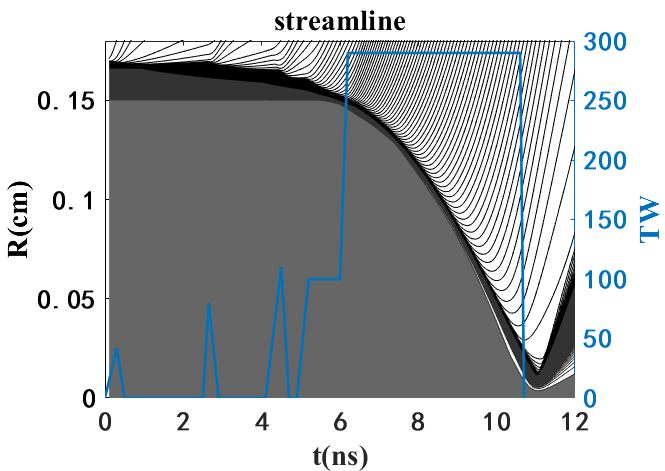
Figure 6 presents the pulse shape and streamline diagram for a 1.5-MJ triple-picket design [44]without the mixing model. The typical target scheme is reflected through grayscale: the outer plastic has a density of 1 g/cc, the middle DT ice has a density of 0.25 g/cc, and the inner DT gas has a density of 6 mg/cc. The inflight shell begins to accelerate at $t=5.5$ ns, continuing until the main shock reflects from the center to the interior of the inflight shell at $t=10.5$ ns, marking the onset of the deceleration phase. At approximately 11 ns, the hot spot stagnates, characterized by its minimum volume.

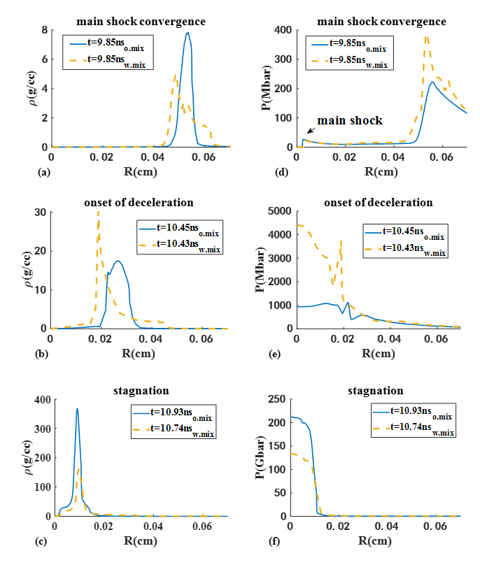
During the acceleration phase from 5.5 ns to 10.5 ns, we employ the mixing model at the ablation front with $f_{mix}=0.03$ , as calibrated in Section 3. The quality of the hot spot at three characteristic moments are detailed in figure 7. The outer radius of the hot spot is denoted by the maximum density gradient. In figure 7(a), the mixing model predicts a decreased inner radius^[11] accompanied by an increased thickness of the inflight shell, indicative of decreased compression. Notably, the convergent time of the main shock, shown in figure 7(d), remains unaffected by mixing, because it occurs with only minor perturbations at the onset of acceleration. The combination of reduced hot spot radius and spherical convergence geometry results in enhanced density and pressure within the hot spot at the onset of deceleration, as demonstrated in figures 7(b) and (e). Differently, the expanded radius caused by mixing effects leads to decreased density and pressure within the hot spot at stagnation, as shown in figures 7(c) and (f). Moreover, Changes in implosion dynamics caused by mixing contribute to an earlier onset of the deceleration phase and the stagnation. These phenomena suggest that mixing may lead to an earlier bang time^{[42, 43]}.

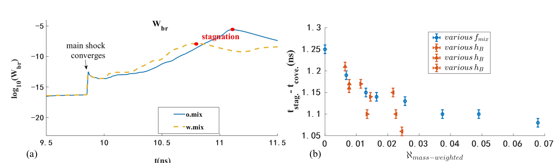
The self-emissivity signal of the hot spot can indicate the moment of stagnation and the quality of the hot spot, making it an indicator of the mixing level. We present the total bremsstrahlung energy of the hot spot within a radius of 10 um, i.e.,

$${{W}_{br}}\sim\int{{{\rho}^{2}}{{T}_{e}}^{1/2}dV}.$$

As seen in figure 8 (a), the peak of X-ray self-emission with mixing is much lower than that without mixing. Furthermore, the interval between the convergence of the main shock and stagnation is reduced. We then conducted simulations to investigate the relationship between the interval and the mass-weighted mixing level at the end of acceleration, denoted as $\aleph_{mass\,weighted}.$ As illustrated in figure 8 (b), when $\aleph_{mass\,weighted}$ is varied using two different methods, both approaches reveal that the interval decreases as the mixing level increases, albeit at different extent. This decreasing trend may offer an estimate of mixing level in single-shot experiments.

To investigate the influence of ARTI on compression dynamics within a reduced parameter space, we present a one-dimensional mixing model that incorporates the effect of laser ablation and initial perturbations. The length of the mixing region is determined with a BD model. The mixing effect on laser ablation is mainly described with an additional heat source which depends on turbulent kinetic energy and initial perturbation level through a free multiplier. Following the successful implementation of the model, we calibrate the adjustable multiplier against two-dimensional planar simulations. Furthermore, the application of our model to spherical implosion simulations reveals that the model can give reasonable predictions of implosion degradation due to mixing, such as lowered shell compression, reduced stagnation pressure, and decreased areal density, etc. It is found that the time interval between the convergence of the main shock and stagnation may offer an estimate of mixing level in single-shot experiments. Overall, our model could serve as a valuable tool for evaluating the impact of ARTI on implosion dynamics, particularly for future schemes aimed at enhancing compression, such as the SQ-n design.[45, 46].

This work is supported by the supported by the National Key R and D Projects (Grant No. 2023YFA1608400), Strategic Priority Research Program of the Chinese Academy of Sciences (Grant No. XDA25010200), and Nature Science Foundation of China (Grant No. 12375242).

All data that support the findings of this study are included within the article (and any supplementary files).

References

- [1] Abu-Shawareb H, Acree R, Adams P, Adams J, Addis B, Aden R, Adrian P, Afeyan B, Aggleton M, Aghaian L et al. 2022 Physical Review Letters 129 075001
- [2] Abu-Shawareb H, Acree R, Adams P, Adams J, Addis B, Aden R, Adrian P, Afeyan B, Aggleton M, Aghaian L et al. 2024 Physical Review Letters 132 065102
- [3] Lindl J 1995 Physics of Plasmas 2 3933–4024
- [4] Hurricane O, Patel P, Betti R, Froula D, Regan S, Slutz S, Gomez M and Sweeney M 2023 Reviews of Modern Physics 95 025005
- [5] Nuckolls J, Wood L, Thiessen A and Zimmerman G 1972 Nature 239 139–142
- [6] Theobald W, Solodov A, Stoeckl C, Anderson K, Beg F, Epstein R, Fiksel G, Giraldez E, Glebov V Y, Habara H et al. 2014 Nature Communications 5 5785
- [7] Tommasini R, Landen O, Berzak Hopkins L, Hatchett S, Kalantar D, Hsing W, Alessi D, Ayers S, Bhandarkar S, Bowers M et al. 2020 Physical Review Letters 125 155003
- [8] Robey H, MacGowan B, Landen O, LaFortune K, Widmayer C, Celliers P, Moody J, Ross J, Ralph J, LePape S et al. 2013 Physics of Plasmas 20 052707
- [9] Thomas C, Campbell E, Baker K, Casey D, Hohenberger M, Kritcher A, Spears B, Khan S, Nora R, Woods D et al. 2020 Physics of Plasmas 27 112705
- [10] Yang W, Duan X, Li Y, Zhang Y, Jing L, Guan Z, Zhang C, Liu H, Zhang H, Dong Y et al. 2024 Nuclear Fusion 65 016032
- [11] Michel D, Hu S, Davis A, Glebov V Y, Goncharov V, Igumenshchev I, Radha P, Stoeckl C and Froula D 2017 Physical Review E 95 051202
- [12] Johnson M G, Frenje J, Casey D, Li C, Séguin F, Petrasso R, Ashabranner R, Bionta R, Bleuel D, Bond E et al. 2012 Review of Scientific Instruments 83 10D308
- [13] Frenje J A, Bionta R, Bond E, Caggiano J, Casey D, Cerjan C, Edwards J, Eckart M, Fittinghoff D, Friedrich S et al. 2013 Nuclear Fusion 53 043014
- [14] Landen O, Casey D, DiNicola J, Doeppner T, Hartouni E, Hinkel D, Hopkins L B, Hohenberger M, Kritcher A, LePape S et al. 2020 High Energy Density Physics 36 100755
- [15] Meaney K, Kim Y, Geppert-Kleinrath H, Herrmann H, Hopkins L B and Hoffman N 2020 Physical Review E 101 023208
- [16] Scott R, Clark D, Bradley D, Callahan D, Edwards M, Haan S, Jones O, Spears B, Marinak M, Town R et al. 2013 Physical Review Letters 110 075001
- [17] Rinderknecht H G, Casey D, Hatarik R, Bionta R, MacGowan B, Patel P, Landen O, Hartouni E and Hurricane O 2020 Physical Review Letters 124 145002
- [18] Kritcher A, Ralph J, Hinkel D, Döppner T, Millot M, Mariscal D, Benedetti R, Strozzi D, Chapman T, Goyon C et al. 2018 Physical Review E 98 053206
- [19] Edgell D, Radha P, Katz J, Shvydky A, Turnbull D and Froula D 2021 Physical Review Letters 127 075001
- [20] Cheng B, Kwan T J, Wang Y M, Yi S, Batha S H and Wysocki F J 2016 Physics of Plasmas 23 120702
- [21] Amendt P 2021 Physics of Plasmas 28 072701
- [22] Li J, Yan R, Zhao B, Zheng J, Zhang H and Lu X 2022 Matter and Radiation at Extremes 7 055902
- [23] Li J, Yan R, Zhao B, Wu J, Wang L and Zou S 2024 Physics of Plasmas 31 012703
- [24] Jones O, Suter L, Scott H, Barrios M, Farmer W, Hansen S, Liedahl D, Mauche C, Moore A, Rosen M et al. 2017 Physics of Plasmas 24 056312
- [25] Robey H, Boehly T, Celliers P, Eggert J, Hicks D, Smith R, Collins R, Bowers M, Krauter K, Datte P et al. 2012 Physics of Plasmas 19 042706
- [26] Pak A 2023 Overview of principal degradations arising from capsule target perturbations in inertial confinement fusion implosions Tech. rep. Lawrence Livermore National Laboratory (LLNL), Livermore, CA (United States)
- [27] Divol L, Pak A, Bachmann B, Baker K, Baxamusa S, Biener J, Bionta R, Braun T, Casey D, Choate C et al. 2024 Physics of Plasmas 31 102703
- [28] Goncharov V, Gotchev O, Vianello E, Boehly T, Knauer J, McKenty P, Radha P, Regan S, Sangster T, Skupsky S et al. 2006 Physics of Plasmas 13 012702
- [29] Liu D, Tao T, Li J, Jia Q and Zheng J 2022 Physics of Plasmas 29 072707
- [30] Clark D, Weber C, Milovich J, Salmonson J, Kritcher A, Haan S, Hammel B, Hinkel D, Hurricane O, Jones O et al. 2016 Physics of Plasmas 23 056302
- [31] Clark D, Weber C, Milovich J, Pak A, Casey D, Hammel B, Ho D, Jones O, Koning J, Kritcher A et al. 2019 Physics of Plasmas 26 050601
- [32] Welser-Sherrill L, Cooley J, Haynes D, Wilson D, Sherrill M, Mancini R and Tommasini R 2008 Physics of Plasmas 15 072702
- [33] Dimonte G 2000 Physics of Plasmas 7 2255–2269
- [34] Bachmann B, MacLaren S, Bhandarkar S, Briggs T, Casey D, Divol L, Döppner T, Fittinghoff D, Freeman M, Haan S et al. 2022 Physical Review Letters 129 275001
- [35] Bachmann B, MacLaren S, Masse L, Bhandarkar S, Briggs T, Casey D, Divol L, Döppner T, Fittinghoff D, Freeman M et al. 2023 Physics of Plasmas 30 052704
- [36] Xiao M, Zhang Y and Tian B 2020 Physics of Fluids 32 092104
- [37] Morgan B E 2022 Physical Review E 105(4) 045104
- [38] Liu D, Tao T, Li J, Jia Q, Yan R and Zheng J 2024 arXiv preprint arXiv:2411.12392v2
- [39] Ramis R and Meyer-ter Vehn J 2016 Computer Physics Communications 203 226–237
- [40] Fryxell B, Olson K, Ricker P, Timmes F X, Zingale M, Lamb D, MacNeice P, Rosner R, Truran J and Tufo H 2000 The Astrophysical Journal Supplement Series 131 273
- [41] Birkhoff G 1955 Taylor instability. appendices to report la-1862 Tech. rep. Los Alamos National Lab.(LANL), Los Alamos, NM (United States)
- [42] Rygg J, Frenje J, Li C, Séguin F, Petrasso R, Glebov V Y, Meyerhofer D, Sangster T and Stoeckl C 2007 Physical Review Letters 98 215002
- [43] Robey H, Smalyuk V, Milovich J, Döppner T, Casey D, Baker K, Peterson J, Bachmann B, Berzak Hopkins L, Bond E et al. 2016 Physics of Plasmas 23 056303
- [44] Craxton R, Anderson K, Boehly T, Goncharov V, Harding D, Knauer J, McCrory R, McKenty P, Meyerhofer D, Myatt J et al. 2015 Physics of Plasmas 22 110501
- [45] Tommasini R, Casey D, Clark D, Do A, Baker K, Landen O, Smalyuk V, Weber C, Bachmann B, Hartouni E et al. 2023 Physical Review Research 5 L042034
- [46] Clark D S, Casey D T, Weber C R, Jones O S, Baker K L, Dewald E L, Divol L, Do A, Kritcher A L, Landen O L et al. 2022 Physics of Plasmas 29 052710