A pedagogical review on muon
Abstract
This note is a pedagogical mini review on the muon anomalous magnetic moment (), translated and adapted from our article published in Modern Physics 4 (2021) 40-47. The contents include: (i) The magnetic moment of an electric-current coil; (ii) The magnetic moment of a charged lepton estimated as a classical charged ball with spin; (iii) The magnetic moment of a charged lepton from Dirac equation with electromagnetic interaction; (iv) The of a charged lepton from QED beyond tree level with effective couplings; (v) The measurement of muon ; (vi) The muon in low energy supersymmetric models. Finally, we give an outlook.
1 Introduction
Although the phenomenological success of the Standard Model (SM) is tremendous, especially the discovery of the Higgs boson completed the list of all particles predicted by the SM, there are still some unanswered questions, such as the asymmetry between matter and anti-matter, the hierarchy problem, and the dark matter mystery. Therefore, searching for new physics beyond the SM is the main theme in today’s particle physics.
Since particle physics is a discipline relying on experiments, the experimental crises or deviations from the current paradigm theory play a crucial role in the pursue of new physics. This April the Fermilab announced its first measurement result FNAL:gmuon on the muon anomalous magnetic dipole moment (), which, combined with the BNL result BNL:gmuon , shows a deviation from the SM prediction Aoyama:2020ynm . This greatly enhanced the confidence of particle physicists in probing new physics beyond the SM. Utilizing this result, we may know what new theories are favored or excluded. So such a muon anomaly is extremely important in particle physics.
Given the important role played by the muon , we in this note give a pedagogical mini review to help those beginners to grasp those knowledge quickly. Starting from the magnetic moment of an electric-current coil and the estimation of the magnetic moment of a lepton as a classical charged ball with spin, we derive the magnetic moment of a lepton from Dirac equation with electromagnetic interaction. Then we dicusss the anomalous magnetic moment () of a lepton from QED beyond tree level with effective couplings. After describing the measurement of muon , we discuss the explanation of the muon anomaly in low energy supersymmetric models. Finally, we give an outlook.
2 The of a charged lepton
In this section we will start from the original definition of magnetic moment of an electric-current coil in electromagnetism. For the magnetic moment (non-anomalous) of a charged lepton, we will first delineate it assuming the lepton as a classical charged rigid-body and then derive it from both the Dirac equation and the tree-level QED. Finally we derive the of a charged lepton from the QED beyond tree level.
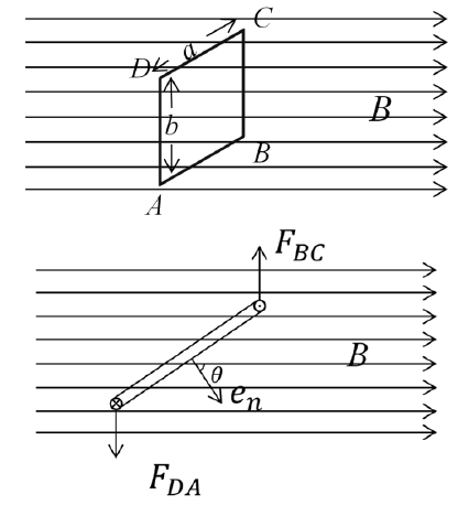
2.1 The magnetic moment of an electric-current coil
Consider a rectangular electric-current coil in an uniform magnetic field, as shown in Fig.1. From Ampere’s law we know the net force on the coil is zero. But the moment of force on the coil is not zero, whose magnitude is given by
| (1) |
Considering the direction, the moment of force takes the form
| (2) |
where is the coil area, is the unit vector of the normal direction of the coil, and the magnetic moment is defined as
| (3) |
It is proved in electromagnetism zhao2018ele that the above two formulas apply to planar coils of arbitrary shape.
2.2 The magnetic moment of a charged lepton as a classical rigid-body
If a charged lepton like a muon is regarded as a charged rigid body, and assuming that its charge density is proportional to the mass density , that is , and thus , where and are the charge and mass of the lepton, respectively. The spin that the lepton carries corresponds to a rotation in classical mechanics. If this charged rigid body rotates around the -axis with an angular velocity , then its magnetic moment can be obtained by an integration:
| (4) | ||||
where is the rotational angular momentum of this rigid body. Writing the above result in vector form, we obtain
| (5) |
If this magnetic moment is intrinsic, then its magnitude will not change, and its potential energy in the magnetic field is
| (6) |
where is the magnetic induction intensity.
Of course, such a classical way cannot correctly describe the property of a charged lepton and Eq. (5) needs to be re-derived from Dirac equation with electromagnetic interaction or from QED.
2.3 The magnetic moment of a charged lepton from Dirac equation
In the following we derive such a potential in Eq.(6) from Dirac equation with electromagnetic interaction zeng2007quantum . A charged lepton is described by a Dirac spinor wave function which satisfies Dirac equation. With electromagnetic interaction, the Dirac equation takes the form
| (7) |
where is the electric potential and is the speed of light. We take but keep for the convenience to make a non-relativistic approximation in the following derivation. For the above equation can reduce to the form in quantum field theory. The relationships between the matrices , and the Dirac are and . In Pauli-Dirac representation, we have
| (8) |
We express the four-component wave function as two two-component wave functions:
| (9) |
where the static energy of the lepton has been separated. Substitute Eq. (9) into Eq. (7), we obtain
| (10) | ||||
| (11) |
In the non-relativistic limit, the terms that do not contain in Eq. (11) can be ignored, and thus we have
| (12) |
Substituting this result into Eq. (10) and taking , we obtain
| (13) |
Using the relation
| (14) |
we can get
| (15) | ||||
Substituting Eq. (15) into Eq. (13), we have
| (16) |
where is the spin of the lepton. Therefore, in non-relativistic approximation,
| (17) |
Now comparing this result with Eq. (6), we obtain
| (18) |
where the factor is called the Landé factor.
2.4 The magnetic moment of a charged lepton from QED at tree level
The potential of a charged lepton with a magnetic moment in magnetic field takes a form in Eq.(6). So the magnetic moment of a charged lepton can be found out from such a potential.
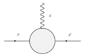
In QED, as depicted in Fig.2, the electromagnetic interaction of a charged lepton takes a form at tree level
| (19) |
where is the four-vector potential of the electromagnetic field, is the magnitude of the electric charge of the charged lepton and is the Dirac algebra representation matrix given by
| (20) |
with being the Pauli matrices.

Since we only consider the influence of the applied magnetic field, we have and
| (21) |
In Weyl representation we obtain the free plane-wave solution of the Dirac equation of a charged lepton (we omit the plane-wave factor for the time being) peskin2018introduction
| (22) |
where is the mass of the charged lepton, and the normalization constant is to make . So we have
| (23) |
From the property of the Pauli matrices
| (24) | |||
| (25) | |||
| (26) |
we obtain
| (27) |
where . Herefater we will not consider the first term which does not contain matrices and thus is irrelevant to spin and magnetic moment. In the second term, and come from and , respectively. Retaining the plane-wave factor , we have
| (28) |
where the total derivative term can be neglected. Since the magnectic potential and the magnetic field are related as
| (29) |
then we have the spin-dependent (SD) interaction
| (30) |
with being the magnetic moment of a charged lepton
| (31) |
and being the spin of a charged lepton (see eq.(3.111) in peskin2018introduction )
| (32) |
2.5 The of a charged lepton from QED beyond tree level
In QED beyond tree level, as shown in Fig.3, the interaction vertex of a charged lepton with electromagnetic field takes the effective form
| (33) |
where is the polarization vector of the electromagnetic field and is an effective form invloving all Lorentz vectors in Fig.3.
The general form of includes , , , and some contractions of the anti-symmetric tensor with the momentums. Utilizing the relations
| (34) | |||
| (35) | |||
| (36) | |||
| (37) |
we can reform not to contain the contrations of matrics or with the momentums. Finally, takes a form
| (38) |
where the factor ensures the corresponding to be dimensionless, and the factor ensures the corresponding to be real so that is hermitian. As the functions of , the coefficients are Lorentz scalars.
Since is a conserved current in QED, we have
| (39) |
which will further restrain the form of . From the relations
| (40) | |||
| (41) | |||
| (42) |
we have
| (43) |
which leads to and . Then takes a form
| (44) |
Further, utilizing the Gordon identities
| (45) | |||
| (46) |
we have
| (47) |
where the renamed coefficients are called form factors.
Since the parameter in the Hamiltonian density will be corrected by the form factors, it is no longer the measured electric charge which needs to be redefined. For this end, we take and then only need to consider . Taking the zero-momentum limit and utilizing
| (48) |
and
| (49) |
we obtain
| (50) |
which means we have a term in the Hamiltonian density:
| (51) |
This term is just the electric potential and thus is the physical charge. So we need to redefine the electric charge to be , which means . This is called the renormalization condition of the electric charge. Therefore, the first term of is .
Since we are concerned primarily with the magnetic moment, we focus on the term. For simplicity we set . In the low energy limit , for only the spatial components need to be considered. On the other hand, since the term already contains the momentums to the first power, we can use the zero-momentum limit of . Also noticing the relation
| (52) |
we have
| (53) |
Compared with eqs.(28-30), this leads to an additional term in the Hamiltonian
| (54) |
Compared with eq.(31), we have
| (55) |
where
| (56) | |||
| (57) |
In the calculation of , we usually need not to derive the whole . We can use the algebra to construct a model-independent projection matrix and then calculate .
Before ending this section, we digress a little to discuss the form of electric dipole moment of a charged lepton. For this end, consider the term in eq.(47) in the low energy limit and set . Then for we only need to cosider . Noticing the relation
| (58) |
we have
| (59) | |||||
where . Compared with the potential of an electric dipole momemnt in an electric field , we obtain the electric dipole moment of a charged lepton
| (60) |
3 The measurement of muon at BNL and Fermilab
So far our discussions on magnetic moment and are applicable to any charged lepton, which in the SM can be an electron, a muon or a tau. If new physics at some high energy scale contributes to , its contribution satisfies
| (61) |
This means that the of a heavier lepton is more sensitive to new physics. Although the tau lepton is heaviest, its liftime is too short and its is very hard to precisely measure. The electron is stable and can be copiously produced, but its mass is too small, about of the muon mass. Overall, among the leptons, the muon is the best probe of new physics.
3.1 A description of the measuring method
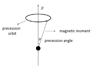
Due to its magnetic moment , an electric-current coil in a magnetic field may have a non-zero moment of force and hence rotate. For a muon, if assumed to be a uniformly charged ball, its spin may lead to a non-zero moment of force which make the spin rotate around the applied magnetic field:
| (62) |
This is called the Larmor precession of a muon, as shown in Fig.4. The angular velocity of the precession is
| (63) |
So we can obtain the value of from the measurement of the muon spin-change angle in a given period of time. The short lifetime (2.2 ) of a muon can be prolonged by its high velocity from special theory of reletivity. On the other hand, technically the moving muons are easier to control than stationary muons. So in experiments the muons are produced in some way and then injected into a storage ring where the spin precessions are measured.
Of course, in experiments the spin changes of the muons are not measured directly. Instead, they are performed via the measurement of its decay products, i.e., the electrons. The technical details are beyond the scope of this review. However, we should note that the measurement mentioned above is discussed assuming the muons to be stationary. In real experiments, the muons are moving in a storage ring. So we need to perform a Lorentz transformation to obtain the formulas in the laboratory frame. The result in the the laboratory frame is given by book:Jegerlehner:2017
| (64) |
where
| (65) | |||
| (66) |
where is the velocity of the muon and . If the magnetic field is precisely perpendicular to the storage ring and the velocity of the muon satisfies
| (67) |
then is called the magic -factor and can be simplified as
| (68) |
3.2 The results of the measurements
The BNL E821 result is BNL:gmuon
| (69) |
The Fermilab result combined with the BNL result is FNAL:gmuon
| (70) |
The SM predition
| (71) |
consists of the following contributions Aoyama:2012wk ; Aoyama:2019ryr ; Czarnecki:2002nt ; Gnendiger:2013pva ; Davier:2017zfy ; Keshavarzi:2018mgv ; Colangelo:2018mtw ; Hoferichter:2019gzf ; Davier:2019can ; Keshavarzi:2019abf ; Kurz:2014wya ; Melnikov:2003xd ; Masjuan:2017tvw ; Colangelo:2017fiz ; Hoferichter:2018kwz ; Gerardin:2019vio ; Bijnens:2019ghy ; Colangelo:2019uex ; Blum:2019ugy ; Colangelo:2014qya
| (72) | |||
| (73) | |||
| (74) | |||
| (75) | |||
| (76) | |||
| (77) |
where the main uncertainties come from the hadronic contributions in HVP and HLBL. The deviation between the experiment and SM is
| (78) |
which is . However, if the lattice simulation result of the hadronic contribution from the BMW group is taken, the deviation between the experiment and SM can be reduced to gm2-lattice .
3.3 The implication for low energy supersymmetry
The deviation between the experiment and the SM prediction for the muon may be a harpinger of new physics beyond the SM. Among the new physics theories, the low energy supersymmetry (SUSY) is the most popular candidate. In SUSY the smuons or muon sneutrino plus electroweakinos (electroweak gauginos and higgsinos) contribute to muon at one loop level, the same level as the SM. For a common sparticle mass , the SUSY contribution to muon can be approximated as Moroi:1995yh
| (79) |
where is the ratio of the vacuum expectation values of the two Higgs doublets. Clearly, to generate the required contribution to explain the muon deviation, a low SUSY mass and a large are favored. Combined with other experimental constraints, such as the dark matter detections and the LHC searches of sparticles, the favored parameter space of SUSY can be specified, which can be of some guidance for the future search of spartilces at the HL-LHC.
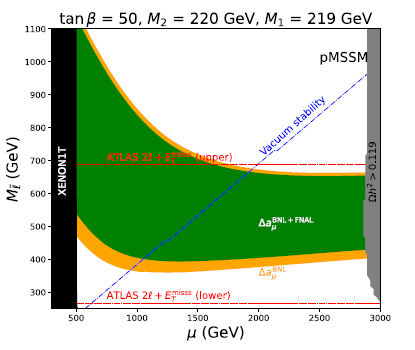
In the low energy effective minimal SUSY model(MSSM) or called phenomenological MSSM(pMSSM). the masses of bino (), winos (), higgsinos () and smuons/sneutrino () are all independent parameters. As shown in Fig. 5 gm2-gutsusy-01 , considering other constraints including the dark matter relic density, the dark matter direct detection, the vacuum stability and the LHC search for sleptons, the survived MSSM parameter space can allow for the explanation of the muon at level gm2-gutsusy-01 ; gm2-mssm-01 ; gm2-mssm-02 ; gm2-mssm-03 ; gm2-mssm-04 ; gm2-mssm-05 ; gm2-mssm-06 ; Iwamoto:2021aaf ; Gu:2021mjd ; Cox:2021gqq .
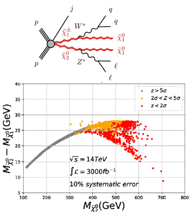
The SUSY explanation of the muon at level requires light electroweakinos and sleptons, which can be most covered at the HL-LHC gm2-mssm-01 ; Aboubrahim:2021ily . For example, in the scenario where the dark matter is bino-like with bino-wino coannihilation to achieve the correct dark matter relic density, the muon at level requires light bino and winos, whose pair production at the LHC can be well probed, as shown in Fig.6.
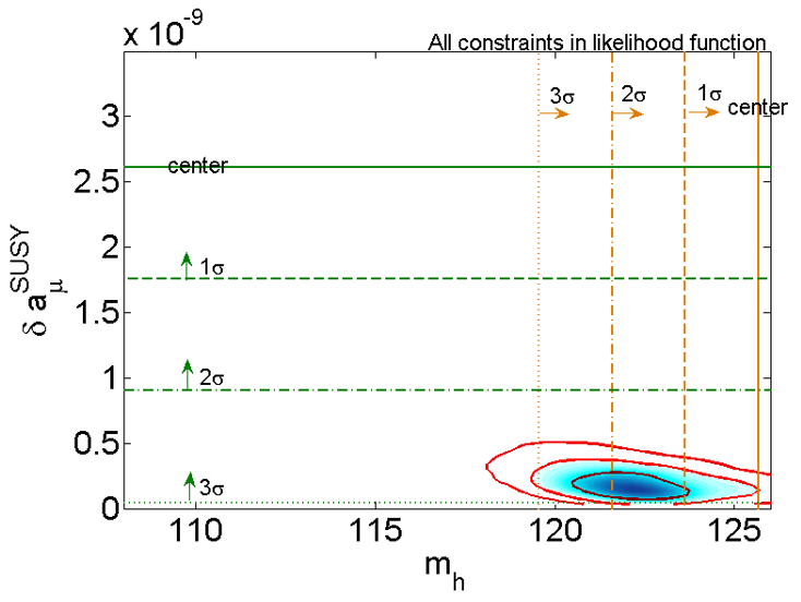
While the muon anomaly can be readily explained in the low energy effective MSSM due to its large number of free soft SUSY-breaking parameters, the explanation is rather challenging in the constrained models with given SUSY breaking mediation mechanisms gm2-gutsusy-01 ; gm2-gutsusy-02 ; gm2-gutsusy-03 ; Han:2020exx ; Lamborn:2021snt ; Yin:2021mls , such as mSUGRA/CMSSM, GMSB and AMSB. In these fancy models we have boundary conditions for the soft SUSY-breaking terms at some high energy scale, e.g., the GUT scale in mSUGRA/CMSSM. Due to the boundary conditions, the soft masses at the weak scale are correlated. To give a 125 GeV SM-like Higgs boson mass, the stop masses must be above TeV scale and the correlated slepton masses cannot be as light as required by the explanation of the muon anomaly. For the mSUGRA/CMSSM, the tension between the 125 GeV SM-like Higgs boson mass and the muon is shown in Fig.7. In order to accomodate a 125 GeV SM-like Higgs boson mass and the muon at level, these models need to improved or extended. For example, one can make colored sparticles much heavier than uncolored sparticles gm2-SUGRA-ext-01 ; gm2-SUGRA-ext-02 ; gm2-SUGRA-ext-03 ; gm2-SUGRA-ext-04 ; gm2-GMSB-AMSB-ext-01 ; gm2-GMSB-AMSB-ext-02 (so stops can be much heavier than sleptons and gluino can be much heavier than electroweakinos at weak scale) or couple the messengers with the Higgs doublets (so the 125 GeV SM-like Higgs boson mass can be achieved without too heavy stops) GMSB-yukawa-higgs .
If we go beyond the minimal framework of SUSY, the accomodation of the 125 GeV SM-like Higgs boson mass and the muon at level may becomes easy. For example, in the next-to-minimal SUSY model (NMSSM) a singlet Higgs field is introduced and hence the 125 GeV SM-like Higgs boson mass can be obtained at tree level without the large effects of heavy stops (the relatively light stops make this model more natural than the MSSM nmssm-mssm ). The explanation of the muon can be achieved in the NMSSM gm2-nmssm-01 ; gm2-nmssm-02 ; gm2-nmssm-03 .
Noe that there have been some attempts to explain the muon together with other physical problems (e.g. the proton radius puzzle Zhu:2021vlz ). Especially, if the value of the fine structure constant measured by the Berkeley experiment berkeley is used, the electron predicted by the SM will also deviate from the experimental value Aoyama:2019ryr ; Hanneke:2008tm . A joint explanation of such an electron anomaly and the muon anomaly is shown to be feasible in SUSY joint-01 ; joint-02 ; joint-03 ; joint-04 ; joint-05 ; Yang:2020bmh . If we further consider the correlation between muon and electron EDM, the CP-phases in SUSY can be stringently constrained cp-phase-01 ; cp-phase-02 . In this review we do not cover various non-SUSY explanations of the or EDM in miscellaneous extensions of the SM, say the 2HDM (see, e.g., Keus:2017ioh ; Wang:2016ggf ; Wang:2018hnw ), the 3-3-1 model (see, e.g., Hue:2021zyw ; Li:2021poy ) and flavor models (see, e.g., Calibbi:2020emz ; Han:2020dwo ; Yin:2021yqy ).
4 Outlook
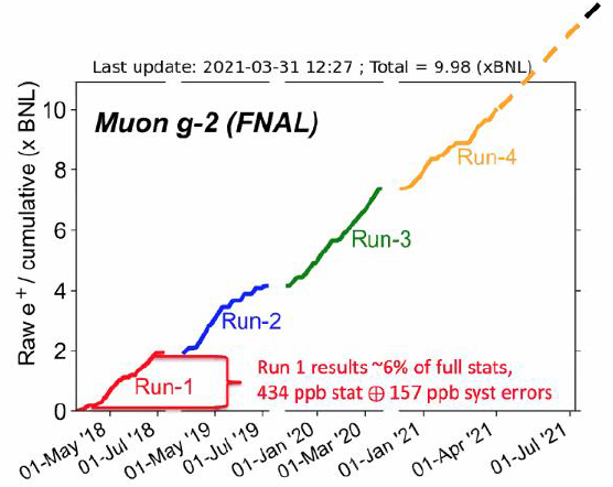
Since the muon may be sensitive to new physics beyond the SM, it will continue playing an important role in the probe of new physics. So the Fermilab experiment on the measurement of the muon has been and will continue to be a focus point in particle physics. So far the result reported by the Fermilab is rather preliminary and only used data of its planned ultimate yield, as shown in Fig.8. In the coming years, Fermilab will continue updating its result amd finally achieve a measuement 4 times as precise as the BNL. If the central measured value and the SM prediction are not changing much, the deviation shown from the final Fermilab result would reach the level. The forthcoming updated results on both the experimental value and the SM calculation improvement (especially from the lattice groups) will bring a huge impact on new physics like the low energy supersymmetry. We just continue to monitor the developments on this front.
Acknowledgements.
This work was supported by the National Natural Science Foundation of China (NNSFC) under grant Nos.11821505 and 12075300, by Peng-Huan-Wu Theoretical Physics Innovation Center (12047503), by the CAS Center for Excellence in Particle Physics (CCEPP), by the CAS Key Research Program of Frontier Sciences, and by a Key R&D Program of Ministry of Science and Technology of China under number 2017YFA0402204.References
- (1) Muon Collaboration collaboration, B. Abi, T. Albahri, S. Al-Kilani, D. Allspach, L. P. Alonzi, A. Anastasi et al., Measurement of the positive muon anomalous magnetic moment to 0.46 ppm, Phys. Rev. Lett. 126 (Apr, 2021) 141801.
- (2) Muon g-2 collaboration, G. W. Bennett et al., Final Report of the Muon E821 Anomalous Magnetic Moment Measurement at BNL, Phys. Rev. D 73 (2006) 072003, [hep-ex/0602035].
- (3) T. Aoyama et al., The anomalous magnetic moment of the muon in the Standard Model, Phys. Rept. 887 (2020) 1–166, [2006.04822].
- (4) K. Zhao and X. Chen, Electromagnetism. Higher Education Press, 4th ed., 2018.
- (5) J. Zeng, Quantum mechanics. Science Press, 4th ed., 2007.
- (6) M. E. Peskin, An introduction to quantum field theory. CRC press, 2018, https://doi.org/10.1201/9780429503559.
- (7) F. Jegerlehner, The Anomalous Magnetic Moment of the Muon. Springer Tracts in Modern Physics volume 274. Springer, second ed., 2017, 10.1007/978-3-319-63577-4.
- (8) T. Aoyama, M. Hayakawa, T. Kinoshita and M. Nio, Complete Tenth-Order QED Contribution to the Muon , Phys. Rev. Lett. 109 (2012) 111808, [1205.5370].
- (9) T. Aoyama, T. Kinoshita and M. Nio, Theory of the Anomalous Magnetic Moment of the Electron, Atoms 7 (2019) 28.
- (10) A. Czarnecki, W. J. Marciano and A. Vainshtein, Refinements in electroweak contributions to the muon anomalous magnetic moment, Phys. Rev. D67 (2003) 073006, [hep-ph/0212229].
- (11) C. Gnendiger, D. Stöckinger and H. Stöckinger-Kim, The electroweak contributions to after the Higgs boson mass measurement, Phys. Rev. D88 (2013) 053005, [1306.5546].
- (12) M. Davier, A. Hoecker, B. Malaescu and Z. Zhang, Reevaluation of the hadronic vacuum polarisation contributions to the Standard Model predictions of the muon and using newest hadronic cross-section data, Eur. Phys. J. C77 (2017) 827, [1706.09436].
- (13) A. Keshavarzi, D. Nomura and T. Teubner, Muon and : a new data-based analysis, Phys. Rev. D97 (2018) 114025, [1802.02995].
- (14) G. Colangelo, M. Hoferichter and P. Stoffer, Two-pion contribution to hadronic vacuum polarization, JHEP 02 (2019) 006, [1810.00007].
- (15) M. Hoferichter, B.-L. Hoid and B. Kubis, Three-pion contribution to hadronic vacuum polarization, JHEP 08 (2019) 137, [1907.01556].
- (16) M. Davier, A. Hoecker, B. Malaescu and Z. Zhang, A new evaluation of the hadronic vacuum polarisation contributions to the muon anomalous magnetic moment and to , Eur. Phys. J. C80 (2020) 241, [1908.00921].
- (17) A. Keshavarzi, D. Nomura and T. Teubner, The of charged leptons, and the hyperfine splitting of muonium, Phys. Rev. D101 (2020) 014029, [1911.00367].
- (18) A. Kurz, T. Liu, P. Marquard and M. Steinhauser, Hadronic contribution to the muon anomalous magnetic moment to next-to-next-to-leading order, Phys. Lett. B734 (2014) 144–147, [1403.6400].
- (19) K. Melnikov and A. Vainshtein, Hadronic light-by-light scattering contribution to the muon anomalous magnetic moment revisited, Phys. Rev. D70 (2004) 113006, [hep-ph/0312226].
- (20) P. Masjuan and P. Sánchez-Puertas, Pseudoscalar-pole contribution to the : a rational approach, Phys. Rev. D95 (2017) 054026, [1701.05829].
- (21) G. Colangelo, M. Hoferichter, M. Procura and P. Stoffer, Dispersion relation for hadronic light-by-light scattering: two-pion contributions, JHEP 04 (2017) 161, [1702.07347].
- (22) M. Hoferichter, B.-L. Hoid, B. Kubis, S. Leupold and S. P. Schneider, Dispersion relation for hadronic light-by-light scattering: pion pole, JHEP 10 (2018) 141, [1808.04823].
- (23) A. Gérardin, H. B. Meyer and A. Nyffeler, Lattice calculation of the pion transition form factor with Wilson quarks, Phys. Rev. D100 (2019) 034520, [1903.09471].
- (24) J. Bijnens, N. Hermansson-Truedsson and A. Rodríguez-Sánchez, Short-distance constraints for the HLbL contribution to the muon anomalous magnetic moment, Phys. Lett. B798 (2019) 134994, [1908.03331].
- (25) G. Colangelo, F. Hagelstein, M. Hoferichter, L. Laub and P. Stoffer, Longitudinal short-distance constraints for the hadronic light-by-light contribution to with large- Regge models, JHEP 03 (2020) 101, [1910.13432].
- (26) T. Blum, N. Christ, M. Hayakawa, T. Izubuchi, L. Jin, C. Jung et al., The hadronic light-by-light scattering contribution to the muon anomalous magnetic moment from lattice QCD, Phys. Rev. Lett. 124 (2020) 132002, [1911.08123].
- (27) G. Colangelo, M. Hoferichter, A. Nyffeler, M. Passera and P. Stoffer, Remarks on higher-order hadronic corrections to the muon , Phys. Lett. B735 (2014) 90–91, [1403.7512].
- (28) S. Borsanyi et al., Leading hadronic contribution to the muon magnetic moment from lattice QCD, Nature 593 (2021) 51–55, [2002.12347].
- (29) T. Moroi, The Muon anomalous magnetic dipole moment in the minimal supersymmetric standard model, Phys. Rev. D 53 (1996) 6565–6575, [hep-ph/9512396].
- (30) F. Wang, L. Wu, Y. Xiao, J. M. Yang and Y. Zhang, GUT-scale constrained SUSY in light of new muon g-2 measurement, Nucl. Phys. B 970 (2021) 115486, [2104.03262].
- (31) M. Abdughani, K.-I. Hikasa, L. Wu, J. M. Yang and J. Zhao, Testing electroweak SUSY for muon 2 and dark matter at the LHC and beyond, JHEP 11 (2019) 095, [1909.07792].
- (32) P. Cox, C. Han and T. T. Yanagida, Muon and dark matter in the minimal supersymmetric standard model, Phys. Rev. D 98 (2018) 055015, [1805.02802].
- (33) P. Athron, C. Balázs, D. H. Jacob, W. Kotlarski, D. Stöckinger and H. Stöckinger-Kim, New physics explanations of in light of the FNAL muon measurement, 2104.03691.
- (34) H. Baer, V. Barger and H. Serce, Anomalous muon magnetic moment, supersymmetry, naturalness, LHC search limits and the landscape, Phys. Lett. B 820 (2021) 136480, [2104.07597].
- (35) W. Altmannshofer, S. A. Gadam, S. Gori and N. Hamer, Explaining with Multi-TeV Sleptons, 2104.08293.
- (36) A. Kobakhidze, M. Talia and L. Wu, Probing the MSSM explanation of the muon g-2 anomaly in dark matter experiments and at a 100 TeV collider, Phys. Rev. D 95 (2017) 055023, [1608.03641].
- (37) S. Iwamoto, T. T. Yanagida and N. Yokozaki, Wino-Higgsino dark matter in the MSSM from the anomaly, 2104.03223.
- (38) Y. Gu, N. Liu, L. Su and D. Wang, Heavy bino and slepton for muon anomaly, Nucl. Phys. B 969 (2021) 115481, [2104.03239].
- (39) P. Cox, C. Han and T. T. Yanagida, Muon and Co-annihilating Dark Matter in the MSSM, 2104.03290.
- (40) A. Aboubrahim, M. Klasen, P. Nath and R. M. Syed, Future searches for susy at the lhc post fermilab , 7, 2021, 2107.06021.
- (41) M. Chakraborti, L. Roszkowski and S. Trojanowski, GUT-constrained supersymmetry and dark matter in light of the new determination, JHEP 05 (2021) 252, [2104.04458].
- (42) A. Aboubrahim, P. Nath and R. M. Syed, Yukawa coupling unification in an SO(10) model consistent with Fermilab result, JHEP 06 (2021) 002, [2104.10114].
- (43) C. Han, M. L. López-Ibáñez, A. Melis, O. Vives, L. Wu and J. M. Yang, LFV and (g-2) in non-universal SUSY models with light higgsinos, JHEP 05 (2020) 102, [2003.06187].
- (44) J. L. Lamborn, T. Li, J. A. Maxin and D. V. Nanopoulos, Resolving the Discrepancy with -(5) Intersecting D-branes, 2108.08084.
- (45) W. Yin, Muon anomaly in anomaly mediation, JHEP 06 (2021) 029, [2104.03259].
- (46) S. Akula and P. Nath, Gluino-driven radiative breaking, Higgs boson mass, muon g-2, and the Higgs diphoton decay in supergravity unification, Phys. Rev. D 87 (2013) 115022, [1304.5526].
- (47) Z. Li, G.-L. Liu, F. Wang, J. M. Yang and Y. Zhang, Gluino-SUGRA scenarios in light of FNAL muon g-2 anomaly, 2106.04466.
- (48) F. Wang, W. Wang and J. M. Yang, Reconcile muon g-2 anomaly with LHC data in SUGRA with generalized gravity mediation, JHEP 06 (2015) 079, [1504.00505].
- (49) F. Wang, K. Wang, J. M. Yang and J. Zhu, Solving the muon g-2 anomaly in CMSSM extension with non-universal gaugino masses, JHEP 12 (2018) 041, [1808.10851].
- (50) F. Wang, W. Wang, J. M. Yang and Y. Zhang, Heavy colored SUSY partners from deflected anomaly mediation, JHEP 07 (2015) 138, [1505.02785].
- (51) F. Wang, J. M. Yang and Y. Zhang, Radiative natural SUSY spectrum from deflected AMSB scenario with messenger-matter interactions, JHEP 04 (2016) 177, [1602.01699].
- (52) Z. Kang, T. Li, T. Liu, C. Tong and J. M. Yang, A Heavy SM-like Higgs and a Light Stop from Yukawa-Deflected Gauge Mediation, Phys. Rev. D 86 (2012) 095020, [1203.2336].
- (53) C. Han, K.-i. Hikasa, L. Wu, J. M. Yang and Y. Zhang, Status of CMSSM in light of current LHC Run-2 and LUX data, Phys. Lett. B 769 (2017) 470–476, [1612.02296].
- (54) J.-J. Cao, Z.-X. Heng, J. M. Yang, Y.-M. Zhang and J.-Y. Zhu, A SM-like Higgs near 125 GeV in low energy SUSY: a comparative study for MSSM and NMSSM, JHEP 03 (2012) 086, [1202.5821].
- (55) X. Ning and F. Wang, Solving the muon g-2 anomaly within the NMSSM from generalized deflected AMSB, JHEP 08 (2017) 089, [1704.05079].
- (56) M. Abdughani, Y.-Z. Fan, L. Feng, Y.-L. S. Tsai, L. Wu and Q. Yuan, A common origin of muon g-2 anomaly, Galaxy Center GeV excess and AMS-02 anti-proton excess in the NMSSM, Sci. Bull. 66 (2021) 1545, [2104.03274].
- (57) J. Cao, J. Lian, Y. Pan, D. Zhang and P. Zhu, Improved measurement and singlino dark matter in -term extended -NMSSM, 2104.03284.
- (58) B. Zhu and X. Liu, Probing the flavor-specific scalar mediator for the muon deviation, the proton radius puzzle and the light dark matter production, 2104.03238.
- (59) R. H. Parker, C. Yu, W. Zhong, B. Estey and H. Müller, Measurement of the fine-structure constant as a test of the Standard Model, Science 360 (2018) 191, [1812.04130].
- (60) D. Hanneke, S. Fogwell and G. Gabrielse, New Measurement of the Electron Magnetic Moment and the Fine Structure Constant, Phys. Rev. Lett. 100 (2008) 120801, [0801.1134].
- (61) S. Li, Y. Xiao and J. M. Yang, Can electron and muon anomalies be jointly explained in SUSY?, 2107.04962.
- (62) B. Dutta and Y. Mimura, Electron with flavor violation in MSSM, Phys. Lett. B 790 (2019) 563–567, [1811.10209].
- (63) M. Badziak and K. Sakurai, Explanation of electron and muon g 2 anomalies in the MSSM, JHEP 10 (2019) 024, [1908.03607].
- (64) M. Endo and W. Yin, Explaining electron and muon anomaly in SUSY without lepton-flavor mixings, JHEP 08 (2019) 122, [1906.08768].
- (65) J. Cao, Y. He, J. Lian, D. Zhang and P. Zhu, Electron and muon anomalous magnetic moments in the inverse seesaw extended NMSSM, Phys. Rev. D 104 (2021) 055009, [2102.11355].
- (66) J.-L. Yang, T.-F. Feng and H.-B. Zhang, Electron and muon in the B-LSSM, J. Phys. G 47 (2020) 055004, [2003.09781].
- (67) S. Li, Y. Xiao and J. M. Yang, Constraining CP-phases in SUSY: an interplay of muon/electron and electron EDM, 2108.00359.
- (68) C. Han, Muon g-2 and CP violation in MSSM, 2104.03292.
- (69) V. Keus, N. Koivunen and K. Tuominen, Singlet scalar and 2HDM extensions of the Standard Model: CP-violation and constraints from and EDM, JHEP 09 (2018) 059, [1712.09613].
- (70) L. Wang, J. M. Yang and Y. Zhang, Probing a pseudoscalar at the LHC in light of and muon g-2 excesses, Nucl. Phys. B 924 (2017) 47–62, [1610.05681].
- (71) L. Wang, J. M. Yang, M. Zhang and Y. Zhang, Revisiting lepton-specific 2HDM in light of muon anomaly, Phys. Lett. B 788 (2019) 519–529, [1809.05857].
- (72) L. T. Hue, K. H. Phan, T. P. Nguyen, H. N. Long and H. T. Hung, An explanation of experimental data of in 3-3-1 models with inverse seesaw neutrinos, 2109.06089.
- (73) T. Li, J. Pei and W. Zhang, Muon Anomalous Magnetic Moment and Higgs Potential Stability in the 331 Model from , 2104.03334.
- (74) L. Calibbi, M. L. López-Ibáñez, A. Melis and O. Vives, Muon and electron and lepton masses in flavor models, JHEP 06 (2020) 087, [2003.06633].
- (75) C. Han, M. L. López-Ibáñez, A. Melis, O. Vives and J. M. Yang, Anomaly-free leptophilic axionlike particle and its flavor violating tests, Phys. Rev. D 103 (2021) 035028, [2007.08834].
- (76) W. Yin, Radiative lepton mass and muon with suppressed lepton flavor and CP violations, 2103.14234.
- (77) Fermilab, “Fermilab Muon .” https://muon-g-2.fnal.gov/.