A Polynomial Time Quantum Algorithm for Exponentially Large Scale Nonlinear Differential Equations via Hamiltonian Simulation

Nonlinear differential equations play a very important role in industry as well as in scientific fields such as physics and mathematics. If quantum computers can be used to analyze such nonlinear differential equations and accelerate the computation, the applications of quantum computers will expand greatly. Besides, the relationship between nonlinear differential equations and machine learning is also attracting attention recently [1]. This could be a new route for the application of quantum computers to the field of machine learning. However, since quantum systems are essentially linear, and hence nontrivial treatment is required to apply quantum computers for solving nonlinear differential equations.

Attempts to linearize nonlinear differential equations have long been studied. The well-known ones are the Carleman linearization [2] and the Koopman-von Neumann linearization [3]. These two linearizations are also closely related to quantum mechanics, and Ref. [4] discusses how to embed and linearize nonlinear differential equations into quantum mechanical systems in a unified framework. In this context, the Carleman linearization maps variables of the system including their higher order nonlinear terms directly to the complex probability amplitudes of a quantum system.

Quantum algorithms for solving nonlinear differential equations using this mapping have been proposed [5]. In Ref. [5], the authors develop the quantum Carleman linearization, a quantum algorithm for dissipative quadratic ordinary differential equations. That algorithm has complexity $O(T^{2}q{\rm poly}(\log T,\log N,\log 1/\epsilon)/\epsilon)$, where $T$ is the evolution time, $\epsilon$ is the allowed error, and $q$ measures decay of the solution. In the quantum Carleman linearization, two infinite dimensional linearizations, the Carleman linearization and the forward Euler method, are applied, and the linearized problem can be solved by the high-precision quantum linear system algorithm (QLSA) [6]. In applying QLSA, the sparsity and the condition number of the matrix are important parameters. The quantum Carleman linearization only inherits the number of terms in the equation as the sparsity. And, two cutoff parameters introduced for those linearizations as accuracy parameters give the bound of the condition number. Further, the complexity depends on the decay $q$. This is inevitable because the linearized differential equations are not Hamiltonian dynamics by applying the Carleman linearization.

On the other hand, the Koopman-von Neumann linearization embeds classical variables via a position state in a continuous variable quantum system. For its discretization, we can employ a number state and its corresponding orthogonal polynomials. The advantage of the latter approach is that such an embedding maps the nonlinear differential equations to Hamiltonian dynamics. While an infinite-dimensional Hilbert space must be truncated by regulating the total particle number, Ref. [7] showed that the truncation error is $O(\eta^{m})$, where $\eta$ is a dimensionless parameter characterizing the strength of the nonlinearity and $m$ is the total particle number. Furthermore, the Hamiltonian simulation [8] was shown to be applied by giving a block encoding, a technique of encoding a matrix as a block of a unitary [9], of the Hamiltonian into which the nonlinear system was embedded. Then, the time complexity was shown to be characterized by the max norm of the matrix embedded in the block encoding, which finally depends on the nonlinear equations.

However, the computational complexity is not fully understood as follows. One problem is that it has been unclear whether or not the mapped Hamiltonian is sparse and whether or not the norm of the Hamiltonian dynamics is conserved. Another and more serious problem is that the nonlinearity $\eta$ was assumed to be sufficiently small, which implicitly depends on the max norm of the mapped Hamiltonian ¹¹1Because of this, the previous version of this paper imposed a condition $\eta T\sim 1$.. Therefore it is still unclear for what kind of nonlinear differential equations can be solved using a quantum computer with what computational complexity in terms of the problem parameters, system size $N$, accuracy $\epsilon$, and simulation time $T$. This motivates to evaluate the computational complexity of solving nonlinear differential equation based on the Koopman-von Neumann linearization more in detail.

To address these difficulties, we present a class of systems of nonlinear ordinary differential equations (ODEs) that can be reducible to the efficient Hamiltonian simulation. (See Fig. 1.) Here, solving a system of ODEs means deriving a quantity described by a multivariate polynomial of finite degree of the variables in the system that have evolved for a finite time. The efficiency means that the time evolution of the system of ODEs can be simulated with a computational complexity of $T{\rm log}(N){\rm polylog}(1/\epsilon)$, where $T$ is the evolution time, $\epsilon$ is the allowed error, and $N$ is the number of variables in the proposed ODEs.

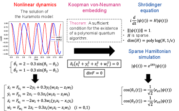
There are two major challenges to solving this problem: first, the norm is not conserved when mapped to Hamiltonian dynamics. The second and the most important one is that the mapped Hamiltonian is not sparse, making it impossible to efficiently apply the Hamiltonian simulation. We show that the proposed ODEs can resolve these two conditions, and they can be solved exponentially efficiently for the number of $N$ variables.

Furthermore, we rigorously evaluate the truncation error in a similar way to Ref. [11], which guarantees that the number of qubits required to achieve an accuracy $\epsilon$ scales $\mathrm{poly}\log(1/\epsilon)$. This compliments the argument given in Ref. [7] and allows us to argue the computational complexity more rigorously.

The proposed ODEs are embedded into Hamiltonian dynamics and applied to the Hamiltonian simulation [9], thus they depends on neither condition number nor the decay of the solution. While the reducible ODEs are a restricted class of systems of ODEs, we claim the broad applications by showing that the proposed ODEs include a wide range of systems of nonlinear ODEs, e.g., classical linear and nonlinear harmonic oscillators, and the short-range Kuramoto model [12]. The short-range Kuramoto model considers locally coupled oscillators, where coupling strength decays with distance, while the classical Kuramoto model describes phase synchronization in globally coupled ones.

\color

blackWe identified the mathematical conditions that allow nonlinear ODEs to be tackled on a quantum computer via the Koopman-von Neumann linearization method, without relying on the Carleman linearization. Based on these conditions, we were able to find the two specific examples mentioned above, although they are toy models. It is expected that this method can be extended to a wider range of practical nonlinear differential equations in the future. Furthermore, while we focused on Hermite polynomials, note that the same approach applies to other orthogonal polynomials.

The rest of this paper is organized as follows. In Sec. II, we briefly review an existing linearization technique of nonlinear ODEs into a quantum system using the position operator embedding. In Sec. III, we introduce a class of nonlinear ODEs and show that the proposed ODEs are embedded into Hamiltonian dynamics. We evaluate the upper bounds of the max norm and the spectral norm of the Hamiltonian associated with the proposed ODEs. Then, we prove the approximation theorem of the cut-offed Hamiltonian dynamics. In Sec. IV, we introduce an approximate representation to reduce the spatial complexity. In Sec. V, we show the algorithm of simulating the proposed ODEs by assuming the sparse access model and the quantum singular value transformation [9]. In Sec. VI, as some applications, we show that the proposed ODEs include classical linear and nonlinear harmonic oscillators, and the short-range Kuramoto model [12]. Section VII is devoted to a conclusion.

In this section, we follow Ref. [4] and introduce a method for embedding a nonlinear system into an infinite dimensional linear system. For simplicity, let us consider one-dimensional case

$\displaystyle\frac{dx}{dt}=F(x),$

(1)

where $F(x)$ is an analytic function. To map Eq. (1) to a linear system, first, we introduce a hermitian operator $\hat{x}$ with the complete set of eigenvectors such that

$\displaystyle\hat{x}\ket{x}=x\ket{x},$

(2)

and

$\displaystyle\braket{n}{x}=w(x)^{1/2}p_{n}(x),n\in\mathbb{Z}_{\geq 0}$

(3)

where $\{\ket{n}\ |\ n\in\mathbb{Z}_{\geq 0}\}$ is the basis set in the occupation number representation and $p_{n}(x)$ is a normalized classical orthogonal polynomial defined by the trinomial recurrence formula

$\displaystyle p_{n+1}(x)=(A_{n}+B_{n}x)p_{n}(x)-C_{n}p_{n-1},n\in\mathbb{Z}_{\geq 0},$

(4)

where $p_{-1}(x)=0$. Using creation and annihilation operators $\hat{a}^{\dagger}$ and $\hat{a}$, i.e.,

$\displaystyle\hat{a}^{\dagger}\ket{n}=\sqrt{n+1}\ket{n+1},\hat{a}\ket{n}=\sqrt{n}\ket{n-1},$

(5)

we have the representation of $\hat{x}=x(\hat{a}^{\dagger},\hat{a})$ as the operator function of $\hat{a}^{\dagger}$ and $\hat{a}$. Second, introducing a hermitian operator $\hat{k}=k(\hat{a}^{\dagger},\hat{a})$ satisfying the commutation relation $[\hat{x},\hat{k}]=iX(\hat{x})$, where $X$ is determined by the choice of the classical orthogonal polynomials, the following vector

$\displaystyle\ket{\tilde{x}(t)}=\exp\Bigl{[}\frac{1}{2}\int_{0}^{t}F^{\prime}(x)d\tau\Bigr{]}\ket{x(t)}$

(6)

satisfies the Shrödinger equation

$\displaystyle i\frac{d}{dt}\ket{\tilde{x}(t)}=\hat{H}\ket{\tilde{x}(t)},$

(7)

where the Hamiltonian $\hat{H}$ is written as

$\displaystyle\hat{H}=\frac{1}{2}\Bigl{(}\hat{k}\frac{F(\hat{x})}{X(\hat{x})}+\frac{F(\hat{x})}{X(\hat{x})}\hat{k}\Bigr{)}.$

(8)

Specifically, if we chose Hermitian polynomial, $\hat{a}^{{\dagger}},\hat{a}$ are the creation and annihilation operators of the harmonic oscillator, and $\hat{k}$ is the momentum operator, which leads $X=1$.

To generalize the above result for a multidimensional case, we focus on an initial value problem described by the following $N$-dimensional ODE

$\displaystyle\frac{dx_{i}}{dt}$

$\displaystyle=$

$\displaystyle F_{i}(\mathbf{x}),\ i\in[N],$

(9)

where $F_{i}(\mathbf{x})$ is a multivariate analytic function and $x_{i}(t)$ is a function of $t$ on the interval $[0,T]$. And let us introduce hermitian operators $\hat{x}_{i}$ with the complete set of eigenvectors $\ket{x_{i}}$. Then, for the nonlinear dynamical system, defining the Hamiltonian $\hat{H}$ as

$\displaystyle\hat{H}=\frac{1}{2}\sum_{i=1}^{N}\Bigl{(}\hat{k}_{i}\frac{F_{i}(\hat{\textbf{x}})}{X(\hat{x}_{i})}+\frac{F_{i}(\hat{\textbf{x}})}{X(\hat{x}_{i})}\hat{k}_{i}\Bigr{)},$

(10)

the Shrödinger equation (7) holds for the following tensor product of states

$\displaystyle\ket{\tilde{\textbf{x}}(t)}$

$\displaystyle=$

$\displaystyle\exp\Bigl{[}\frac{1}{2}\int_{0}^{t}\mathrm{div}F(\mathbf{x})d\tau\Bigr{]}\ket{\textbf{x}(t)},$

(11)

where $\ket{\textbf{x}(t)}:=\bigotimes_{i=1}^{N}\ket{x_{i}(t)}$.

\color

blackThe state $\ket{\tilde{\textbf{x}}(t)}$ in Eq. (11) does not preserve the norm in general. Thus, to avoid the global decaying term, we assume that

$\displaystyle\mathrm{div}F(\mathbf{x})=\sum_{i=1}^{N}\frac{\partial F_{i}(\mathbf{x})}{\partial x_{i}}=0.$

(12)

Furthermore, expanding Eq. (11) in the occupation number representation, we have

$\displaystyle\ket{\textbf{x}(t)}=\bigotimes_{i=1}^{N}\left(w(x_{i})^{\frac{1}{2}}\sum_{n_{i}=0}^{\infty}p_{n_{i}}(x_{i})\ket{n_{i}}\right).$

(13)

The factor $w(\mathbf{x}):=\prod_{i=1}^{N}w(x_{i}(t))$ in Eq. (13) can complicate the representation of desired outputs. Actually, since the output quantity can be obtained as an inner product

$\displaystyle\braket{c\mid\mathbf{x}(t)}=w(\mathbf{x}(t))^{\frac{1}{2}}\sum_{\mathbf{n}:|\mathbf{n}|\leq b}c_{\mathbf{n}}\prod_{i=0}^{N}p_{n_{i}}(x_{i}),$

(14)

where $\ket{c}=\sum_{\mathbf{n}:|\mathbf{n}|\leq b}c_{\mathbf{n}}\ket{\mathbf{n}}$ is an arbitrary state in the Hilbert space restricted to the subspace bounded by the total occupation number $b$, we need to remove $w(\textbf{x}(t))$ from the inner product. In general, the value $w(\textbf{x}(t))$ after time evolution is unknown and its measurement cost is also non trivial. Thus, we assume that $w(\textbf{x}(0))$ is known and we require that

$\displaystyle\dot{w}(\mathbf{x})=\sum_{i=1}^{N}\frac{\partial w(\mathbf{x})}{\partial x_{i}}F_{i}(\mathbf{x})=0.$

(15)

From the above considerations, we present our problem setting for the system of nonlinear differential equations.

\color

blackOn a classical computer, solving Problem 1 requires ${\rm poly}(N)$ overhead in space and time. Our goal here is to solve such a problem in ${\rm polylog}(N)$ qubits and computation time on a quantum computer.

We see that Problem 1 can be divided into three parts. The first part is the preparation of the initial state $\ket{\mathbf{x}(0)}$, which encodes the initial value $\mathbf{x}(0)$. The second part is the efficient Hamiltonian simulation using the Hamiltonian given by Eq. (10). The third part is the evaluation of the output as the inner product $\braket{c\mid\mathbf{x}(T)}$ in Eq. (14).

In this paper, we focus on the second problem and make the assumptions regarding the first and third ones. The assumption for the initial state preparation is given as

The reason for making Assumption 1 is that the distribution of initial values differs for each problem, and whether it is possible to efficiently encode these initial values into a quantum computer depends on whether the data structure of these initial values can be used.

On the other hand, the assumption for the evaluation of the output is given as

To argue the efficient Hamiltonian simulation using the Hamiltonian in Eq. (10), we need to evaluate the Hamiltonian $\hat{H}_{m}$ on the Hilbert space $\mathcal{H}_{m}$ restricted to the subspace bounded by the total occupation number $m$, which is also the accuracy parameter in the algorithmic view point. Therefore, we focus on deriving a sufficiently large scale of the total occupation number $m$ to achieve the required output accuracy $\epsilon$ through the analysis of the simulation error defined in the following.

In the next section, we introduce a restricted class of ODEs that can be solved using the Koopman-von Neumann embedding. By evaluating the error Eq. (17) defined in Eq. (17), we derive the total occupation number $m$ required to achieve the desired accuracy $\epsilon$.

In the rest of the paper, for a given Hilbert space $\mathcal{H}$, a Hamiltonian $\hat{H}$ and a quantum state $\ket{\psi}$, we denote $\mathcal{H}_{m}$, $\hat{H}_{m}$ and $\ket{\psi_{m}}$ as the Hilbert space restricted to the subspace bounded by the total occupation number $m$, the truncated Hamiltonian on $\mathcal{H}_{m}$ and the truncated quantum state in $\mathcal{H}_{m}$, respectively.

We introduce one restricted ODE class solvable with the Koopman-von Neumann embedding, which means that the ODE class is reduced to the evolution equation through Hermite polynomial expansion and satisfies Eq. (12) and Eq. (15).

Note that the other ODE class with terms in which the degree of each variable is two or higher can be reduced to Eq. (18) by introducing dummy variables [7] and considering multiple systems, each identical to the original, including in their initial conditions. In Sec. VI, we show the applicability of the proposed system of ODEs by reducing several systems to it.

The proposed system of ODEs satisfies Eq. (12) trivially, since the term of Eq. (18) does not contain $x_{i}$. It also satisfies Eq. (15) as follows. Considering that the weight function of the Hermite polynomial system is $w(x)=e^{-x^{2}}$, we can check Eq. (15) directly:

	$\displaystyle\dot{w}(\mathbf{x})$	$\displaystyle=$	$\displaystyle\sum_{i=1}^{N}\frac{\partial w(\mathbf{x})}{\partial x_{i}}F_{i}(\mathbf{x})\propto\sum_{i=1}^{N}\sum_{\begin{subarray}{c}p\in\mathcal{S}\\ :i\in p\end{subarray}}\alpha_{p\to i}\prod_{j\in p}x_{j}$		(19)
		$\displaystyle=$	$\displaystyle\sum_{p\in\mathcal{S}}\left(\sum_{i\in p}\alpha_{p\to i}\right)\prod_{j\in p}x_{j}=0,$		(20)

where Eq. (20) is derived as follows. Focusing one $p\in\mathcal{S}$ in Eq. (19), we can see that the term

$\displaystyle\alpha_{p\to i}x_{i}\prod_{j\in p\setminus i}x_{j},$

(21)

appears only once at each $i\in p$ through the sum $\sum_{i=1}^{N}$. Putting these terms together for each $p\in\mathcal{S}$, we obtain Eq. (20).

Clearly, the Hamiltonian corresponding to the proposed ODEs is written by

	$\displaystyle\hat{H}$	$\displaystyle=$	$\displaystyle\sum_{i=1}^{N}\sum_{\begin{subarray}{c}p\in\mathcal{S}\\ :i\in p\end{subarray}}\alpha_{p\to i}\hat{k}_{i}\prod_{j\in p\setminus i}\hat{x}_{j}$		(22)
		$\displaystyle=$	$\displaystyle\sum_{p\in\mathcal{S}}\left(\sum_{i\in p}\alpha_{p\to i}\hat{k}_{i}\prod_{j\in p\setminus i}\hat{x}_{j}\right),$		(23)

where $\hat{x}=(\hat{a}+\hat{a}^{\dagger})/\sqrt{2}$ and $\hat{k}=i(\hat{a}^{\dagger}-\hat{a})/\sqrt{2}$. \colorblack

Then, as stated in Def. 1, we analyze the error given by Eq. (17) that occurs when the initial state is time evolved in the Hilbert space $\mathcal{H}_{m}$ restricted to the subspace bounded by the total occupation number $m$. First, we prove the following technical lemma.

The reason of exponential dependence of the norm on $d$ is as follows. When the system of ODEs is embedded in the sum of local Hamiltonians, the variables are replaced by creation and annihilation operators. Consequently, $d$ corresponds to the maximum degree of creation and annihilation operators in the local Hamiltonian. As a result, the norm is $O(m^{d/2})$.

The spectral norm of the Hamiltonian is crucial for analyzing the error in the time evolution of the state. This is because if the norm is too large, the simulation becomes infeasible, as the approximation error can no longer be guaranteed to converge asymptotically.

Additionally, we introduce a rescaled Hamiltonian

$\displaystyle\hat{H}=\sum_{i=1}^{N}\sum_{\begin{subarray}{c}p\in\mathcal{S}\\ :i\in p\end{subarray}}\frac{\alpha_{p\to i}}{\Delta^{|p|-2}}\hat{k}_{i}\prod_{j\in p\setminus i}\hat{x}_{j},$

(24)

that incorporates a scaling parameter $\Delta$. The rescaling is defined by the transformation $x\to\Delta x$. The rationale behind this rescaling is technical: it is intended to suppress the divergence of inequalities used in error evaluation. Here, we present our main result in the following.

\color

blackWhether the approximation holds depends on the behavior of the higher-order terms when the time evolution operator, defined by the Hamiltonian $\hat{H}_{m}$, is expanded as a series of Hermite polynomials. The total occupation number $m$ ensures a sufficiently large dimension, preventing the loss of information in the output caused by the truncation of the Hilbert space. Theorem 1 demonstrates that these guarantees can be achieved for $m$ and $\Delta$, with scalings of $O\left(\log\left(1/\epsilon\right)\right)$ and $O\left({\rm poly}\log\left(1/\epsilon\right)\right)$, respectively.

As shown later, since we apply the block encoding of $\hat{H}_{m}/||\hat{H}_{m}||_{max}$ to the optimal block-Hamiltonian simulation [9], the effective time required to simulate time $T$ is $||\hat{H}_{m}||_{max}T$ from Lemma 1. More importantly, Theorem 1 shows that if $m$ is sufficiently larger than $b$, an approximated position state $\ket{x}$ in the finite $m$ occupation number representation is sufficient to obtain a degree $b$ polynomial output, which motivates the truncation of the Hilbert space.

The Hamiltonian in the previous section is not efficient in terms of spatial complexity because the input size is proportional to the number of variables $N$. Thus, let us consider truncating the space of the occupation basis such that the total number is limited by some integer $m$ determined by some required precision.

We introduce the following encoding [7]. For any given state $\ket{\mathbf{n}}=\bigotimes_{i=1}^{N}\ket{n_{i}}$ such that $|\textbf{n}|\leq m$,

$\displaystyle\ket{\mathbf{n}}\mapsto\ket{\mathbf{n}_{m}}:=\ket{\underbrace{\overbrace{i_{1}\cdots i_{1}}^{n_{i_{1}}}\overbrace{i_{2}\cdots i_{2}}^{n_{i_{2}}}\cdots\overbrace{i_{l}\cdots i_{l}}^{n_{i_{l}}}}_{m}},$

(26)

where $0\leq i_{1}<\cdots<i_{l}\leq N$, i.e., $\mathbf{n}_{m}$ is all the combinations that take $m$ integers, allowing for duplicates from $N+1$ integers $\{0,1,\cdots,N\}$, in ascending order. Then, the $m$-truncated subspace is defined to be the Hilbert space spanned by the support $\{\ket{\mathbf{n}_{m}}\ |\ |\mathbf{n}|\leq m\}$. The occupation number representation of an initial state

$\displaystyle\ket{\psi(0)}=\sum_{\mathbf{n}}\braket{\mathbf{n}}{\psi(0)}\ket{\mathbf{n}}$

(27)

is encoded into the $m$-truncated subspace such as

$\displaystyle\ket{\psi(0)}\mapsto\ket{\psi_{m}(0)}=\frac{1}{\sqrt{L}}\sum_{\mathbf{n}:|\mathbf{n}|\leq m}\braket{\mathbf{n}}{\psi(0)}\ket{\mathbf{n}_{m}},$

(28)

where $L$ is the normalization constant.

\color

blackFurthermore, in an initial value problem, the occupation number representation of an initial position state $\ket{\mathbf{x}}$ is encoded into the $m$-truncated subspace such as

	$\displaystyle\ket{\mathbf{x}}$	$\displaystyle=$	$\displaystyle\sum_{\mathbf{n}}\braket{\mathbf{n}}{\mathbf{x}}\ket{\mathbf{n}}$		(29)
		$\displaystyle=$	$\displaystyle w(\mathbf{x})^{1/2}\sum_{\mathbf{n}}p_{\mathbf{n}}(\mathbf{x})\ket{\mathbf{n}}$		(30)
	$\displaystyle\mapsto\ket{\mathbf{x}_{m}}$	$\displaystyle=$	$\displaystyle\frac{1}{\sqrt{L}}\sum_{\mathbf{n}:|\mathbf{n}|\leq m}p_{\mathbf{n}}(\mathbf{x})\ket{\mathbf{n}_{m}},$		(31)

where $\ket{\mathbf{n}_{m}}$ is the $m$-truncated basis in Eq. (26), $L$ is the normalized constant ²²2$L$ is a constant thanks to the preservation of $w(\mathbf{x})$, i.e., Eq. (15)., and

$\displaystyle p_{\mathbf{n}}(\mathbf{x})=p_{n_{i_{1}}}(x_{i_{1}})p_{n_{i_{2}}}(x_{i_{2}})\cdots p_{n_{i_{l}}}(x_{i_{l}}).$

(32)

Here, $p_{k}(x)$ is the normalized $k$-th order Hermite polynomial. Clearly, the needed qubit size for these initial states is $m\log N$.

Whether the initial state such as $\ket{\psi_{m}(0)}$ and $\ket{\mathbf{x}_{m}}$ can be efficiently prepared depends on the access models. Thus, instead of Assumption 1, we assume the following initial state preparation.

We briefly discuss the computational complexity of initial state preparation. In general, whether a superposition state with arbitrary coefficients can be efficiently prepared depends on the structure of the coefficients themselves, as it is constrained by the known trade-off between time and space complexities [14, 15].

Therefore, it is generally unreasonable to assume that the initial state can be prepared in logarithmic time. For example, if all the initial values $N$ are independent, the state cannot be prepared in $O(\log N)$ time. However, we expect this assumption to hold for problems of practical importance in applications.

In this section, we argue the Hamiltonian simulation of the mapped Hamiltonian of a system of $N$-dimensional ODEs in Def. 2. We assume that we can access the mapped Hamiltonian matrix through the sparse-access oracles [9].

In this section, we show three examples of ODEs can be reduced to the proposed ODEs in Def. 2. The first two examples are the classical harmonic oscillators, and the undamped and unforced Duffing equations. Recently, a quantum algorithm has been proposed for solving coupled harmonic oscillators, a classical mechanical system, with exponential quantum speedup [16]. While their study can only handle essentially linear systems, we show that our research is capable of addressing nonlinear systems, enabling exponential quantum speedup with respect to the number of variables $N$ in the system.

The other is the Kuramoto model, a simplification of a model introduced by Kuramoto [17] to study huge populations of coupled limit cycle oscillators. We show that the short-range Kuramoto model can be reduced to a system of ODEs in Def. 2, which is one of the promising application candidates for quantum computers, since the treatment of short-range couplings (oscillators embedded in a lattice with nearest-neighbor interactions) presents formidable difficulties both at the analytical and numerical level [12].

References

- Chen et al. [2018] R. T. Q. Chen, Y. Rubanova, J. Bettencourt, and D. K. Duvenaud, in Advances in Neural Information Processing Systems, Vol. 31, edited by S. Bengio, H. Wallach, H. Larochelle, K. Grauman, N. Cesa-Bianchi, and R. Garnett (Curran Associates, Inc., 2018).
- Carleman [1932] T. Carleman, Acta Mathematica 59, 63 (1932).
- Koopman [1931] B. O. Koopman, Proceedings of the National Academy of Sciences 17, 315 (1931).
- Kowalski [1997] K. Kowalski, J. Math. Phys. 38, 2483 (1997).
- Liu et al. [2021] J.-P. Liu, H. Ø. Kolden, H. K. Krovi, N. F. Loureiro, K. Trivisa, and A. M. Childs, Proceedings of the National Academy of Sciences 118, e2026805118 (2021).
- Harrow et al. [2009] A. W. Harrow, A. Hassidim, and S. Lloyd, Physical review letters 103, 150502 (2009).
- Engel et al. [2021] A. Engel, G. Smith, and S. E. Parker, Phys. Plasmas 28, 062305 (2021).
- Low and Chuang [2019] G. H. Low and I. L. Chuang, Quantum 3, 163 (2019).
- Gilyén et al. [2019] A. Gilyén, Y. Su, G. H. Low, and N. Wiebe, in Proceedings of the 51st Annual ACM SIGACT Symposium on Theory of Computing, STOC 2019 (Association for Computing Machinery, New York, NY, USA, 2019) p. 193–204.
- Note [1] Because of this, the previous version of this paper imposed a condition .
- Mizuta and Fujii [2023] K. Mizuta and K. Fujii, Quantum 7, 962 (2023).
- Acebrón et al. [2005] J. A. Acebrón, L. L. Bonilla, C. J. Pérez Vicente, F. Ritort, and R. Spigler, Rev. Mod. Phys. 77, 137 (2005).
- Note [2] is a constant thanks to the preservation of , i.e., Eq. (15).
- Zhang et al. [2022] X.-M. Zhang, T. Li, and X. Yuan, Phys. Rev. Lett. 129, 230504 (2022).
- Sun et al. [2023] X. Sun, G. Tian, S. Yang, P. Yuan, and S. Zhang, IEEE Trans. Comput. Aided Des. Integr. Circuits Syst. 42, 3301 (2023).
- Babbush et al. [2023] R. Babbush, D. W. Berry, R. Kothari, R. D. Somma, and N. Wiebe, Phys. Rev. X 13, 041041 (2023).
- Kuramoto [2012] Y. Kuramoto, Chemical Oscillations, Waves, and Turbulence, Springer Series in Synergetics (Springer Berlin Heidelberg, 2012).
- Hoppensteadt [2000] F. C. Hoppensteadt, Analysis and Simulation of Chaotic Systems, Second Edition (Springer New York, NY, 2000).