These authors contributed equally to this work.
These authors contributed equally to this work.
[2,5]\fnmLijing \surShao
1]\orgdivDepartment of Astronomy, School of Physics, \orgnamePeking University, \orgaddress\streetNo. 5 Yiheyuan Road, \cityBeijing, \postcode100871, \stateBeijing, \countryChina
2]\orgdivKavli Institute for Astronomy and Astrophysics, \orgnamePeking University, \orgaddress\streetNo. 5 Yiheyuan Road, \cityBeijing, \postcode100871, \stateBeijing, \countryChina
3]\orgdivSchool of Physics, \orgnameDalian University of Technology, \orgaddress\streetNo. 2 Linggong Road, \cityDalian, \postcode116024, \stateLiaoning, \countryChina
4]\orgdivInstitute for Gravitational Wave Astronomy, \orgnameHenan Academy of Sciences, \orgaddress\streetNo. 228 Chongshili Road, \cityZhengzhou, \postcode450046, \stateHenan, \countryChina
5]\orgdivNational Astronomical Observatories, \orgnameChinese Academy of Sciences, \orgaddress\street20A Datun Road, \cityBeijing, \postcode100012, \stateBeijing, \countryChina
A practical Bayesian method for gravitational-wave ringdown analysis with multiple modes
Abstract
Gravitational-wave (GW) ringdown signals from black holes (BHs) encode crucial information about the gravitational dynamics in the strong-field regime, which offers unique insights into BH properties. In the future, the improving sensitivity of GW detectors is to enable the extraction of multiple quasi-normal modes (QNMs) from ringdown signals. However, incorporating multiple modes drastically enlarges the parameter space, posing computational challenges to data analysis. Inspired by the -statistic method in the continuous GW searches, we develope an algorithm, dubbed as FIREFLY, for accelerating the ringdown signal analysis. FIREFLY analytically marginalizes the amplitude and phase parameters of QNMs to reduce the computational cost and speed up the full-parameter inference from hours to minutes, while achieving consistent posterior and evidence. The acceleration becomes more significant when more QNMs are considered. Rigorously based on the principle of Bayesian inference and importance sampling, our method is statistically interpretable, flexible in prior choice, and compatible with various advanced sampling techniques, providing a new perspective for accelerating future GW data analysis.
Since the detection of the first gravitational wave (GW) event [1], we have opened new avenues for advancing our understanding of gravity [2, 3], cosmology [4], and astrophysics of compact stars [5, 6]. The final stage of binary black hole (BH) mergers, known as ringdown, describes the progression of remnants to the stable phase, offering a unique opportunity to study BH theories, such as the no-hair theorem [7], the BH area law [8], and properties of the event horizon [9]. A ringdown signal is usually modelled as the superposition of quasi-normal modes (QNMs) of the remnant BH, which can be further divided into spin-weighted spheroidal harmonics with angular indices . Each set of contains a series of overtone modes, indexed by [10, 11]. The extraction and measurement of multiple QNMs provide unparalleled opportunities for studying BHs, known as the BH spectroscopy [12, 11].
The parameter inference of GW signals is mainly based on the Bayes’ theorem,
| (1) |
where in the second equality, we have introduced the terminologies in the Bayesian inference: is called the prior, representing the knowledge of the model parameters before observing the data ; the likelihood is determined by the model, encoding the statistical relation between the parameter and the data; the denominator is called evidence, which can also be regarded as the normalization factor of the numerator according to the law of total probability, . The posterior distribution is the conditional probability of parameters given the data, representing the measurement of parameters after the observation. Therefore, given the prior and the likelihood, the Bayesian inference calculates the posterior distribution according to Eq. (1). However, obtaining an analytical expression (or an efficient numerical formula) of the posterior is usually unfeasible, and a more practical approach is to sample from the posterior distribution and estimate the evidence as an alternative. There are already some techniques to carry out this, such as the Markov-Chain Monte Carlo (MC) [13, 14] and nested sampling methods [15, 16]. These methods partially reduce the difficulty of posterior calculations, but the computational cost is still high when sampling in high-dimensional parameter spaces.
Currently, a typical Bayesian analysis of GW signals can take several hours to days, depending on the number of parameters and the adopted waveform templates. In the future, the next-generation (XG) ground-based GW detectors, such as the Cosmic Explorer (CE) [17, 18] and the Einstein Telescope (ET) [19, 20], will be observing with one order of magnitude higher sensitivity than the current ones, while the near-future space-based detectors, such as the Laser Interferometer Space Antenna (LISA) [21], Taiji [22] and TianQin [23], are expected to detect GWs in the millihertz band. It will become feasible to extract multiple QNMs from ringdown signals [24, 25, 26]. Each QNM component is described by a damping harmonic oscillator consisting of four parameters: amplitude, phase, damping time, and oscillation frequency [27]. In the General Relativity, the latter two parameters are determined by the final mass and spin of the remnant BH. Therefore, adding one QNM mode to ringdown signals increases the dimension of the parameter space by two, and extracting multiple QNMs leads to a challenge in the data analysis. The computational costs are even more prohibitive in tests of no-hair theorem with multiple QNMs, where each mode introduces four free parameters [24, 25, 26].
In this work, we propose an algorithm, named FIREFLY (-statistic Inspired REsampling For anaLYzing GW ringdown signals), to accelerate the Bayesian analysis of parameter estimation. This algorithm is inspired by the -statistic method in the continuous GW searches, which reduces the computational cost by maximizing the likelihood over the extrinsic parameters [28]. In the FIREFLY, the amplitude and phase parameters in the QNMs are analytically marginalized under a specifically chosen prior, reducing the dimensionality of parameter space [29, 30]. Using this auxiliary step, the inference under the target prior can be efficiently performed by importance sampling. In our work, the FIREFLY algorithm reduces the computational time from several hours to a few minutes, while producing consistent posterior distribution and evidence as in the traditional full-parameter Bayesian inference.
FIREFLY does not refine the sampling technique itself, instead, it utilizes the special form of the likelihood and designs more efficient sampling strategies to accelerate the posterior calculation. Compared to the pure -statistic-based methods, which implicitly assume some specific priors [31, 32, 29, 30], FIREFLY is flexible in prior choices because of its efficient importance-sampling design. Compared to current machine-learning-based accelerating algorithms for Bayesian GW data analysis [33, 34, 35, 36], FIREFLY only utilizes the marginalization and resampling techniques in Bayesian analysis, offering a clear and intuitive statistical interpretability. Moreover, any future improvements in the stochastic sampling technique can be incorporated into FIREFLY, further accelerating the inference.
Now we explain the logic of FIREFLY. The recorded GW strain of a ringdown signal is expressed as [27, 30],
| (2) |
where and are reparameterization of the QNM amplitude and phase , while depends on other source parameters, denoted as . Assuming a stationary and Gaussian noise, one finds that the likelihood has a Gaussian form with respect to [30]
| (3) |
where represents the unified notation for , is noise-weighted inner product of the observed data , while , , and are functions of but independent of (see Methods for more details). Based on this Gaussian-form likelihood, FIREFLY aims to accelerate the Bayesian inference, by computing the posterior distribution and evidence given the likelihood (3) and the prior in a target inference problem.
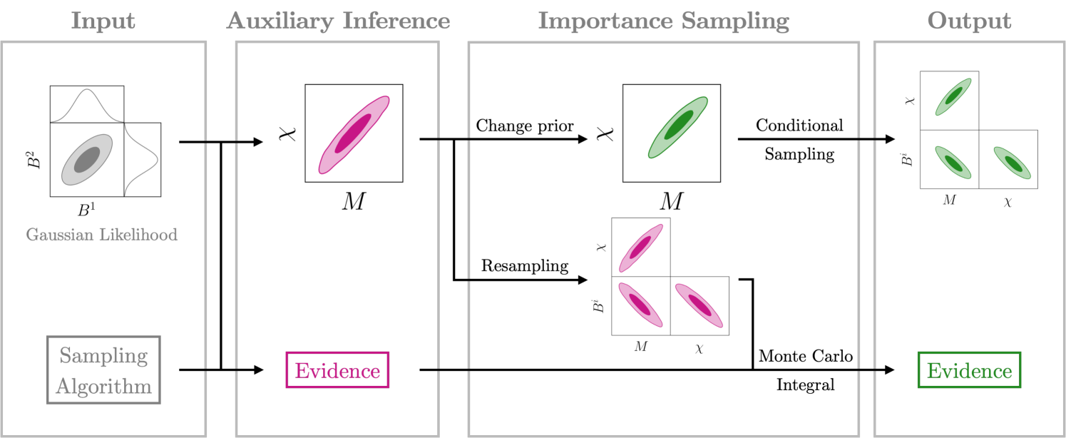
The FIREFLY algorithm mainly composes of two steps: auxiliary inference and importance sampling. In the auxiliary inference, the prior for is chosen as the same as the target inference, denoted as , while the prior for is chosen to be independent of and flat in with a large-enough range, . Note that we use and to distinguish the target and auxiliary priors. Under the auxiliary prior, the QNM parameters can be analytically marginalized, leaving an inference problem only involving . The marginal likelihood for reads
| (4) |
where is the number of QNMs considered in the ringdown waveform. FIREFLY firstly draws samples of with sampling techniques (such as the nested sampling) based on the marginal likelihood and the prior for . These samples are denoted by . The evidence is also obtained by the adopted sampling technique. The auxiliary inference is completed by resampling , which only needs to draw one sample for the -th sample from the Gaussian distribution, ; see Methods for details.
In the second step, FIREFLY performs importance sampling based on the posterior samples, , and the evidence produced by the auxiliary inference. The evidence under the target prior can be estimated by a MC integration, while for the posterior, a direct importance sampling weighted by the prior ratio may lead to large variance [37], especially when the target and auxiliary priors are significantly different (see Methods). Therefore, FIREFLY adopts a two-step importance sampling, dealing with and separately. First, the sample weights for are calculated according to the marginal-posterior ratio for between the target and auxiliary inferences. After the importance resampling for , the sample , assigned to each , is drawn from the conditional posterior,
| (5) |
where the importance-sampling technique is applied once again with a Gaussian proposer.
The output of FIREFLY is the posterior samples and the evidence under the target prior, which is the same as in the full Bayesian inference with all parameters. As we can see, FIREFLY takes advantage of the Gaussian-form likelihood in , and eliminates parameters analytically before applying the time-consuming stochastic sampling techniques. We summarize the workflow of FIREFLY in Fig. 1.
Now we apply FIREFLY to analyze realistic ringdown signals, and compare the results with those from the full Bayesian inference with all parameters, which we refer as the “full-parameter sampling”. To test the performance of FIREFLY in accelerating the extraction of multiple QNMs, we assume the signals are recorded in the triangular-shape ET which consists of three detectors [20]. The data are generated from Numerical Relativity (NR) waveforms of Simulating eXtreme Spacetimes (SXS) catalog [38] and injected into a Gaussian stationary noise corresponding to the ET-D sensitivity.
Specifically, we inject the NR signal SXS:BBH:0305, which is generated by a GW150914-like, non-precessing binary BH (BBH) with a mass ratio of , a detector-frame final mass of , and a dimensionless spin of [38]. The luminosity distance, inclination angle, and reference phase are set to , , and , respectively. The signal-to-noise ratio of ringdown is approximately in the ET, assuming that the signal’s starting time is at its peak amplitude [30]. Usually, for ringdown signals from nearly equal-mass BBHs, one focuses solely on the extraction of QNMs with , while considering different number of overtones [39]. In this work, we consider three scenarios: (i) only the fundamental mode (), (ii) one additional overtone mode (), and (iii) two additional overtone modes (). Since higher-order overtones decay faster and are only potentially significant at earlier times [39], we use the ringdown part from the whole signal at starting times of , and (with the final mass ) after coalescence for , and , respectively.111Here we adopt the geometric units , and corresponds to . In each scenario, it was verified that reasonable adjustments of the starting time do not significantly change our results [30].
When extracting QNMs from the ringdown signal, the variable parameters in the waveform include the right ascension , declination , polarization angle , inclination angle , coalescence time , final mass , and final dimensionless spin , in addition to the QNM parameters . It is also customary to fix the first five parameters based on a more comprehensive study, such as the inspiral-merger-ringdown analysis. For simplicity, we adopt the sky-averaged antenna pattern functions over , , and , and fix and to their injected values. Therefore, in this work only contains the final mass and final spin of the remnant BH, and the full set of variables is , where runs over all QNMs considered in the ringdown signal. Notably, expanding the set of free parameters does not affect the applicability of FIREFLY. In the target inference, we choose flat priors for all parameters, , , and with . In the auxiliary inference, the prior for and remains the same, while the flat prior in corresponds to . We adopt this prior shape for all and , and normalize it in the region of and .
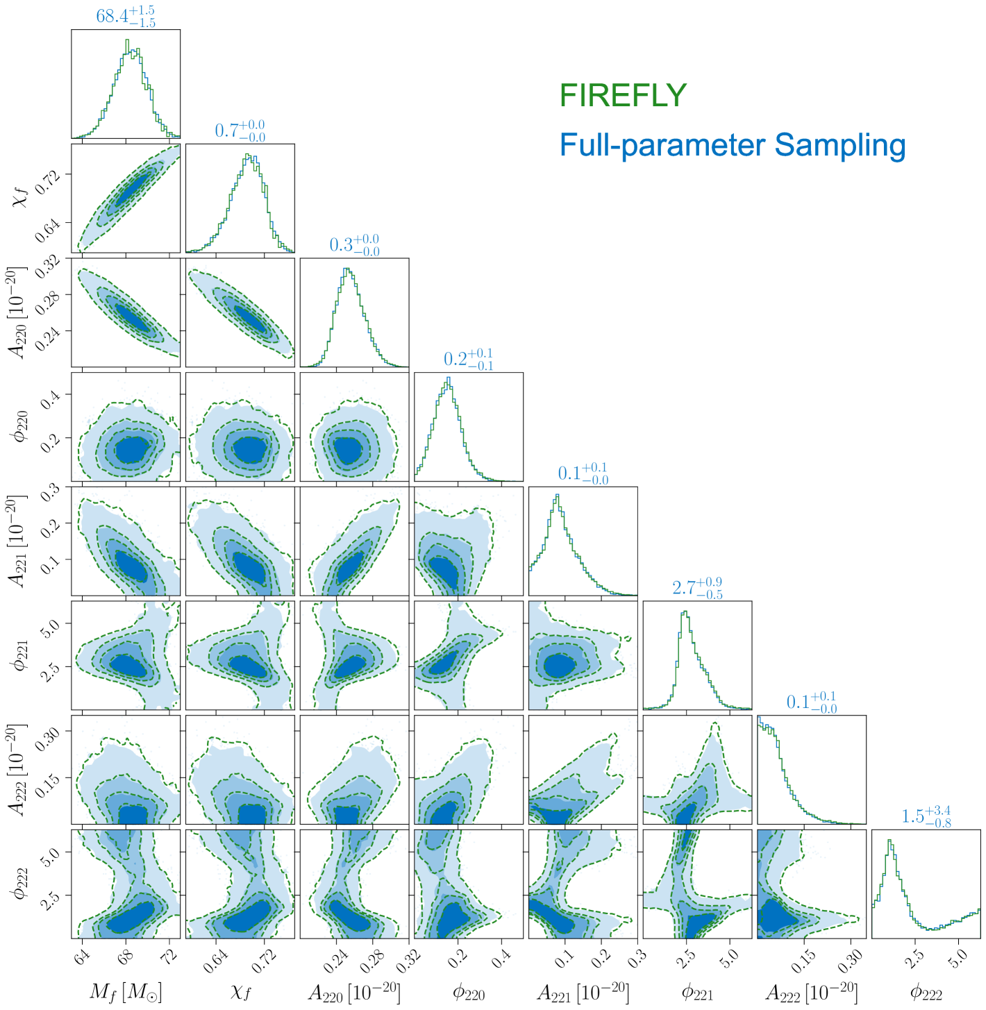
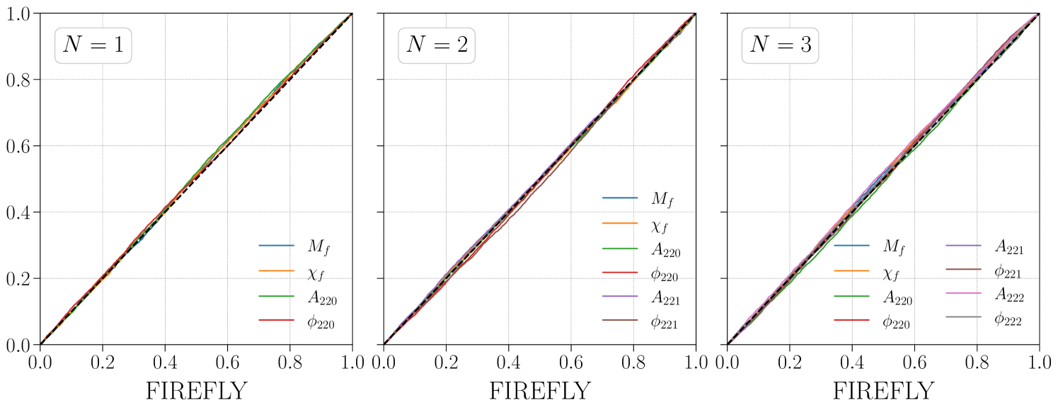
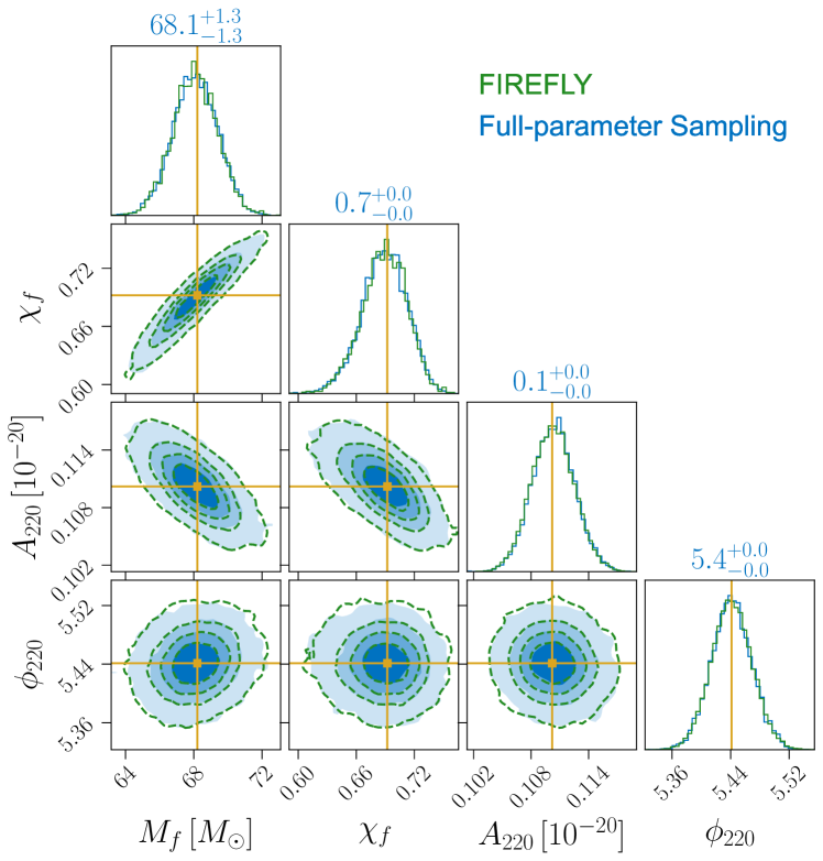
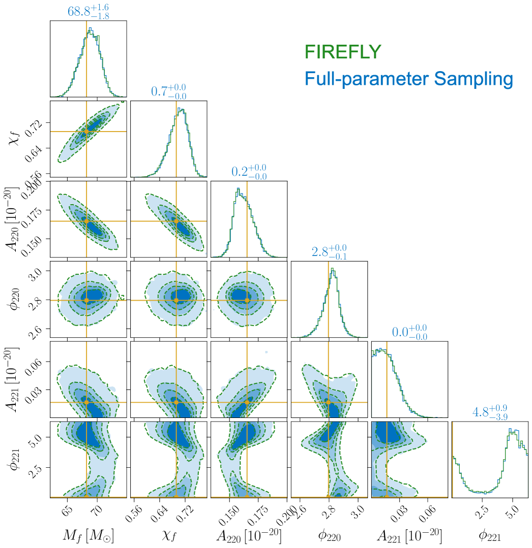
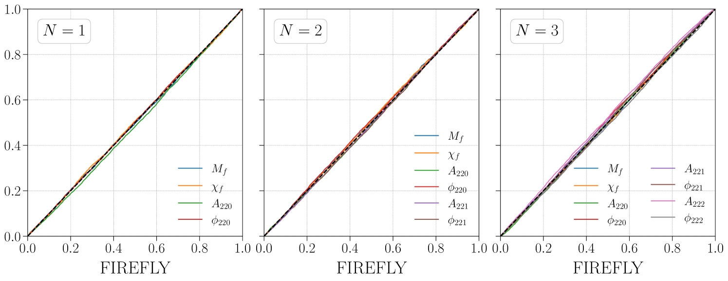
Now we compare the posteriors obtained by FIREFLY and the full-parameter sampling, which directly samples all parameters under the target prior. In both the auxiliary inference and the full-parameter sampling, we use the dynesty [40] sampler to draw samples from the posterior. In all three scenarios, we find that the FIREFLY results closely agree with those from the full-parameter sampling. For concreteness, we show the case in Fig. 2, where the green and blue contours represent the results from the FIREFLY and the full-parameter sampling, respectively. The P-P plots between the one-dimensional marginalized posteriors of the two methods are shown in Fig. 3. We also use the Wasserstein distance to quantitatively verify the consistency between the two methods [41], and find that the average difference of one-dimensional marginal distributions is less than 0.1 standard deviation. The computational times of FIREFLY and the full-parameter sampling are listed in Table 1. In the case, FIREFLY reduces the computational time from several hours to just a few minutes, speeding up by two orders of magnitude.
| FIREFLY | Full-parameter | |||||
|---|---|---|---|---|---|---|
| Sampling | Evidence | IS | Total | Total | -factor | |
| Overtone | 3.2 | |||||
| Overtone | 21.6 | |||||
| Overtone | 103.4 | |||||
| Higher modes | 65.7 | |||||
| \botrule | ||||||
The main reason why FIREFLY significantly accelerates the inference is the analytical marginalization of the QNM amplitude and phase parameters in the auxiliary inference, which eliminates free parameters in the stochastic sampling process. The computational advantage of FIREFLY becomes more pronounced when involving more QNMs in the analysis. Due to the same reason, FIREFLY is fully statistically interpretable, and also compatible with various sampling techniques. Since the majority of the computational time in FIREFLY is spent on the auxiliary inference (see Table 1), one can incorporate the state-of-the-art sampling techniques into FIREFLY, further reducing the computational cost.
FIREFLY also allows flexible prior choices, which is based on the effective two-step importance sampling. In the ringdown signal analysis, different prior choices can significantly affect posteriors, especially when considering multiple QNMs or analyzing weak signals (see Methods). In contrast, the pure -statistic-based methods reduce the number of parameters by analytical maximization, which inherently assumes some specific priors [31, 32, 29, 30]. The flexibility of priors in FIREFLY makes it possible to conduct a more comprehensive analysis when extracting multiple QNMs from ringdown signals. It is also worth noting that changing to a new target prior only requires one to rerun an importance sampling that takes only a few seconds, while the results of auxiliary inference can be reused.
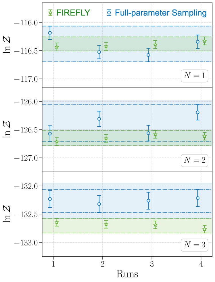
Because of its structure, FIREFLY also gives the evidence estimates, and we compare them with those from the full-parameter sampling in Fig. 4. FIREFLY estimates the evidence with a smaller variance than in the full-parameter sampling. This is because that the uncertainties of the evidence estimation mainly come from the stochastic sampling of the auxiliary inference in FIREFLY, which has fewer free parameters than in the full-parameter sampling. Nevertheless, the evidence estimated by FIREFLY tends to be slightly larger than that of the full-parameter sampling. Similar discrepancies have been reported by other approaches designed to accelerate evidence calculation in GW Bayesian inference [35]. To address this issue, we conduct a comprehensive investigation into the potential uncertainty source and confirm the consistency of the results produced by two methods after considering the additional uncertainties from the insufficient sampling in the full-parameter sampling (see Appendix). Having said that, the relative differences between the two methods are at the level of , so the evidence given by FIREFLY is still largely consistent with the full-parameter sampling.
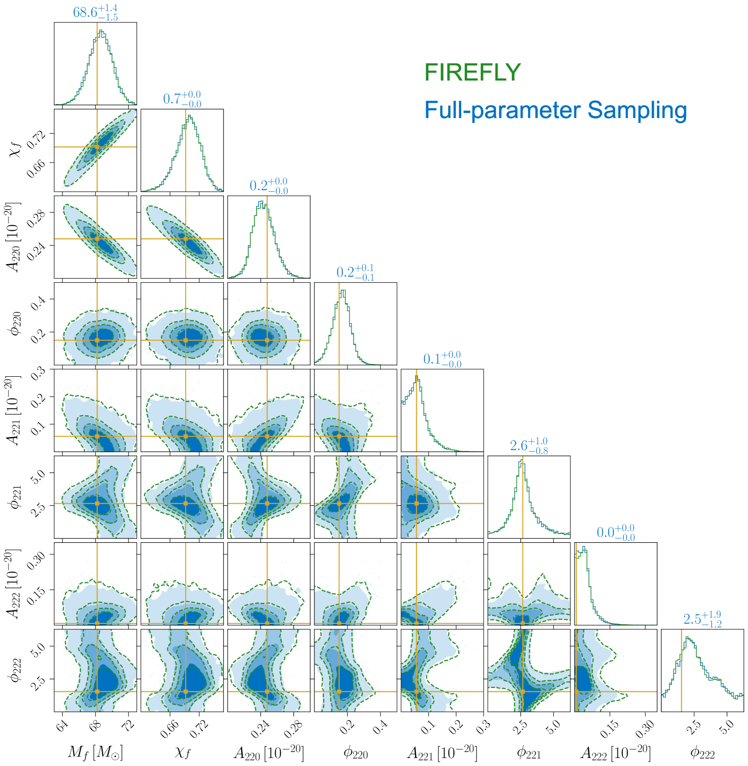
After validating FIREFLY in the parameter estimation of ringdown signals, we now present the extraction of higher modes in the ringdown signal from an asymmetric-mass-ratio BBH system. We inject the NR signal SXS:BBH:0065, which is generated from a non-precessing binary with a mass ratio of , a final redshifted mass of , and a final spin of [38]. The luminosity distance, inclination angle, and reference phase are set to , , and , respectively. We extract four QNMs , , , and from the ringdown signal, at different start times , , , and with .222In the geometric units, corresponds to . The prior for the final mass is chosen to be , while priors of other parameters are the same as those in the previous overtone analysis. The joint posteriors of the final mass and the final spin from FIREFLY and the full-parameter sampling are shown in Fig. 5. FIREFLY achieves close agreement with the full-parameter sampling, while reducing the computational time by about sixty times (see the last row in Table 1).
In this work, we develop the FIREFLY algorithm, which significantly accelerates the analysis of ringdown signals while maintaining nearly indistinguishable posterior and evidence estimates. In the spirit of -statistic, by constructing an auxiliary inference where the QNM amplitudes and phases are analytically marginalized, FIREFLY reduces the computational time by several orders of magnitude, demonstrating its potential to address the challenge of dimensionality curse when extracting multiple QNMs. Also, based on the delicately designed importance-sampling strategy, FIREFLY is highly flexible in prior choices, allowing for a more comprehensive analysis for identifying overtones and higher modes in the ringdown signals. FIREFLY presents a computational paradigm that only leverages the intrinsic structure of the likelihood to accelerate the Bayesian inference, which is fully statistically interpretable, and compatible with any improvements in stochastic sampling techniques. Similar structures are commonly encountered in GW analyses, such as for extreme-mass-ratio inspirals (EMRIs) [42] and GW localization [43]. We hope that the novelty of the FIREFLY algorithm will provide a viable solution to address many more data challenges in future GW data analysis and the beyond.
Methods
Ringdown waveform, likelihood and the . The ringdown signal of a BBH coalescence models the GW waveform from a perturbed BH remnant, and is decomposed into the superposition of QNMs [27],
| (6) | |||
where the damping frequency and damping time are determined by the final mass and the final spin of the remnant, and are the amplitude and phase of the mode . The binary inclination angle is denoted by , while is the azimuthal angle and is usually set to zero. We take the spin-weighted spherical harmonics to approximate the spin-weighted spheroidal harmonics, include the mirror modes, and omit the mode mixing contributions [44, 39]. Combining the waveform model with the antenna pattern function , the recorded GW strain can be expressed as the linear summation in Eq. (2), where the explicit form of is given by
| (7) | ||||
where comprises other parameters in the ringdown waveform except for the QNM amplitude and phase.
In the data analysis of ringdown signals, the likelihood is the conditional probability of the observed data given the model , or equivalently the model parameters and . In this work we use the standard likelihood in the GW data analysis, where the log-likelihood reads [45]
| (8) |
where does not affect the inference, and is fixed to zero. The inner product between two signals, , is defined by,
| (9) |
where the arrow notation indicates that it is a discrete time series sampled from the continuous signal , and is the auto-covariance matrix of the noise at the sampling times, which is determined by the auto-correlation function of the detector noise, or equivalently, the power spectral density of noise. Equation (3) is obtained by formulating the likelihood (8) into a quadratic form with respect to , where and with . The first term in Eq. (3) is called the ,
| (10) |
In addition, if a -detector network is considered, and should be replaced by and respectively, where and are the corresponding quantities in the -th detector. As a short summary, the reparameterization of QNM parameters leads to a Gaussian-form likelihood in , which is the foundation of our FIREFLY algorithm.
Auxiliary inference and the marginal likelihood. In the auxiliary inference, the posterior distribution is
| (11) |
where is the evidence under the auxiliary prior. Formally, one can always marginalize over , and rewrite the marginal posterior of as
| (12) |
with the marginal likelihood [46]
| (13) |
In FIREFLY, the marginal likelihood is analytically given by Eq. (4), since the likelihood is quadratic in and is flat in in our auxiliary prior. Benefiting from this, the marginal likelihood can be evaluated at almost the same speed as for the full likelihood. Noting that Eq. (12) represents an inference problem only involving , FIREFLY applies current stochastic sampling techniques to draw samples based on the marginal likelihood and the prior , and the posterior samples can be regarded as drawn from the marginal posterior , while producing the same evidence as in the full auxiliary inference. To complete the auxiliary inference, we also need to sample , whose conditional posterior given is Gaussian,
| (14) |
Therefore, for each sample , the corresponding is generated by drawing once from the Gaussian distribution . A more detailed description of this resampling technique can be found in the Appendix C of Ref. [47].
Evidence estimation and the two-step importance sampling. Based on the posterior samples and the evidence in the auxiliary inference, FIREFLY calculates the evidence in the target inference by the following formula,
| (15) |
In the second equality, the Bayes’ theorem is applied to rewrite the evidence into an integral involving the posterior and evidence in the auxiliary inference. In the last equality, we approximate the integral by a MC summation with the posterior samples . This technique is widely used to calculate the evidence for hyperparameters in the hierarchical Bayesian inference [47].
As for the posterior samples, FIREFLY first reweighs according to the marginal posterior density ratio of between the target and auxiliary priors, called the marginal importance weight ,
| (16) |
where is the marginal likelihood for under the target prior. Substituting the marginal likelihood in Eq. (4), we find that
| (17) |
The integral in the numerator can be efficiently evaluated by a MC integration with the Gaussian proposer . FIREFLY resamples from the weighted sample set and obtains resampled samples , which are regarded as being drawn from the marginal posterior according to the principle of importance sampling. In the second step, samples of are drawn from the conditional posterior , which can also be performed by the importance-sampling technique. For each , FIREFLY firstly draws samples from , then calculates the weight . The resampled assigned to is generated by a single draw from the weighted sample set . After repeating this procedure for all , samples, denoted as , are obtained, which can be regarded as being drawn from the posterior distribution .
The strategy of two-step importance sampling allows FIREFLY to efficiently resample the posterior samples under the target prior. In principle, one can directly calculate the marginal likelihood by a MC integration, eliminate the dependence on , and sample the posterior of in the target prior. However, this is equivalent to numerically marginalizing in the posterior distribution that requires a MC integration for every likelihood evaluation and is thus computationally expensive. In contrast, FIREFLY executes the MC integration after the sampling and on the samples , making it much more efficient. In the second step, the proposal distribution for is Gaussian, which is also highly efficient for sampling with current algorithms. The two-step strategy again utilizes the Gaussian form of the likelihood in , reducing the computational cost and avoiding the weight divergence in the importance sampling.
The problem of weight divergence. Importance sampling estimates the properties of a target distribution by reweighing samples drawn from a proposal distribution [48]. After drawing samples from , in order to get the samples that follow the target distribution , one computes the importance weights,
| (18) |
and reweighs the samples accordingly. A handy proposal distribution should resemble the target distribution, ensuring importance weight close to one for each sample. If the chosen proposal distribution differs significantly from the target one, it is likely that some samples will have large importance weights , while some others will have weights , leading to a large divergence. The weight divergence refers to a large variance in the importance weights of samples [37]. In this case, the performance of importance sampling deteriorates. Intuitively, a few samples with extremely large weights dominate the importance sampling process, causing significant instability in the MC estimation.
In FIREFLY we need to convert the posterior of the auxiliary inference to the posterior with the target prior, where the importance-sampling proposal and target are the posterior distributions under the auxiliary and target priors. Since they share the same likelihood, the importance weights are proportional to the ratio of the priors. When the target prior is significantly different from the auxiliary one (flat in in FIREFLY), the importance weights can be highly divergent. In this work, the importance weight takes the form of . Therefore, the samples with small will have disproportionately large importance weights, leading to severe weight divergence. A direct importance sampling according to the prior ratio produces unstable distributions with significant variance and spurious structures, as shown in Fig. 6. FIREFLY addresses this issue by performing a two-step importance sampling, avoiding the direct resampling for all parameters. In the first step, FIREFLY resamples with the marginal likelihood ratio , where the problem of weight divergence does not exist. In the second step, one needs to sample in the conditional posterior given , which is the product of the conditional prior and the Gaussian distribution . Benefiting from this specific form of the conditional posterior, one can adopt the importance-sampling technique again to draw samples with a Gaussian proposer. Though weight divergence may still arise with some choices of , the efficient sampling from the Gaussian distribution effectively mitigates this issue. Overall, the two-step importance sampling produces a more stable posterior with smaller variances, which is also closer to the results of full-parameter sampling (cf. Fig. 2).
Simulation configuration and hyperparameters. We perform nested sampling with the Bilby package [49] and the dynesty sampler [40]. The sampler is configured with live points and a termination criterion of . In all samplings, we utilize 16 CPU cores for computation on the FusionServer X6000 V6 equipped with two Intel Xeon Platinum 8358 processors and 256 GB of RAM. The sampling rate of detectors is set to 2048 Hz, which is sufficient for the ringdown signals from BH remnants with mass around .
Apart from the configurations in the auxiliary inference, FIREFLY introduces several additional hyperparameters. The first hyperparameter defines the number of repetitions for computing the evidence with the MC integration. In this work, we set , and calculate the mean and standard deviation of the evidence over 10 repetitions. In the overtone analysis, the contribution to the final uncertainty of the evidence in the MC integration is significantly smaller than that in the auxiliary inference, where the evidence is estimated by the nested sampling.
The second hyperparameter defines the number of samples used to calculate the marginal importance weights with MC integration in the first importance sampling step. Our tests show that provides sufficient accuracy, while increasing further does not lead to significant improvements in the results. We adopt this setting throughout the work.
The third hyperparameter is the number of samples generated in the first importance-sampling step, which is also the total number of posterior samples in FIREFLY. We draw samples based on the importance sampling weights in Eq. (17). Subsequently, the second importance sampling step is then performed to recover the corresponding parameters for each sample.
The fourth hyperparameter describes the number of samples drawn from in the second importance-sampling step. In our configuration, the number of samples obtained from the auxiliary prior is smaller than . Therefore, the effective number of samples for the parameters is fewer than . However, when recovering the parameters for each sample , we fully utilize the special form of the conditional posterior by drawing non-repetitive parameters for each sample . Increasing helps acquire more stable posterior distributions for the parameters .
By construction of the FIREFLY package, the hyperparameters can be adjusted to either speed up the inference or improve the accuracy and stability of the results. Additionally, if auxiliary inference becomes sufficiently efficient, we could explore different importance sampling strategies to generate more compact posterior sample sets. Under the current configuration, FIREFLY already delivers sufficiently fast, stable, and accurate results, but further improvements can be pursued.
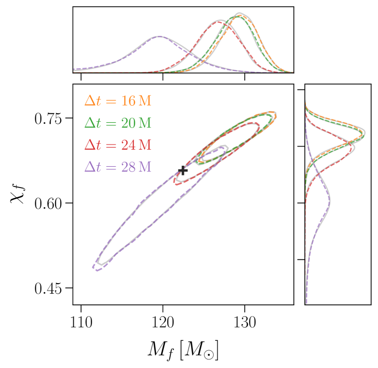
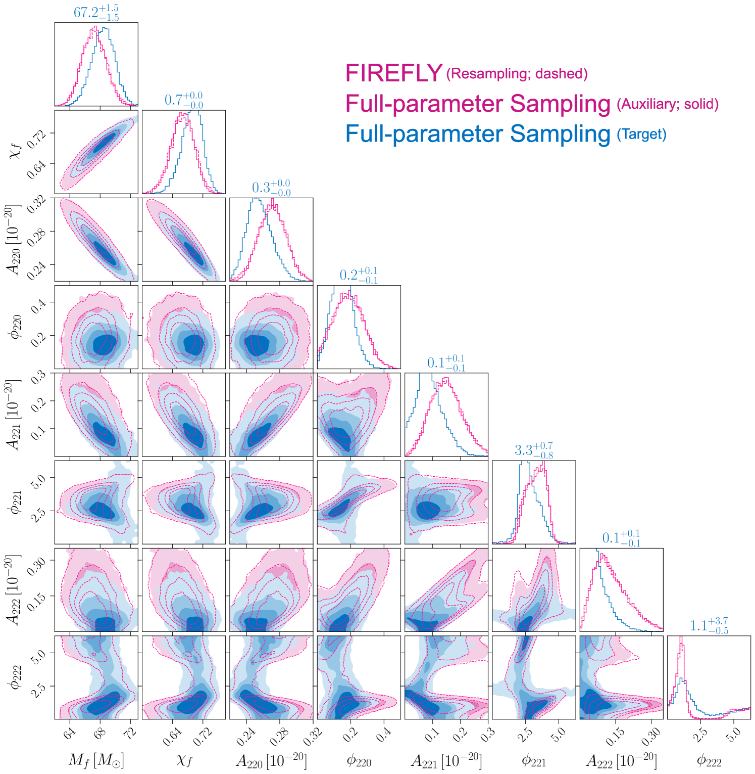
Posterior differences between the auxiliary and target priors. FIREFLY analytically marginalizes the QNM parameters in the auxiliary inference, where the prior is chosen to be flat. The full posterior can be obtained by resampling the QNM parameters based on the posterior samples of . In Fig. 7, we illustrate the result of full-parameter sampling under this auxiliary prior for comparison. For conciseness, we only show the case in overtone analysis. As expected, the posterior distributions from the resampling of in FIREFLY and the full-parameter sampling under the auxiliary prior highly agree with each other. We also illustrate how different priors for affect the posteriors in the ringdown analysis, where noticeable differences are observed in Fig. 7. Compared to the target prior, the posterior of the amplitudes under the auxiliary prior is overestimated, which comes from the flat prior in favoring larger amplitudes. Additionally, since there is a negative correlation between amplitudes and the final mass/spin, the overestimation of amplitudes leads to an underestimation of the mass/spin parameter. For the higher-mode analysis where four QNMs are involved, the posterior differences between the target and auxiliary priors are more significant. Therefore, in the ringdown analysis, different prior choices lead to different posterior distributions, especially extracting multiple QNMs. Advantageously, in FIREFLY the flexibility of the prior selection is achieved by adopting the two-step importance sampling.
Acknowledgements We thank Hyung Won Lee, Hiroyuki Nakano, and Nami Uchikata for comments.
Funding This work was supported by the National Natural Science Foundation of China (123B2043), the Beijing Natural Science Foundation (1242018), the National SKA Program of China (2020SKA0120300), the Max Planck Partner Group Program funded by the Max Planck Society, and the High-performance Computing Platform of Peking University. H.-T. Wang and L. Shao are supported by “the Fundamental Research Funds for the Central Universities” respectively at Dalian University of Technology and Peking University. J. Zhao is supported by the National Natural Science Foundation of China (No. 12405052) and the Startup Research Fund of Henan Academy of Sciences (No. 241841220).
Competing interests The authors declare no competing interests.
Data availability
The data used in this study can be found in the public SXS Gravitational Waveform Database at https://data.black-holes.org/. The data generated and analysed during this study are available from the corresponding author upon reasonable request.
Code availability
The code can be addressed to the corresponding author upon reasonable requests, and will be made publicly available soon.
Author contributions Y.D. and Z.W. contributed equally to the work, on the design and programming of the FIREFLY code, and writing the initial draft of the paper. H.-T.W. contributed to the -statistic-based method, and developed preliminary sampling codes for ringdown analysis in this work. J.Z. contributed to the Bayesian analysis and sampling implementation. L.S. contributed to the design and methodology of FIREFLY, and writing of the paper, and provided supervision and coordination of the whole project. All co-authors discussed the results and provided input to the data analysis and the content of the paper.
Appendix A Zero-noise Injection
In this Appendix, we present the results of FIREFLY in zero-noise injections, where the data are injected according to Eq. (6) and only involving the QNMs to be extracted. We show the test results in the overtone analysis. The source parameters of the injected signals are chosen to be the same as those in the main text, while the amplitudes and phases of each QNM are set to reasonable values based on NR analysis [39], as shown in Table 2. Other configurations such as the priors and hyperparameters are consistent with the overtone analysis in the main text.
| Mode | ||||||
|---|---|---|---|---|---|---|
| – | – | – | – | |||
| – | – | |||||
| \botrule |
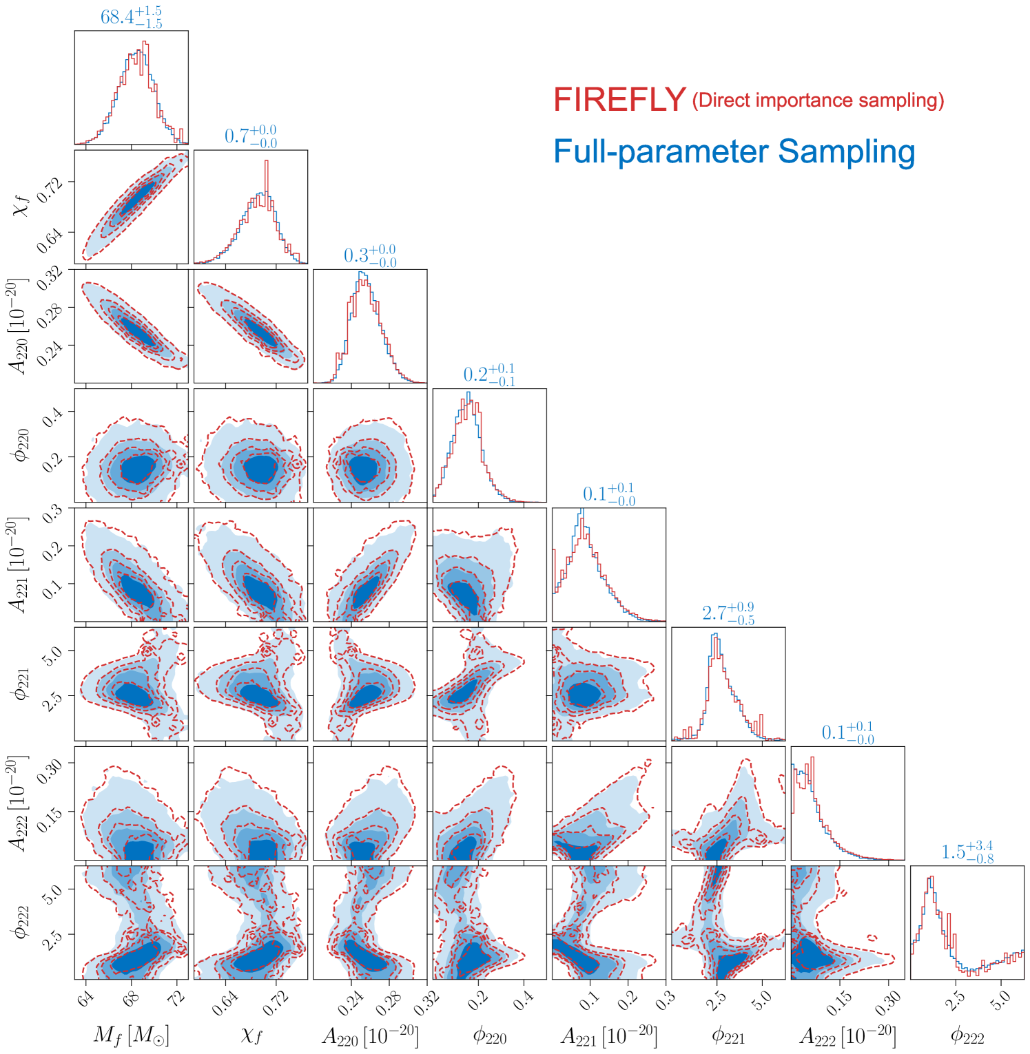
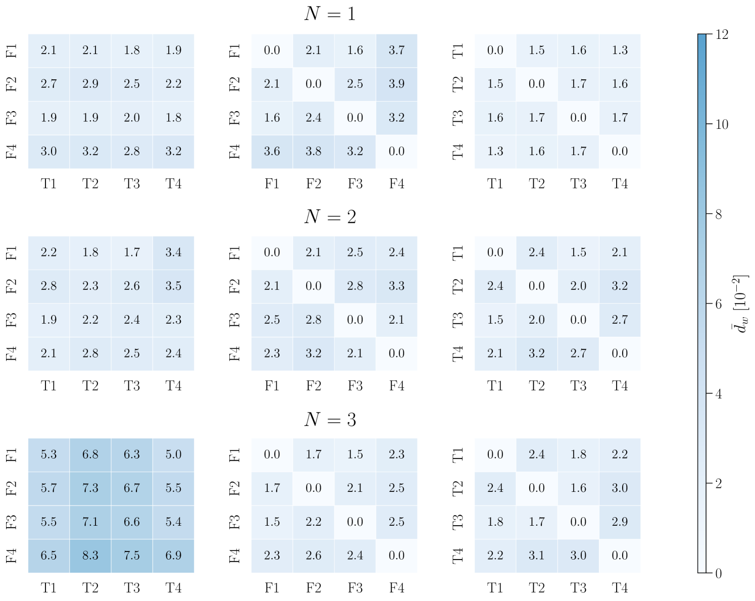
The posteriors given by FIREFLY and the full-parameter sampling are shown in Figs. 8–10, corresponding to the cases of , , and , respectively. While all results of the two methods are highly consistent visually with each other and the injection values, we further quantify the differences between the two methods using the P-P plot and the Wasserstein distance. In Fig. 11, we depict the P-P plot of the one-dimensional marginal posteriors between the two methods in all three scenarios. The Wasserstein distance, also known as the Earth-Mover’s distance, measures the minimum cost of transforming one distribution into another, providing a robust metric for comparing distributions [41]. We compute the Wasserstein distance between each pair of the one-dimensional marginal posteriors from the two methods, and normalize it with the standard deviation of the one-dimensional posterior distribution in the full-parameter sampling. The normalized Wasserstein distances are further averaged over all parameters, providing a single, average, normalized Wasserstein distance , shown in Fig. 12. For each model, the analysis is performed independently four times for both FIREFLY and the full-parameter sampling, allowing for a comparison between the two methods as well as their internal variability. In the cases of and , the differences between the two methods are close to the internal fluctuations of each method, which irrefutably demonstrates the accuracy of FIREFLY. In the case of , the difference between the two methods is slightly larger than the internal fluctuations, but remains at a relatively low level with , indicating that the average difference between the one-dimensional marginal distributions of the two methods is less than 0.1 standard deviation.
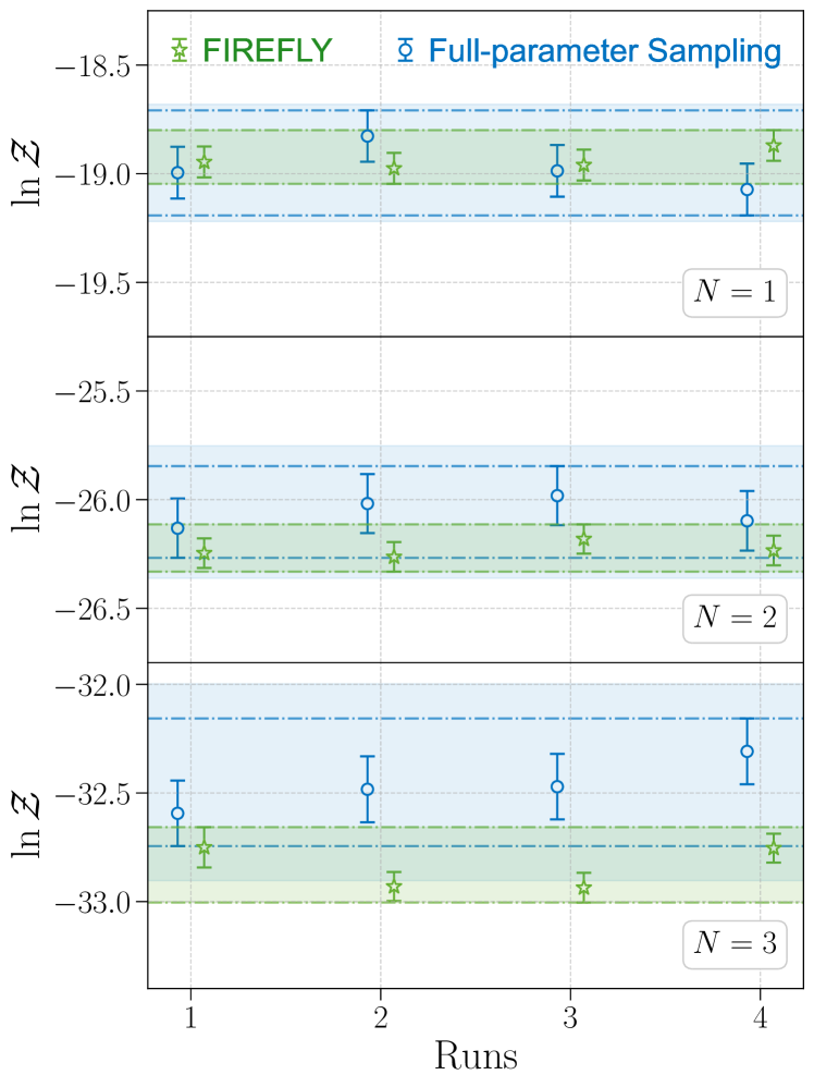
The evidences in different scenarios are also calculated by FIREFLY and the full-parameter sampling. Same as in the main text, we conduct four independent trials for each scenario, and show the results in Fig. 13. The dash-dotted lines represent the upper and lower bounds of the evidence by taking the union of the ranges from the four independent trials. For the full-parameter sampling, we further consider the uncertainties due to insufficient sampling in the QNM parameters. We perform the following numerical experiments to estimate it. First, if and are fixed, then has a Gaussian form in . In the auxiliary inference, we analytically marginalize and obtain the marginal likelihood. In the full-parameter sampling, is treated as the same as and sampled. We find that the nested sampling method tends to overestimate the marginal likelihood in the numerically stochastic sampling of . To quantify this bias, we fix and at their injected values, and compute the Gaussian integration in both analytically and with the nested sampling method. The difference between the two results can be regarded as the bias led by insufficient sampling in , shown in Fig. 14. For the higher-dimensional cases of and , the nested sampling tends to produce overestimated values, which partially explains the small evidence discrepancy between the two methods discussed in the main text. Without further investigation, in this work we simply treat the bias as an additional uncertainty in the full-parameter sampling, and combine it with the evidence uncertainty given by the nested-sampling algorithm. This finally leads to a more conservative estimation of the evidence.
References
- \bibcommenthead
- Abbott et al. [2016a] Abbott, B.P., et al.: Observation of Gravitational Waves from a Binary Black Hole Merger. Phys. Rev. Lett. 116(6), 061102 (2016) https://doi.org/10.1103/PhysRevLett.116.061102 arXiv:1602.03837 [gr-qc]
- Abbott et al. [2016b] Abbott, B.P., et al.: Tests of general relativity with GW150914. Phys. Rev. Lett. 116(22), 221101 (2016) https://doi.org/10.1103/PhysRevLett.116.221101 arXiv:1602.03841 [gr-qc]. [Erratum: Phys.Rev.Lett. 121, 129902 (2018)]
- Abbott et al. [2021] Abbott, R., et al.: Tests of General Relativity with GWTC-3 (2021) arXiv:2112.06861 [gr-qc]
- Abbott et al. [2017] Abbott, B.P., et al.: A gravitational-wave standard siren measurement of the Hubble constant. Nature 551(7678), 85–88 (2017) https://doi.org/10.1038/nature24471 arXiv:1710.05835 [astro-ph.CO]
- Abbott et al. [2018] Abbott, B.P., et al.: GW170817: Measurements of neutron star radii and equation of state. Phys. Rev. Lett. 121(16), 161101 (2018) https://doi.org/10.1103/PhysRevLett.121.161101 arXiv:1805.11581 [gr-qc]
- Abbott et al. [2023] Abbott, R., et al.: Population of Merging Compact Binaries Inferred Using Gravitational Waves through GWTC-3. Phys. Rev. X 13(1), 011048 (2023) https://doi.org/10.1103/PhysRevX.13.011048 arXiv:2111.03634 [astro-ph.HE]
- Isi et al. [2019] Isi, M., Giesler, M., Farr, W.M., Scheel, M.A., Teukolsky, S.A.: Testing the no-hair theorem with GW150914. Phys. Rev. Lett. 123(11), 111102 (2019) https://doi.org/10.1103/PhysRevLett.123.111102 arXiv:1905.00869 [gr-qc]
- Isi et al. [2021] Isi, M., Farr, W.M., Giesler, M., Scheel, M.A., Teukolsky, S.A.: Testing the Black-Hole Area Law with GW150914. Phys. Rev. Lett. 127(1), 011103 (2021) https://doi.org/10.1103/PhysRevLett.127.011103 arXiv:2012.04486 [gr-qc]
- Cardoso et al. [2016] Cardoso, V., Franzin, E., Pani, P.: Is the gravitational-wave ringdown a probe of the event horizon? Phys. Rev. Lett. 116(17), 171101 (2016) https://doi.org/10.1103/PhysRevLett.116.171101 arXiv:1602.07309 [gr-qc]. [Erratum: Phys.Rev.Lett. 117, 089902 (2016)]
- Teukolsky [1973] Teukolsky, S.A.: Perturbations of a rotating black hole. 1. Fundamental equations for gravitational electromagnetic and neutrino field perturbations. Astrophys. J. 185, 635–647 (1973) https://doi.org/10.1086/152444
- Berti et al. [2007] Berti, E., Cardoso, J., Cardoso, V., Cavaglia, M.: Matched-filtering and parameter estimation of ringdown waveforms. Phys. Rev. D 76, 104044 (2007) https://doi.org/10.1103/PhysRevD.76.104044 arXiv:0707.1202 [gr-qc]
- Dreyer et al. [2004] Dreyer, O., Kelly, B.J., Krishnan, B., Finn, L.S., Garrison, D., Lopez-Aleman, R.: Black hole spectroscopy: Testing general relativity through gravitational wave observations. Class. Quant. Grav. 21, 787–804 (2004) https://doi.org/10.1088/0264-9381/21/4/003 arXiv:gr-qc/0309007
- Christensen and Meyer [1998] Christensen, N., Meyer, R.: Markov chain Monte Carlo methods for Bayesian gravitational radiation data analysis. Phys. Rev. D 58, 082001 (1998) https://doi.org/10.1103/PhysRevD.58.082001
- Sharma [2017] Sharma, S.: Markov Chain Monte Carlo Methods for Bayesian Data Analysis in Astronomy. Ann. Rev. Astron. Astrophys. 55, 213–259 (2017) https://doi.org/10.1146/annurev-astro-082214-122339 arXiv:1706.01629 [astro-ph.IM]
- Skilling [2004] Skilling, J.: Nested Sampling. AIP Conf. Proc. 735(1), 395 (2004) https://doi.org/10.1063/1.1835238
- Skilling [2006] Skilling, J.: Nested sampling for general Bayesian computation. Bayesian Analysis 1(4), 833–859 (2006) https://doi.org/10.1214/06-BA127
- Reitze et al. [2019a] Reitze, D., et al.: Cosmic Explorer: The U.S. Contribution to Gravitational-Wave Astronomy beyond LIGO. Bull. Am. Astron. Soc. 51(7), 035 (2019) arXiv:1907.04833 [astro-ph.IM]
- Reitze et al. [2019b] Reitze, D., et al.: The US Program in Ground-Based Gravitational Wave Science: Contribution from the LIGO Laboratory. Bull. Am. Astron. Soc. 51, 141 (2019) arXiv:1903.04615 [astro-ph.IM]
- Punturo et al. [2010] Punturo, M., et al.: The Einstein Telescope: A third-generation gravitational wave observatory. Class. Quant. Grav. 27, 194002 (2010) https://doi.org/10.1088/0264-9381/27/19/194002
- Hild et al. [2011] Hild, S., et al.: Sensitivity Studies for Third-Generation Gravitational Wave Observatories. Class. Quant. Grav. 28, 094013 (2011) https://doi.org/10.1088/0264-9381/28/9/094013 arXiv:1012.0908 [gr-qc]
- Amaro-Seoane et al. [2017] Amaro-Seoane, P., et al.: Laser Interferometer Space Antenna. e-prints (2017) https://doi.org/10.48550/arXiv.1702.00786 [astro-ph.IM]
- Hu and Wu [2017] Hu, W.-R., Wu, Y.-L.: The Taiji Program in Space for gravitational wave physics and the nature of gravity. Natl. Sci. Rev. 4(5), 685–686 (2017) https://doi.org/10.1093/nsr/nwx116
- Luo et al. [2016] Luo, J., et al.: TianQin: a space-borne gravitational wave detector. Class. Quant. Grav. 33(3), 035010 (2016) https://doi.org/10.1088/0264-9381/33/3/035010 arXiv:1512.02076 [astro-ph.IM]
- Bhagwat et al. [2022] Bhagwat, S., Pacilio, C., Barausse, E., Pani, P.: Landscape of massive black-hole spectroscopy with LISA and the Einstein Telescope. Phys. Rev. D 105(12), 124063 (2022) https://doi.org/10.1103/PhysRevD.105.124063 arXiv:2201.00023 [gr-qc]
- Bhagwat et al. [2023] Bhagwat, S., Pacilio, C., Pani, P., Mapelli, M.: Landscape of stellar-mass black-hole spectroscopy with third-generation gravitational-wave detectors. Phys. Rev. D 108(4), 043019 (2023) https://doi.org/10.1103/PhysRevD.108.043019 arXiv:2304.02283 [gr-qc]
- Pitte et al. [2024] Pitte, C., Baghi, Q., Besançon, M., Petiteau, A.: Exploring tests of the no-hair theorem with LISA. Phys. Rev. D 110(10), 104003 (2024) https://doi.org/10.1103/PhysRevD.110.104003 arXiv:2406.14552 [gr-qc]
- Berti et al. [2009] Berti, E., Cardoso, V., Starinets, A.O.: Quasinormal modes of black holes and black branes. Class. Quant. Grav. 26, 163001 (2009) https://doi.org/10.1088/0264-9381/26/16/163001 arXiv:0905.2975 [gr-qc]
- Jaranowski et al. [1998] Jaranowski, P., Krolak, A., Schutz, B.F.: Data analysis of gravitational - wave signals from spinning neutron stars. 1. The Signal and its detection. Phys. Rev. D 58, 063001 (1998) https://doi.org/10.1103/PhysRevD.58.063001 arXiv:gr-qc/9804014
- Ashok et al. [2024] Ashok, A., Covas, P.B., Prix, R., Papa, M.A.: Bayesian F-statistic-based parameter estimation of continuous gravitational waves from known pulsars. Phys. Rev. D 109(10), 104002 (2024) https://doi.org/10.1103/PhysRevD.109.104002 arXiv:2401.17025 [gr-qc]
- Wang et al. [2024] Wang, H.-T., Yim, G., Chen, X., Shao, L.: Gravitational Wave Ringdown Analysis Using the F -statistic. Astrophys. J. 974(2), 230 (2024) https://doi.org/10.3847/1538-4357/ad7096 arXiv:2409.00970 [gr-qc]
- Prix and Krishnan [2009] Prix, R., Krishnan, B.: Targeted search for continuous gravitational waves: Bayesian versus maximum-likelihood statistics. Class. Quant. Grav. 26, 204013 (2009) https://doi.org/10.1088/0264-9381/26/20/204013 arXiv:0907.2569 [gr-qc]
- [32] Prix, R.: Bayesian QNM search on black hole ringdown modes (applied to GW150914). LIGO Document, https://dcc.ligo.org/LIGO-T1500618/public
- Gabbard et al. [2022] Gabbard, H., Messenger, C., Heng, I.S., Tonolini, F., Murray-Smith, R.: Bayesian parameter estimation using conditional variational autoencoders for gravitational-wave astronomy. Nature Phys. 18(1), 112–117 (2022) https://doi.org/10.1038/s41567-021-01425-7 arXiv:1909.06296 [astro-ph.IM]
- Dax et al. [2021] Dax, M., Green, S.R., Gair, J., Macke, J.H., Buonanno, A., Schölkopf, B.: Real-Time Gravitational Wave Science with Neural Posterior Estimation. Phys. Rev. Lett. 127(24), 241103 (2021) https://doi.org/10.1103/PhysRevLett.127.241103 arXiv:2106.12594 [gr-qc]
- Dax et al. [2023] Dax, M., Green, S.R., Gair, J., Pürrer, M., Wildberger, J., Macke, J.H., Buonanno, A., Schölkopf, B.: Neural Importance Sampling for Rapid and Reliable Gravitational-Wave Inference. Phys. Rev. Lett. 130(17), 171403 (2023) https://doi.org/10.1103/PhysRevLett.130.171403 arXiv:2210.05686 [gr-qc]
- Pacilio et al. [2024] Pacilio, C., Bhagwat, S., Cotesta, R.: Simulation-based inference of black hole ringdowns in the time domain. Phys. Rev. D 110(8), 083010 (2024) https://doi.org/10.1103/PhysRevD.110.083010 arXiv:2404.11373 [gr-qc]
- [37] Robert, C.P., Casella, G.: Monte carlo statistical methods. Springer (2004), https://link.springer.com/book/10.1007/978-1-4757-4145-2
- Boyle et al. [2019] Boyle, M., et al.: The SXS Collaboration catalog of binary black hole simulations. Class. Quant. Grav. 36(19), 195006 (2019) https://doi.org/10.1088/1361-6382/ab34e2 arXiv:1904.04831 [gr-qc]
- Giesler et al. [2019] Giesler, M., Isi, M., Scheel, M.A., Teukolsky, S.: Black Hole Ringdown: The Importance of Overtones. Phys. Rev. X 9(4), 041060 (2019) https://doi.org/%****␣sn-article.bbl␣Line␣675␣****10.1103/PhysRevX.9.041060 arXiv:1903.08284 [gr-qc]
- Higson et al. [2019] Higson, E., Handley, W., Hobson, M., Lasenby, A.: Dynamic nested sampling: an improved algorithm for parameter estimation and evidence calculation. Statistics and Computing 29(5), 891 (2019) https://doi.org/10.1007/s11222-018-9844-0
- Peyré and Cuturi [2019] Peyré, G., Cuturi, M.: Computational optimal transport: With applications to data science. Foundations and Trends in Machine Learning 11(5-6), 355–607 (2019) https://doi.org/10.1561/2200000073
- Wang et al. [2012] Wang, Y., Shang, Y., Babak, S.: EMRI data analysis with a phenomenological waveform. Phys. Rev. D 86, 104050 (2012) https://doi.org/10.1103/PhysRevD.86.104050 arXiv:1207.4956 [gr-qc]
- Hu and Veitch [2023] Hu, Q., Veitch, J.: Rapid Premerger Localization of Binary Neutron Stars in Third-generation Gravitational-wave Detectors. Astrophys. J. Lett. 958(2), 43 (2023) https://doi.org/10.3847/2041-8213/ad0ed4 arXiv:2309.00970 [gr-qc]
- Berti and Klein [2014] Berti, E., Klein, A.: Mixing of spherical and spheroidal modes in perturbed Kerr black holes. Phys. Rev. D 90(6), 064012 (2014) https://doi.org/10.1103/PhysRevD.90.064012 arXiv:1408.1860 [gr-qc]
- Finn [1992] Finn, L.S.: Detection, measurement and gravitational radiation. Phys. Rev. D 46, 5236–5249 (1992) https://doi.org/10.1103/PhysRevD.46.5236 arXiv:gr-qc/9209010
- Loredo and Wolpert [2024] Loredo, T.J., Wolpert, R.L.: Bayesian inference: more than Bayes’s theorem. Frontiers in Astronomy and Space Sciences 11, 1326926 (2024) https://doi.org/10.3389/fspas.2024.1326926 arXiv:2406.18905 [stat.ME]
- Thrane and Talbot [2019] Thrane, E., Talbot, C.: An introduction to Bayesian inference in gravitational-wave astronomy: parameter estimation, model selection, and hierarchical models. Publ. Astron. Soc. Austral. 36, 010 (2019) https://doi.org/10.1017/pasa.2019.2 arXiv:1809.02293 [astro-ph.IM]. [Erratum: Publ.Astron.Soc.Austral. 37, e036 (2020)]
- Tokdar and Kass [2010] Tokdar, S.T., Kass, R.E.: Importance sampling: a review. WIREs Computational Statistics 2(1), 54–60 (2010) https://doi.org/10.1002/wics.56
- Ashton et al. [2019] Ashton, G., et al.: BILBY: A user-friendly Bayesian inference library for gravitational-wave astronomy. Astrophys. J. Suppl. 241(2), 27 (2019) https://doi.org/10.3847/1538-4365/ab06fc arXiv:1811.02042 [astro-ph.IM]