A Probabilistic Model-Based Robust Waveform Design for MIMO Radar Detection

In recent years, multiple-input-multiple-output (MIMO) radar has gained considerable attentions because of its superior performance [1]. Generally, MIMO radar can be divided into two categories. One is called statistical MIMO radar (or distributed MIMO radar), i.e., MIMO radar systems with widely separated antennas [2]. The spatial diversity provided by statistical MIMO radar allows to improve the detection performance of a fluctuating target. The other type is called colocated MIMO radar, whose antennas are closed to each other [3]. Different from the phased-array radar, the antennas of colocated MIMO radar can emit different waveforms. The additional waveform diversity of colocated MIMO radar enables better target detection performance in the presence of interference and improved parameter identifiability.

For both types of MIMO radar, it is important to design the waveforms appropriately. In the past years, many criteria have been adopted to design MIMO radar waveforms, including minimizing the auto-correlations and cross-correlations of the waveforms (see, e.g., [4, 5] and the references therein), maximizing the signal-to-interference-plus-noise ratio (SINR) [6, 7, 8, 9], maximizing the mutual information between the receive signals and the target response [10, 11, 12], to name just a few.

In this paper, we consider waveform design for MIMO radar detection. Different from the previous studies [11, 13, 14], we take account of the model uncertainty about the target (due to estimation errors, inaccurate prior knowledge, etc.). A probabilistic model is proposed to describe the target uncertainty. Then a hypothesis testing is established for the proposed target detection problem. Given that the optimization of waveforms based on maximizing the probability of detection is intractable, we resort to an information-theoretic approach to design the waveforms. We devise a minorization-maximization (MM) based algorithm to tackle the non-convex waveform design problem. Results are provided to show the robustness of the proposed algorithm.

Consider a MIMO radar with $N_{\textrm{T}}$ transmit antennas and $N_{\textrm{R}}$ receive antennas. Let ${\mathbf{x}}_{m}$ denote the waveform transmitted by the $m$th transmitter and let $L$ denote its code length. Similar to [11, 13, 15], we consider a unified signal model, which can be written as

where ${\mathbf{Y}}\in\mathbb{C}^{L\times N_{\textrm{R}}}$ denotes the received signals, ${\mathbf{X}}=[{\mathbf{x}}_{1},{\mathbf{x}}_{2},\ldots,{\mathbf{x}}_{N_{\textrm{T}}}]\in\mathbb{C}^{L\times N_{\textrm{T}}}$ is the waveform matrix, ${\mathbf{H}}\in\mathbb{C}^{N_{\textrm{T}}\times N_{\textrm{R}}}$ denotes the target response (the $(m,n)$th element of ${\mathbf{H}}$ stands for the response from the $m$th transmitter to the $n$th receiver), and ${\mathbf{N}}$ is the receiver noise. As shown in [16], the signal model in (1) can be used for various types of MIMO radar, including the colocated MIMO radar and distributed MIMO radar. For example, if we consider a colocated MIMO radar, then the target response can be written as

where $\alpha_{t,k}$, $\theta_{t,k}$, ${\mathbf{a}}(\theta_{t,k})$, and ${\mathbf{b}}(\theta_{t,k})$ are the amplitude, the direction of arrival (DOA), the transmit array steering vector, and the receive array steering vector of the $k$th target, respectively.

In this paper, we focus on the design of waveforms to enhance the detection performance of MIMO radar systems. Note that the detection performance of radar systems is closely related to the signal-to-noise ratio (SNR), which can be defined as follows:

Assume that the receiver noise is white, then $\textrm{E}({\textrm{{tr}}}({\mathbf{N}}{\mathbf{N}}^{\dagger}))=LN_{\textrm{R}}\sigma^{2}$, where $\sigma^{2}$ is the power of the noise. Therefore, to improve the target detection performance, we can maximize the SNR via the design of waveforms. The associated waveform design problem can be formulated as

where $P_{t}$ denotes the total available transmit energy. It is well-known that the optimization problem in (4) admits a closed-form solution (see, e.g., [15] for the details):

where ${\mathbf{u}}_{x}\in\mathbb{C}^{L\times 1}$ is an arbitrary normalized vector, ${\mathbf{v}}_{d,1}\in\mathbb{C}^{N_{\textrm{T}}\times 1}$ is the eigenvector associated with the largest eigenvalue of ${\mathbf{R}}_{t}={\mathbf{H}}{\mathbf{H}}^{\dagger}$. Note that to obtain the optimal solution in (5), the target response matrix ${\mathbf{H}}$ should be known a priori. However, due to estimation errors, the estimated target response might be inaccurate. As a result, when the transmit waveforms are designed based on (5), the performance of MIMO radar system might degrade.

To improve the target detection performance in the presence of estimation errors, we consider the robust design of waveforms. To this end, we define ${\mathbf{h}}={\textrm{vec}}({\mathbf{H}})$. We consider a probabilistic model for ${\mathbf{h}}$ and assume that ${\mathbf{h}}$ is circularly-symmetric Gaussian, with mean ${\mathbf{h}}_{d}$ and covariance matrix ${\mathbf{R}}_{\textrm{H}}$, respectively. It is worth noting that ${\mathbf{h}}_{d}$ can be obtained by the available prior knowledge ${\mathbf{H}}$, and ${\mathbf{R}}_{\textrm{H}}$, which is used to rule the uncertainty, can be obtained by the data from previous scans or specified by the user.

Next we establish the following binary hypothesis test for the target detection problem:

where ${\mathbf{y}}={\textrm{vec}}({\mathbf{Y}})$, ${\mathbf{n}}={\textrm{vec}}({\mathbf{N}})$, $\widetilde{{\mathbf{X}}}=({\mathbf{I}}_{N_{\textrm{R}}}\otimes{\mathbf{X}})$, and we have used the fact that ${\textrm{vec}}({\mathbf{A}}{\mathbf{B}}{\mathbf{C}})=({\mathbf{C}}^{\top}\otimes{\mathbf{A}}){\textrm{vec}}({\mathbf{B}})$.

Note that the probability density function (PDF) of ${\mathbf{y}}$ under $\mathcal{H}_{0}$ is given by

and under $\mathcal{H}_{1}$, the PDF of ${\mathbf{y}}$ is given by

where

and $N_{\textrm{RL}}=LN_{\textrm{R}}$. Therefore, the Neyman-Pearson (NP) detector[17] decides $\mathcal{H}_{1}$ if

where $\gamma$ is the detection threshold.

One straightforward way to design the robust waveform is to analyze the probability of detection for the NP detector in (8) first (given the probability of false alarm), and optimize the waveform based on maximizing the probability of detection. However, the probability of detection associated with (8) is too complex to be used as a design metric. Alternatively, we resort to relative entropy to design the waveforms. Indeed, Stein’s lemma states that a larger relative entropy can result in a higher probability of detection asymptotically. Therefore, to improve the target detection performance of MIMO radar systems, we aim to design waveforms to maximize the relative entropy.

The relative entropy between $P_{0}{({\mathbf{y}}})$ and $P_{1}{({\mathbf{y}}})$ is given by

Then the waveform design problem based on maximizing relative entropy can be formulated by

It can be checked that the optimization problem is non-convex and difficult to solve. In the following, we develop an efficient algorithm based on MM to tackle the optimization problem in (II).

For simplicity we assume that the power of noise is $\sigma^{2}=1$. Let ${\mathbf{R}}_{X}={\mathbf{X}}^{\dagger}{\mathbf{X}}$ denote the waveform covariance matrix, and $\widetilde{{\mathbf{R}}}_{X}=\widetilde{{\mathbf{X}}}^{\dagger}\widetilde{{\mathbf{X}}}={\mathbf{I}}_{N_{\textrm{R}}}\otimes{\mathbf{R}}_{X}$. Using the standard property of matrix determinant that $\det({\mathbf{I}}+{\mathbf{A}}{\mathbf{B}})=\det({\mathbf{I}}+{\mathbf{B}}{\mathbf{A}})$, we can rewrite $\log\det({\mathbf{R}}_{1})$ as

$\log\det({\mathbf{R}}_{1})=\log\det({\mathbf{R}}_{\textrm{H}}^{\frac{1}{2}}\widetilde{{\mathbf{R}}}_{X}{\mathbf{R}}_{\textrm{H}}^{\frac{1}{2}}+{\mathbf{I}}).$

Then the objective of (II) can be divided into three parts:

The key step of MM methods is to find a surrogate function (i.e., a minorizer) $Q({\mathbf{X}};{\mathbf{X}}_{k})$, which satisfies:

To this purpose, next we construct minorizers for each part of (III), respectively.

In this section, we provide numerical examples to verify the performance of the proposed algorithm. We consider a colocated MIMO radar with $N_{\textrm{T}}=6$ transmitters and $N_{\textrm{R}}=6$ receivers. The inter-element spacings of the transmit array and the receive array are $d_{\textrm{T}}=2\lambda$ and $d_{\textrm{R}}=\lambda/2$, respectively ($\lambda$ is the wavelength). The code length is $L=20$. We assume that the nominal DOA of the target is $\theta_{d}=15^{\circ}$ (i.e., the prior knowledge). ${\mathbf{h}}_{d}=\alpha_{d}{\mathbf{a}}(\theta_{d})\otimes{\mathbf{b}}(\theta_{d})$ with $\alpha_{d}=\sqrt{3/2}$ denoting the target amplitude. We model ${\mathbf{R}}_{\textrm{H}}$ by ${\mathbf{R}}_{\textrm{H}}=\sum_{k}\nolimits\sigma^{2}_{r}({\mathbf{b}}(\theta_{k}){\mathbf{b}}(\theta_{k})^{\dagger})\otimes({\mathbf{a}}(\theta_{k}){\mathbf{a}}(\theta_{k})^{\dagger})$, where $\sigma^{2}_{r}=0.05$, and $\theta_{k}$ are uniformly distributed from $-60^{\circ}$ to $56^{\circ}$. We initialize the proposed algorithm with randomly generated quasi-orthogonal waveforms. Finally, the proposed algorithm terminates if $|D_{k}-D_{k-1}|/D_{k}<\epsilon=10^{-4}$.

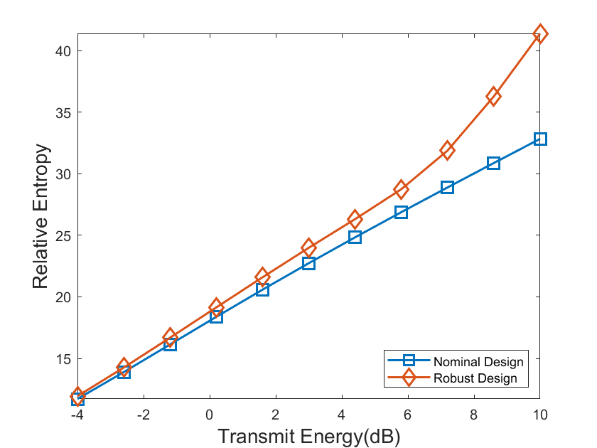
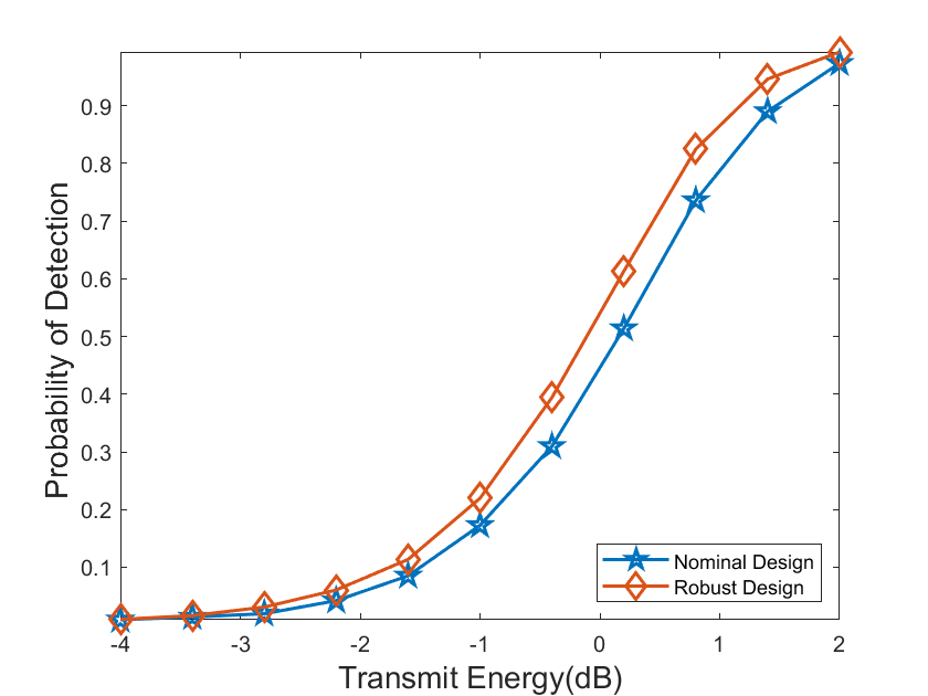
Now we compare the performance of the waveforms synthesized by the proposed algorithm with that of the waveforms synthesized by (5). Note that to design the waveforms by (5), we replace ${\mathbf{H}}$ by the nominal target response matrix ${\mathbf{H}}_{d}$, and ${\textrm{vec}}({\mathbf{H}}_{d})={\mathbf{h}}_{d}$. Fig. 1 shows the relative entropy of the synthesized waveforms versus different transmit energy, where the DOA of the true target is $\theta_{t}=25^{\circ}$ (i.e., a $10^{\circ}$ mismatch between the nominal DOA and the true DOA). We can observe that the waveforms synthesized by the proposed algorithm always have a larger relative entropy. Fig. 2 shows the probabilities of detection associated with Fig. 1, where the NP detector in (8) is used to analyze the detection performance, the probability of false alarm is $P_{fa}=10^{-3}$, and $10^{5}$ Monte Carlo trials are conducted to obtain the threshold and the probability of detection, respectively. We can find that the results in Fig. 2 are consistent with Fig. 1, showing the robustness of the proposed waveforms against the angle mismatch.

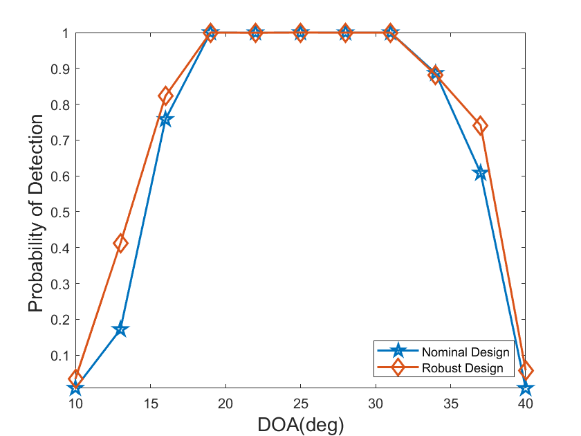
Fig. 3 compares the detection probability of the proposed algorithm with that of the nominal design, where we assume that the true DOA of the target is fixed to be $25^{\circ}$, the nominal DOA of the target varies from $10^{\circ}$ to $40^{\circ}$, and the transmit energy is $P_{t}=1.25$. The results demonstrate that when the angle mismatch is larger than $6^{\circ}$, the proposed algorithm exhibits better robustness.

This paper considered robust waveform design for MIMO radar target detection. A probabilistic model was proposed to describe the target uncertainty, and the relative entropy between the PDF of the observations under two hypotheses was employed as the waveform design metric. To tackle the non-convex waveform design problem, an efficient optimization algorithm based on MM was developed. Numerical results show that the waveforms synthesized by the proposed algorithm are more robust to the target mismatches.

This work was supported in part by the National Natural Science Foundation of China under Grant 62171450 and 61671453, the Anhui Provincial Natural Science Foundation under Grant 2108085J30, and the Young Elite Scientist Sponsorship Program of CAST under Grant 17-JCJQ-QT-041.

References

• [1] J. Li and P. Stoica, MIMO Radar Signal Processing.   Hoboken, NJ, USA: Wiley, 2008.
• [2] A. M. Haimovich, R. S. Blum, and L. J. Cimini, “MIMO radar with widely separated antennas,” IEEE Signal Processing Magazine, vol. 25, no. 1, pp. 116–129, 2008.
• [3] J. Li and P. Stoica, “MIMO radar with colocated antennas,” IEEE Signal Processing Magazine, vol. 24, no. 5, pp. 106–114, 2007.
• [4] H. He, P. Stoica, and J. Li, “Designing unimodular sequence sets with good correlations-including an application to MIMO radar,” IEEE Transactions on Signal Processing, vol. 57, no. 11, pp. 4391–4405, 2009.
• [5] H. He, J. Li, and P. Stoica, Waveform Design for Active Sensing Systems: A Computational Approach.   Cambridge, U.K.: Cambridge Univ. Press, 2012.
• [6] C. Chen and P. P. Vaidyanathan, “MIMO radar waveform optimization with prior information of the extended target and clutter,” IEEE Transactions on Signal Processing, vol. 57, no. 9, pp. 3533–3544, 2009.
• [7] B. Tang and J. Tang, “Joint design of transmit waveforms and receive filters for MIMO radar space-time adaptive processing,” IEEE Transactions on Signal Processing, vol. 64, no. 18, pp. 4707–4722, 2016.
• [8] G. Cui, X. Yu, V. Carotenuto, and L. Kong, “Space-time transmit code and receive filter design for colocated MIMO radar,” IEEE Transactions on Signal Processing, vol. 65, no. 5, pp. 1116–1129, 2017.
• [9] B. Tang, J. Tuck, and P. Stoica, “Polyphase waveform design for MIMO radar space time adaptive processing,” IEEE Transactions on Signal Processing, vol. 68, pp. 2143–2154, 2020.
• [10] A. D. Maio and M. Lops, “Design principles of MIMO radar detectors,” IEEE Transactions on Aerospace and Electronic Systems, vol. 43, no. 3, pp. 886–898, 2007.
• [11] B. Tang, J. Tang, and Y. Peng, “MIMO radar waveform design in colored noise based on information theory,” IEEE Transactions on Signal Processing, vol. 58, no. 9, pp. 4684–4697, 2010.
• [12] B. Tang and J. Li, “Spectrally constrained MIMO radar waveform design based on mutual information,” IEEE Transactions on Signal Processing, vol. 67, no. 3, pp. 821–834, 2019.
• [13] B. Tang, M. M. Naghsh, and J. Tang, “Relative entropy-based waveform design for MIMO radar detection in the presence of clutter and interference,” IEEE Transactions on Signal Processing, vol. 63, no. 14, pp. 3783–3796, 2015.
• [14] B. Tang and P. Stoica, “Information-theoretic waveform design for MIMO radar detection in range-spread clutter,” Signal Processing, vol. 182, p. 107961, 2021.
• [15] B. Tang, J. Tang, and Y. Zhang, “Design of multiple-input-multiple-output radar waveforms for Rician target detection,” IET Radar, Sonar & Navigation, vol. 10, no. 9, pp. 1583–1593, 2016.
• [16] B. Tang, Y. Zhang, and J. Tang, “An efficient minorization maximization approach for MIMO radar waveform optimization via relative entropy,” IEEE Transactions on Signal Processing, vol. 66, no. 2, pp. 400–411, 2018.
• [17] S. M. Kay, Fundamentals of statistical signal processing, vol. ii: detection theory, Prentice-Hall, Upper Saddle River, Newer Jersey, 1998.
• [18] R. A. Horn and C. R. Jonson, Matrix Analysis.   Cambridge, U.K: Cambridge Univ. Press, 1990.
• [19] M. M. Naghsh, M. Modarres-Hashemi, M. A. Kerahroodi, and E. H. M. Alian, “An information theoretic approach to robust constrained code design for MIMO radars,” IEEE Transactions on Signal Processing, vol. 65, no. 14, pp. 3647–3661, 2017.
• [20] S. Boyd and L. Vandenberghe, Convex Optimization.   Cambridge, U.K: Combridge Univ. Press, 2004.
• [21] A. Hjorungnes and D. Gesbert, “Complex-valued matrix differentiation: Techniques and key results,” IEEE Transactions on Signal Processing, vol. 55, no. 6, pp. 2740–2746, 2007.
• [22] B. Tang, J. Liu, H. Wang, and Y. Hu, “Constrained radar waveform design for range profiling,” IEEE Transactions on Signal Processing, vol. 69, pp. 1924–1937, 2021.
• [23] D. S. Bernstein, Matrix Mathematics: Theory, Facts, and Formulas.   Princeton, NJ, USA: Princeton Univ. Press, 2009.
• [24] A. Ben-Tal and M. Teboulle, “Hidden convexity in some nonconvex quadratically constrained quadratic programming,” Math. Program., vol. 72, no. 1, pp. 52–63, 1996.