This paper was converted on www.awesomepapers.org from LaTeX by an anonymous user.
Want to know more? Visit the Converter page.

A quantum extension of SVM-perf for training nonlinear SVMs in almost linear time

Jonathan Allcock jonallcock@tencent.com Tencent Quantum Laboratory    Chang-Yu Hsieh kimhsieh@tencent.com Tencent Quantum Laboratory
(October 2020)
Abstract

We propose a quantum algorithm for training nonlinear support vector machines (SVM) for feature space learning where classical input data is encoded in the amplitudes of quantum states. Based on the classical SVM-perf algorithm of Joachims [1], our algorithm has a running time which scales linearly in the number of training examples mm (up to polylogarithmic factors) and applies to the standard soft-margin 1\ell_{1}-SVM model. In contrast, while classical SVM-perf has demonstrated impressive performance on both linear and nonlinear SVMs, its efficiency is guaranteed only in certain cases: it achieves linear mm scaling only for linear SVMs, where classification is performed in the original input data space, or for the special cases of low-rank or shift-invariant kernels. Similarly, previously proposed quantum algorithms either have super-linear scaling in mm, or else apply to different SVM models such as the hard-margin or least squares 2\ell_{2}-SVM which lack certain desirable properties of the soft-margin 1\ell_{1}-SVM model. We classically simulate our algorithm and give evidence that it can perform well in practice, and not only for asymptotically large data sets.

1 Introduction

Support vector machines (SVMs) are powerful supervised learning models which perform classification by identifying a decision surface which separates data according to their labels [2, 3]. While classifiers based on deep neural networks have increased in popularity in recent years, SVM-based classifiers maintain a number of advantages which make them an appealing choice in certain situations. SVMs are simple models with a smaller number of trainable parameters than neural networks, and thus can be less prone to overfitting and easier to interpret. Furthermore, neural network training may often get stuck in local minima, whereas SVM training is guaranteed to find a global optimum [4]. For problems such as text classification which involve high dimensional but sparse data, linear SVMs — which seek a separating hyperplane in the same space as the input data — have been shown to perform extremely well, and training algorithms exist which scale efficiently, i.e. linearly in [5, 6, 7], or even independent of [8], the number of training examples mm.

In more complex cases, where a nonlinear decision surface is required to classify the data successfully, nonlinear SVMs can be used, which seek a separating hyperplane in a higher dimensional feature space. Such feature space learning typically makes use of the kernel trick [9], a method enabling inner product computations in high or even infinite dimensional spaces to be performed implicitly, without requiring the explicit and resource intensive computation of the feature vectors themselves.

While powerful, the kernel trick comes at a cost: many classical algorithms based on this method scale poorly with mm. Indeed, storing the full kernel matrix KK in memory itself requires O(m2)O(m^{2}) resources, making subquadratic training times impossible by brute-force computation of KK. When KK admits a low-rank approximation though, sampling-based approaches such as the Nystrom method [10] or incomplete Cholesky factorization [11] can be used to obtain O(m)O(m) running times, although it may not be clear a priori whether such a low-rank approximation is possible. Another special case corresponds to so-called shift-invariant kernels [12], which include the popular Gaussian radial basis function (RBF) kernel, where classical sampling techniques can be used to map the high dimensional data into a random low dimensional feature space, which can then be trained by fast linear methods. This method has empirically competed favorably with more sophisticated kernel machines in terms of classification accuracy, at a fraction of the training time. While such a method seems to strike a balance between linear and nonlinear approaches, it cannot be applied to more general kernels. In practice, advanced solvers employ multiple heuristics to improve their performance, which makes rigorous analyses of their performance difficult. However, methods like SVM-Light [13], SMO [14], LIBSVM [15] and SVMTorch [16] still empirically scale approximately quadratically with mm for nonlinear SVMs.

The state-of-the-art in terms of provable computational complexity is the Pegasos algorithm [8]. Based on stochastic sub-gradient descent, Pegasos has constant running time for linear SVMs. For nonlinear SVMs, Pegasos has O(m)O(m) running time, and is not restricted to low-rank or shift-invariant kernels. However, while experiments show that Pegasos does indeed display outstanding performance for linear SVMs, for nonlinear SVMs it is outperformed by other benchmark methods on a number of datasets. On the other hand, the SVM-perf algorithm of Joachims [1] has been shown to outperform similar benchmarks [17], although it does have a number of theoretical drawbacks compared with Pegasos. SVM-perf has O(m)O(m) scaling for linear SVMs, but an efficiency for nonlinear SVMs which either depends on heuristics, or on the presence of a low-rank or shift-invariant kernel, where linear in mm scaling can also be achieved. However, given the strong empirical performance of SVM-perf, it serves as a strong starting point for further improvements, with the aim of overcoming the restrictions in its application to nonlinear SVMs.

Can quantum computers implement SVMs more effectively than classical computers? Rebentrost and Lloyd were the first to consider this question [18], and since then numerous other proposals have been put forward [19, 20, 21, 22, 23]. While the details vary, at a high level these quantum algorithms aim to bring benefits in two main areas: i) faster training and evaluation time of SVMs or ii) greater representational power by encoding the high dimensional feature vectors in the amplitudes of quantum states. Such quantum feature maps enable high dimensional inner products to be computed directly and, by sidestepping the kernel trick, allow classically intractable kernels to be computed. These proposals are certainly intriguing, and open up new possibilities for supervised learning. However, the proposals to date with improved running time dependence on mm for nonlinear SVMs do not apply to the standard soft-margin 1\ell_{1}-SVM model, but rather to variations such as least squares 2\ell_{2}-SVMs[18] or hard-margin SVMs [23]. While these other models are useful in certain scenarios, soft-margin 1\ell_{1}-SVMs have two properties - sparsity of weights and robustness to noise - that make them preferable in many circumstances.

In this work we present a method to extend SVM-perf to train nonlinear soft-margin 1\ell_{1}-SVMs with quantum feature maps in a time that scales linearly (up to polylogarithmic factors) in the number of training examples, and which is not restricted to low-rank or shift-invariant kernels. Provided that one has quantum access to the classical data, i.e. quantum random access memory (qRAM) [24, 25], quantum states corresponding to sums of feature vectors can be efficiently created, and then standard methods employed to approximate the inner products between such quantum states. As the output of the quantum procedure is only an approximation to a desired positive semi-definite (p.s.d.) matrix, it is not itself guaranteed to be p.s.d., and hence an additional classical projection step must be carried out to map on to the p.s.d. cone at each iteration.

Before stating our result in more detail, let us make one remark. It has recently been shown by Tang [26] that the data-structure required for efficient qRAM-based inner product estimation would also enable such inner products to be estimated classically, with only a polynomial slow-down relative to quantum, and her method has been employed to de-quantize a number of quantum machine learning algorithms [26, 27, 28] based on such data-structures. However, in practice, polynomial factors can make a difference, and an analysis of a number of such quantum-inspired classical algorithms [29] concludes that care is needed when assessing their performance relative to the quantum algorithms from which they were inspired. More importantly, in this current work, the quantum states produced using qRAM access are subsequently mapped onto a larger Hilbert space before their inner products are evaluated. This means that the procedure cannot be de-quantized in the same way.

2 Background and Results

Let S={(𝐱1,y1),(𝐱m,ym)}S=\{(\mathbf{x}_{1},y_{1}),\ldots(\mathbf{x}_{m},y_{m})\} be a data set with 𝐱id\mathbf{x}_{i}\in\mathbb{R}^{d}, and labels yi{+1,1}y_{i}\in\{+1,-1\}. Let Φ:d\Phi:\mathbb{R}^{d}\rightarrow\mathcal{H} be a feature map where \mathcal{H} is a real Hilbert space (of finite or infinite dimension) with inner product ,\left\langle\cdot\,,\cdot\right\rangle, and let K:d×dK:\mathbb{R}^{d}\times\mathbb{R}^{d}\rightarrow\mathbb{R} be the associated kernel function defined by K(𝐱,𝐲)=𝖽𝖾𝖿Φ(𝐱),Φ(𝐲)K(\mathbf{x},\mathbf{y})\stackrel{{\scriptstyle\mathsf{def}}}{{=}}\langle\Phi(\mathbf{x}),\Phi(\mathbf{y})\rangle. Let R=maxiΦ(𝐱i)R=\max_{i}\left\|\Phi(\mathbf{x}_{i})\right\| denote the largest 2\ell_{2} norm of the feature mapped vectors. In what follows, \left\|\cdot\right\| will always refer to the 2\ell_{2} norm, and other norms will be explicitly differentiated.

2.1 Support Vector Machine Training

Training a soft-margin 1\ell_{1}-SVM with parameter C>0C>0 corresponds to solving the following optimization problem:

OP 1.

(SVM Primal)

min𝐰,ξi0\displaystyle\quad\underset{\mathbf{w}\in\mathcal{H},\ \xi_{i}\geq 0}{\min} 12𝐰,𝐰+Cmi=1mξi\displaystyle\quad\frac{1}{2}\left\langle\mathbf{w},\mathbf{w}\right\rangle+\frac{C}{m}\sum_{i=1}^{m}\xi_{i}
s.t.\displaystyle s.t. yi𝐰,Φ(xi)1ξii=1,,m\displaystyle\quad y_{i}\left\langle\mathbf{w},\Phi(x_{i})\right\rangle\geq 1-\xi_{i}\quad\forall i=1,\ldots,m

Note that, following [1], we divide iξi\sum_{i}\xi_{i} by mm to capture how CC scales with the training set size. The trivial case Φ(𝐱)=𝐱\Phi(\mathbf{x})=\mathbf{x} corresponds to a linear SVM, i.e. a separating hyperplane is sought in the original input space. When one considers feature maps Φ(𝐱)\Phi(\mathbf{x}) in a high dimensional space, it is more practical to consider the dual optimization problem, which is expressed in terms of inner products, and hence the kernel trick can be employed.

OP 2.

(SVM Dual)

max𝛼\displaystyle\underset{\mathbf{\alpha}}{\max} 12i,j=1myiαiyjαjK(𝐱i,𝐱j)+i=1mαi\displaystyle\quad-\frac{1}{2}\sum_{i,j=1}^{m}y_{i}\alpha_{i}y_{j}\alpha_{j}K(\mathbf{x}_{i},\mathbf{x}_{j})+\sum_{i=1}^{m}\alpha_{i}
s.t. 0αiCmi=1,,m\displaystyle\quad 0\leq\alpha_{i}\leq\frac{C}{m}\qquad\forall i=1,\ldots,m

This is a convex quadratic program with box constraints, for which many classical solvers are available, and which requires time polynomial in mm to solve. For instance, using the barrier method [30] a solution can be found to within εb\varepsilon_{b} in time O(m4log(m/εb))O(m^{4}\log(m/\varepsilon_{b})). Indeed, even the computation of the kernel matrix KK takes time Θ(m2)\Theta(m^{2}), so obtaining subquadratic training times via direct evaluation of KK is not possible.

2.2 Structural SVMs

Joachims [1] showed that an efficient approximation algorithm - with running time O(m)O(m) - for linear SVMs could be obtained by considering a slightly different but related model known as a structural SVM [31], which makes use of linear combinations of label-weighted feature vectors:

Definition 1.

For a given data set S={(𝐱1,y1),,(𝐱m,ym)}S=\left\{(\mathbf{x}_{1},y_{1}),\ldots,(\mathbf{x}_{m},y_{m})\right\}, feature map Φ\Phi, and 𝐜{0,1}m\mathbf{c}\in\{0,1\}^{m}, define

Ψ𝐜=𝖽𝖾𝖿1mi=1mciyiΦ(𝐱i)\displaystyle\Psi_{\mathbf{c}}\stackrel{{\scriptstyle\mathsf{def}}}{{=}}\frac{1}{m}\sum_{i=1}^{m}c_{i}y_{i}\Phi(\mathbf{x}_{i})

With this notation, the structural SVM primal and dual optimization problems are:

OP 3.

(Structural SVM Primal)

min𝐰,ξ0\displaystyle\underset{\mathbf{w}\in\mathcal{H},\ \xi\geq 0}{\min} P(𝐰,ξ)=𝖽𝖾𝖿12𝐰,𝐰+Cξ\displaystyle\quad P(\mathbf{w},\xi)\stackrel{{\scriptstyle\mathsf{def}}}{{=}}\frac{1}{2}\left\langle\mathbf{w},\mathbf{w}\right\rangle+C\xi
s.t. 1mi=1mci𝐰,Ψ𝐜ξ,𝐜{0,1}m\displaystyle\quad\frac{1}{m}\sum_{i=1}^{m}c_{i}-\left\langle\mathbf{w},\Psi_{\mathbf{c}}\right\rangle\leq\xi,\qquad\forall\mathbf{c}\in\{0,1\}^{m}
OP 4.

(Structural SVM Dual)

maxα0\displaystyle\underset{\alpha\geq 0}{\max} D(α)=𝖽𝖾𝖿12𝐜,𝐜{0,1}mα𝐜α𝐜J𝐜𝐜+𝐜{0,1}m𝐜1mα𝐜\displaystyle\,\,D(\alpha)\stackrel{{\scriptstyle\mathsf{def}}}{{=}}-\frac{1}{2}\sum_{\mathbf{c},\mathbf{c}^{\prime}\in\{0,1\}^{m}}\alpha_{\mathbf{c}}\alpha_{\mathbf{c}^{\prime}}J_{\mathbf{c}\mathbf{c}^{\prime}}+\sum_{\mathbf{c}\in\{0,1\}^{m}}\frac{\left\|\mathbf{c}\right\|_{1}}{m}\alpha_{\mathbf{c}}
s.t. 𝐜{0,1}mα𝐜C\displaystyle\sum_{\mathbf{c}\in\{0,1\}^{m}}\alpha_{\mathbf{c}}\leq C

where J𝐜𝐜=Ψ𝐜,Ψ𝐜J_{\mathbf{c}\mathbf{c}^{\prime}}=\left\langle\Psi_{\mathbf{c}},\Psi_{\mathbf{c}^{\prime}}\right\rangle and 1\left\|\cdot\right\|_{1} denotes the 1\ell_{1}-norm.

Whereas the original SVM problem OP 1 is defined by mm constraints and mm slack variables ξi\xi_{i}, the structural SVM OP 3 has only one slack variable ξ\xi but 2m2^{m} constraints, corresponding to each possible binary vector 𝐜{0,1}m\mathbf{c}\in\{0,1\}^{m}. In spite of these differences, the solutions to the two problems are equivalent in the following sense.

Theorem 1 (Joachims [1]).

Let (𝐰,ξ1,,ξm)(\mathbf{w}^{*},\xi^{*}_{1},\ldots,\xi^{*}_{m}) be an optimal solution of OP 1, and let ξ=1mi=1mξi\xi^{*}=\frac{1}{m}\sum_{i=1}^{m}\xi^{*}_{i}. Then (𝐰,ξ)(\mathbf{w}^{*},\xi^{*}) is an optimal solution of OP 3 with the same objective function value. Conversely, for any optimal solution (𝐰,ξ)(\mathbf{w}^{*},\xi^{*}) of OP 3, there is an optimal solution (𝐰,ξ1,,ξm)(\mathbf{w}^{*},\xi^{*}_{1},\ldots,\xi^{*}_{m}) of OP 1 satisfying ξ=1mi=1mξi\xi^{*}=\frac{1}{m}\sum_{i=1}^{m}\xi_{i}, with the same objective function value.

While elegant, Joachims’ algorithm can achieve O(m)O(m) scaling only for linear SVMs — as it requires explicitly computing a set of vectors {Ψ𝐜}\{\Psi_{\mathbf{c}}\} and their inner products — or to shift-invariant or low-rank kernels where sampling methods can be employed. For high dimensional feature maps Φ\Phi not corresponding to shift invariant kernels, computing Ψ𝐜\Psi_{\mathbf{c}} classically is inefficient. We propose instead to embed the feature mapped vectors Φ(𝐱)\Phi(\mathbf{x}) and linear combinations Ψ𝐜\Psi_{\mathbf{c}} in the amplitudes of quantum states, and compute the required inner products efficiently using a quantum computer.

2.3 Our Results

In Section 3 we will formally introduce the concept of a quantum feature map. For now it is sufficient to view this as a quantum circuit which, in time TΦT_{\Phi}, realizes a feature map Φ:d\Phi:\mathbb{R}^{d}\rightarrow\mathcal{H}, with maximum norm max𝐱Φ(𝐱)=R\max_{\mathbf{x}}\left\|\Phi(\mathbf{x})\right\|=R, by mapping the classical data into the state of a multi-qubit system.

Our first main result is a quantum algorithm with running time linear in mm that generates an approximately optimal solution for the structural SVM problem. By Theorem 1, this is equivalent to solving the original soft-margin 1\ell_{1}-SVM.

Quantum nonlinear SVM training: [See Theorems 6 and 7] There is a quantum algorithm that, with probability at least 1δ1-\delta, outputs α^\hat{\alpha} and ξ^\hat{\xi} such that if (𝐰,ξ)(\mathbf{w}^{*},\xi^{*}) is the optimal solution of OP 3, then

P(𝐰^,ξ^)P(𝐰,ξ)min{Cϵ2,ϵ28R2}\displaystyle P(\hat{\mathbf{w}},\hat{\xi})-P(\mathbf{w}^{*},\xi^{*})\leq\min\left\{\frac{C\epsilon}{2},\frac{\epsilon^{2}}{8R^{2}}\right\}

where 𝐰^=𝖽𝖾𝖿𝐜α^𝐜Ψ𝐜\hat{\mathbf{w}}\stackrel{{\scriptstyle\mathsf{def}}}{{=}}\sum_{\mathbf{c}}\hat{\alpha}_{\mathbf{c}}\Psi_{\mathbf{c}}, and (𝐰^,ξ^+3ϵ)(\hat{\mathbf{w}},\hat{\xi}+3\epsilon) is feasible for OP 3. The running time is

O~(CR3log(1/δ)Ψmin(tmax2ϵm+tmax5)TΦ)\displaystyle\tilde{O}\left(\frac{CR^{3}\log(1/\delta)}{\Psi_{\min}}\left(\frac{t^{2}_{\max}}{\epsilon}\cdot m+t_{\max}^{5}\right)T_{\Phi}\right)

where tmax=max{4ϵ,16CR2ϵ2}t_{\max}=\max\left\{\frac{4}{\epsilon},\frac{16CR^{2}}{\epsilon^{2}}\right\}, TΦT_{\Phi} is the time required to compute feature map Φ\Phi on a quantum computer and Ψmin\Psi_{\min} is a term that depends on both the data as well as the choice of quantum feature map.

Here and in what follows, the tilde big-O notation hides polylogarithmic terms. In the Simulation section we show that, in practice, the running time of the algorithm can be significantly faster than the theoretical upper-bound. The solution α^\hat{\alpha} is a tmaxt_{\max}-sparse vector of total dimension 2m2^{m}. Once it has been found, a new data point 𝐱\mathbf{x} can be classified according to

ypred\displaystyle y_{pred} =sgn𝐜α^𝐜Ψ𝐜,Φ(𝐱)\displaystyle=\operatorname{sgn}\left\langle\sum_{\mathbf{c}}\hat{\alpha}_{\mathbf{c}}\Psi_{\mathbf{c}},\Phi(\mathbf{x})\right\rangle
=sgn(𝐜α^𝐜i=1mciyimΦ(𝐱i),Φ(𝐱))\displaystyle=\operatorname{sgn}\left(\sum_{\mathbf{c}}\hat{\alpha}_{\mathbf{c}}\sum_{i=1}^{m}\frac{c_{i}y_{i}}{m}\left\langle\Phi(\mathbf{x}_{i}),\Phi(\mathbf{x})\right\rangle\right)

where ypredy_{pred} is the predicted label of 𝐱\mathbf{x}. This is a sum of O(mtmax)O(mt_{\max}) inner products in feature space, which classical methods require time O(mtmax)O(mt_{\max}) to evaluate in general. Our second result is a quantum algorithm for carrying out this classification with running time independent of mm.

Quantum nonlinear SVM classification: [See Theorem 8] There is a quantum algorithm which, in time

O~(CR3log(1/δ)ΨmintmaxϵTΦ)\displaystyle\tilde{O}\left(\frac{CR^{3}\log(1/\delta)}{\Psi_{\min}}\frac{t_{\max}}{\epsilon}T_{\Phi}\right)

outputs, with probability at least 1δ1-\delta, an estimate to 𝐜α^𝐜Ψ𝐜,Φ(𝐱)\left\langle\sum_{\mathbf{c}}\hat{\alpha}_{\mathbf{c}}\Psi_{\mathbf{c}},\Phi(\mathbf{x})\right\rangle to within ϵ\epsilon accuracy. The sign of the output is then taken as the predicted label.

3 Methods

Our results are based on three main components: Joachims’ linear time classical algorithm SVM-perf, quantum feature maps, and efficient quantum methods for estimating inner products of linear combinations of high dimensional vectors.

3.1 SVM-perf: a linear time algorithm for linear SVMs

On the surface, the structural SVM problems OP 3 and OP 4 look more complicated to solve than the original SVM problems OP 1 and OP 2. However, it turns out that the solution α\alpha^{*} to OP 4 is highly sparse and, consequently, the structural SVM admits an efficient algorithm. Joachims’ original procedure is presented in Algorithm 1.

List of Algorithms 1 SVM-perf [1]: Training structural SVMs via OP 3
  Input: Training set S={(𝐱1,y1),,(𝐱m,ym)}S=\left\{(\mathbf{x}_{1},y_{1}),\ldots,(\mathbf{x}_{m},y_{m})\right\}, SVM hyperparameter C>0C>0, tolerance ϵ>0\epsilon>0, 𝐜{0,1}m\mathbf{c}\in\{0,1\}^{m}.
  
  𝒲{𝐜}\mathcal{W}\leftarrow\{\mathbf{c}\}
  repeat
     (𝐰,ξ)argmin𝐰,ξ012𝐰,𝐰+Cξ(\mathbf{w},\xi)\leftarrow\arg\min_{\mathbf{w},\xi\geq 0}\frac{1}{2}\left\langle\mathbf{w},\mathbf{w}\right\rangle+C\xi
     s.t.𝐜𝒲:1mi=1mci𝐰,Ψ𝐜ξ\quad\quad\quad\text{s.t.}\quad\forall\mathbf{c}\in\mathcal{W}:\quad\frac{1}{m}\sum_{i=1}^{m}c_{i}-\left\langle\mathbf{w},\Psi_{\mathbf{c}}\right\rangle\leq\xi
     for i=1,,mi=1,\ldots,m do
        ci{1yi(𝐰T𝐱i)<10otherwisec^{*}_{i}\leftarrow\begin{cases}1&y_{i}\left(\mathbf{w}^{T}\mathbf{x}_{i}\right)<1\\ 0&\text{otherwise}\end{cases}
     end for
     𝒲𝒲{𝐜}\mathcal{W}\leftarrow\mathcal{W}\cup\{\mathbf{c}^{*}\}
  until  1mi=1mciα𝐜𝒲Ψ𝐜,Ψ𝐜ξ+ϵ\frac{1}{m}\sum_{i=1}^{m}c^{*}_{i}-\sum\alpha_{\mathbf{c}^{\prime}\in\mathcal{W}}\left\langle\Psi_{\mathbf{c}^{\prime}},\Psi_{\mathbf{c}^{*}}\right\rangle\leq\xi+\epsilon
  
  Output: (𝐰,ξ)(\mathbf{w},\xi)

The main idea behind Algorithm 1 is to iteratively solve successively more constrained versions of problem OP 3. That is, a working set of indices 𝒲{0,1}m\mathcal{W}\subseteq\{0,1\}^{m} is maintained such that, at each iteration, the solution (𝐰,ξ)(\mathbf{w},\xi) is only required to satisfy the constraints 1mi=1mci𝐰,Ψcξ\frac{1}{m}\sum_{i=1}^{m}c_{i}-\left\langle\mathbf{w},\Psi_{c}\right\rangle\leq\xi for 𝐜𝒲\mathbf{c}\in\mathcal{W}. The inner for loop then finds a new index 𝐜\mathbf{c}^{*} which corresponds to the maximally violated constraint in OP 3, and this index is added to the working set. The algorithm proceeds until no constraint is violated by more than ϵ\epsilon. It can be shown that each iteration must improve the value of the dual objective by a constant amount, from which it follows that the algorithm terminates in a number of rounds independent of mm.

Theorem 2 (Joachims [1]).

Algorithm 1 terminates after at most max{2ϵ,8CR2ϵ2}\max\left\{\frac{2}{\epsilon},\frac{8CR^{2}}{\epsilon^{2}}\right\} iterations, where R=𝖽𝖾𝖿maxi𝐱iR\stackrel{{\scriptstyle\mathsf{def}}}{{=}}\max_{i}\left\|\mathbf{x}_{i}\right\| is the largest 2\ell_{2}-norm of the training set vectors. For any training set SS and any ϵ>0\epsilon>0, if (𝐰,ξ)(\mathbf{w}^{*},\xi^{*}) is an optimal solution of OP 3, then Algorithm 1 returns a point (𝐰,ξ)(\mathbf{w},\xi) that has a better objective value than (𝐰,ξ)(\mathbf{w}^{*},\xi), and for which (𝐰,ξ+ϵ)(\mathbf{w},\xi+\epsilon) is feasible in OP 3.

In terms of time cost, each iteration tt of the algorithm involves solving the restricted optimization problem

(𝐰,ξ)\displaystyle(\mathbf{w},\xi) =argmin𝐰,ξ012𝐰,𝐰+Cξ\displaystyle=\arg\min_{\mathbf{w},\xi\geq 0}\frac{1}{2}\left\langle\mathbf{w},\mathbf{w}\right\rangle+C\xi
s.t. 𝐜𝒲:1mi=1mci𝐰,Ψcξ\displaystyle\quad\forall\mathbf{c}\in\mathcal{W}:\quad\frac{1}{m}\sum_{i=1}^{m}c_{i}-\left\langle\mathbf{w},\Psi_{c}\right\rangle\leq\xi

which is done in practice by solving the corresponding dual problem, i.e. the same as OP 4 but with summations over 𝐜𝒲\mathbf{c}\in\mathcal{W} instead of over all 𝐜{0,1}\mathbf{c}\in\{0,1\}. This involves computing

  • O(t2)O(t^{2}) matrix elements J𝐜𝐜=Ψ𝐜,Ψ𝐜J_{\mathbf{c}\mathbf{c}^{\prime}}=\left\langle\Psi_{\mathbf{c}},\Psi_{\mathbf{c}^{\prime}}\right\rangle

  • mm inner products 𝐰,𝐱i=𝐜α𝐜Ψ𝐜,𝐱i\left\langle\mathbf{w},\mathbf{x}_{i}\right\rangle=\left\langle\sum_{\mathbf{c}}\alpha_{\mathbf{c}}\Psi_{\mathbf{c}},\mathbf{x}_{i}\right\rangle

where α𝐜\alpha_{\mathbf{c}} is the solution to the dual of the optimization problem in the body of Algorithm 1. In the case of linear SVMs, Ψ𝐜=1mi=1mciyi𝐱i\Psi_{\mathbf{c}}=\frac{1}{m}\sum_{i=1}^{m}c_{i}y_{i}\mathbf{x}_{i} and Ψ𝐜,Ψ𝐜\left\langle\Psi_{\mathbf{c}},\Psi_{\mathbf{c}^{\prime}}\right\rangle can each be explicitly computed in time O(m)O(m). The cost of computing matrix JJ is O(mt2)O(mt^{2}), and subsequently solving the dual takes time polynomial in tt. As Joachims showed that tmax{2ϵ,8Cmaxi𝐱i2ϵ2}t\leq\max\left\{\frac{2}{\epsilon},\frac{8C\max_{i}\left\|\mathbf{x}_{i}\right\|^{2}}{\epsilon^{2}}\right\}, and since 𝐰,𝐱i\left\langle\mathbf{w},\mathbf{x}_{i}\right\rangle can be computed in time O(d)O(d), the entire algorithm therefore has running time linear in mm. Note that Joachims considered the special case of ss-sparse data vectors, for which 𝐰,𝐱i\left\langle\mathbf{w},\mathbf{x}_{i}\right\rangle can be computed in time O(s)O(s) rather than O(d)O(d). In what follows we will not consider any sparsity restrictions.

For nonlinear SVMs, the feature maps Φ(𝐱i)\Phi(\mathbf{x}_{i}) may be of very large dimension, which precludes explicitly computing Ψ𝐜=1mi=1mciyiΦ(𝐱i)\Psi_{\mathbf{c}}=\frac{1}{m}\sum_{i=1}^{m}c_{i}y_{i}\Phi(\mathbf{x}_{i}) and directly evaluating Ψ𝐜,Ψ𝐜\left\langle\Psi_{\mathbf{c}},\Psi_{\mathbf{c}^{\prime}}\right\rangle as is done in SVM-perf. Instead, one must compute J𝐜𝐜=Ψ𝐜,Ψ𝐜=1m2i,j=1mcicjyiyjΦ(𝐱i),Φ(𝐱j)J_{\mathbf{c}\mathbf{c}^{\prime}}=\left\langle\Psi_{\mathbf{c}},\Psi_{\mathbf{c}^{\prime}}\right\rangle=\frac{1}{m^{2}}\sum_{i,j=1}^{m}c_{i}c_{j}y_{i}y_{j}\left\langle\Phi(\mathbf{x}_{i}),\Phi(\mathbf{x}_{j})\right\rangle as a sum of O(m2)O(m^{2}) inner products Φ(𝐱i),Φ(𝐱j)\left\langle\Phi(\mathbf{x}_{i}),\Phi(\mathbf{x}_{j})\right\rangle, which are then each evaluated using the kernel trick. This rules out the possibility of an O(m)O(m) algorithm, at least using methods that rely on the kernel trick to evaluate each Φ(𝐱i),Φ(𝐱j)\left\langle\Phi(\mathbf{x}_{i}),\Phi(\mathbf{x}_{j})\right\rangle. Noting that 𝐰=𝐜α𝐜Ψ𝐜\mathbf{w}=\sum_{\mathbf{c}}\alpha_{\mathbf{c}}\Psi_{\mathbf{c}} , the inner products 𝐰,Φ(𝐱i)\left\langle\mathbf{w},\Phi(\mathbf{x}_{i})\right\rangle are similarly expensive to compute directly classically if the dimension of the feature map is large.

3.2 Quantum feature maps

We now show how quantum computing can be used to efficiently approximate the inner products Ψ𝐜,Ψ𝐜\left\langle\Psi_{\mathbf{c}},\Psi_{\mathbf{c}^{\prime}}\right\rangle and 𝐜α𝐜Ψ𝐜,Φ(𝐱i)\left\langle\sum_{\mathbf{c}}\alpha_{\mathbf{c}}\Psi_{\mathbf{c}},\Phi(\mathbf{x}_{i})\right\rangle, where high dimensional Ψ𝐜\Psi_{\mathbf{c}} can be implemented by a quantum circuit using only a number of qubits logarithmic in the dimension. We first assume that the data vectors 𝐱id\mathbf{x}_{i}\in\mathbb{R}^{d} are encoded in the state of an O(d)O(d)-qubit register |𝐱i\left|\mathbf{x}_{i}\right\rangle via some suitable encoding scheme, e.g. given an integer kk, 𝐱i\mathbf{x}_{i} could be encoded in n=kdn=kd qubits by approximating each of the dd values of 𝐱i\mathbf{x}_{i} by a length kk bit string which is then encoded in a computational basis state of nn qubits. Once encoded, a quantum feature map encodes this information in larger space in the following way:

Definition 2 (Quantum feature map).

Let A=(2)n,B=(2)N\mathcal{H}_{A}=\left(\mathbb{C}^{2}\right)^{\otimes n},\mathcal{H}_{B}=\left(\mathbb{C}^{2}\right)^{\otimes N} be nn-qubit input and NN-qubit output registers respectively . A quantum feature map is a unitary mapping UΦ:ABABU_{\Phi}:\mathcal{H}_{A}\otimes\mathcal{H}_{B}\rightarrow\mathcal{H}_{A}\otimes\mathcal{H}_{B} satisfying

UΦ|𝐱|0=|𝐱|Φ(𝐱),\displaystyle U_{\Phi}\left|\mathbf{x}\right\rangle\left|0\right\rangle=\left|\mathbf{x}\right\rangle\left|\Phi(\mathbf{x})\right\rangle,

for each of the basis states 𝐱{0,1}n\mathbf{x}\in\{0,1\}^{n}, where |Φ(𝐱)=1Φ(𝐱)j=12NΦ(𝐱)j|j\left|\Phi(\mathbf{x})\right\rangle=\frac{1}{\left\|\Phi(\mathbf{x})\right\|}\sum_{j=1}^{2^{N}}\Phi(\mathbf{x})_{j}\left|j\right\rangle, with real amplitudes Φ(𝐱)j\Phi(\mathbf{x})_{j}\in\mathbb{R}. Denote the running time of UΦU_{\Phi} by TΦT_{\Phi}.

Note that the states |Φ(𝐱)\left|\Phi(\mathbf{x})\right\rangle are not necessarily orthogonal. Implementing such a quantum feature map could be done, for instance, through a controlled parameterized quantum circuit.

We also define the quantum state analogy of Ψ𝐜\Psi_{\mathbf{c}} from Definition 1:

Definition 3.

Given a quantum feature map UΦU_{\Phi}, define |Ψ𝐜\left|\Psi_{\mathbf{c}}\right\rangle as

|Ψ𝐜\displaystyle\left|\Psi_{\mathbf{c}}\right\rangle =1Ψ𝐜i=1mciyimΦ(𝐱i)|Φ(𝐱i)\displaystyle=\frac{1}{\left\|\Psi_{\mathbf{c}}\right\|}\sum_{i=1}^{m}\frac{c_{i}y_{i}}{m}\left\|\Phi(\mathbf{x}_{i})\right\|\left|\Phi(\mathbf{x}_{i})\right\rangle

where

Ψ𝐜2=1m2i,j=1mcicjyiyjΦ(𝐱i)Φ(𝐱j)Φ(𝐱i)|Φ(𝐱j)\displaystyle\left\|\Psi_{\mathbf{c}}\right\|^{2}=\frac{1}{m^{2}}\sum_{i,j=1}^{m}c_{i}c_{j}y_{i}y_{j}\left\|\Phi(\mathbf{x}_{i})\right\|\left\|\Phi(\mathbf{x}_{j})\right\|\langle\Phi(\mathbf{x}_{i})|\Phi(\mathbf{x}_{j})\rangle

3.3 Quantum inner product estimation

Let real vectors x,ydx,y\in\mathbb{R}^{d} have corresponding normalized quantum states |x=1xi=1dxi|i\left|x\right\rangle=\frac{1}{\left\|x\right\|}\sum_{i=1}^{d}x_{i}\left|i\right\rangle and |y=1yi=1dyi|i\left|y\right\rangle=\frac{1}{\left\|y\right\|}\sum_{i=1}^{d}y_{i}\left|i\right\rangle. The following result shows how the inner product x,y=x|yxy\left\langle x,y\right\rangle=\langle x|y\rangle\left\|x\right\|\left\|y\right\| can be estimated efficiently on a quantum computer.

Theorem 3 (Robust Inner Product Estimation [32], restated).

Let |x\left|x\right\rangle and |y\left|y\right\rangle be quantum states with real amplitudes and with bounded norms x,yR\left\|x\right\|,\left\|y\right\|\leq R. If |x\left|x\right\rangle and |y\left|y\right\rangle can each be generated by a quantum circuit in time TT, and if estimates of the norms are known to within ϵ/3R\epsilon/3R additive error, then one can perform the mapping |x|y|0|x|y|s\left|x\right\rangle\left|y\right\rangle\left|0\right\rangle\rightarrow\left|x\right\rangle\left|y\right\rangle\left|s\right\rangle where, with probability at least 1δ1-\delta, |sx,y|ϵ\left|s-\langle x,y\rangle\right|\leq\epsilon. The time required to perform this mapping is O~(R2log(1/δ)ϵT)\widetilde{O}\left(\frac{R^{2}\log(1/\delta)}{\epsilon}T\right).

Thus, if one can efficiently create quantum states |Ψ𝐜\left|\Psi_{\mathbf{c}}\right\rangle and estimate the norms Ψ𝐜\left\|\Psi_{\mathbf{c}}\right\|, then the corresponding J𝐜𝐜=Ψ𝐜,Ψ𝐜=Ψ𝐜Ψ𝐜Ψ𝐜|Ψ𝐜J_{\mathbf{c}\mathbf{c}^{\prime}}=\left\langle\Psi_{\mathbf{c}},\Psi_{\mathbf{c}^{\prime}}\right\rangle=\left\|\Psi_{\mathbf{c}}\right\|\left\|\Psi_{\mathbf{c}^{\prime}}\right\|\langle\Psi_{\mathbf{c}}|\Psi_{\mathbf{c}^{\prime}}\rangle can be approximated efficiently. In this section we show that this is possible with a quantum random access memory (qRAM), which is a device that allows classical data to be queried efficiently in superposition. That is, if xdx\in\mathbb{R}^{d} is stored in qRAM, then a query to the qRAM implements the unitary jαj|j|0jαj|j|xj\sum_{j}\alpha_{j}\left|j\right\rangle\left|0\right\rangle\rightarrow\sum_{j}\alpha_{j}\left|j\right\rangle\left|x_{j}\right\rangle. If the elements xjx_{j} of xx arrive as a stream of entries (j,xj)(j,x_{j}) in some arbitrary order, then xx can be stored in a particular data structure [33] in time O~(d)\tilde{O}(d) and, once stored, |x=1xjxj|j\left|x\right\rangle=\frac{1}{\left\|x\right\|}\sum_{j}x_{j}\left|j\right\rangle can be created in time polylogarithmic in dd. Note that when we refer to real-valued data being stored in qRAM, it is implied that the information is stored as a binary representation of the data, so that it may be loaded into a qubit register.

Theorem 4.

Let 𝐜,𝐜{0,1}m\mathbf{c},\mathbf{c}^{\prime}\in\{0,1\}^{m}. If, for all i[m]i\in[m], 𝐱i,ciyimΦ(𝐱i),ciyimΦ(𝐱i)\mathbf{x}_{i},\frac{c_{i}y_{i}}{\sqrt{m}}\left\|\Phi(\mathbf{x}_{i})\right\|,\frac{c^{\prime}_{i}y_{i}}{\sqrt{m}}\left\|\Phi(\mathbf{x}_{i})\right\| are stored in qRAM, and if η𝐜=i=1mciΦ(𝐱i)2m\eta_{\mathbf{c}}=\sqrt{\frac{\sum_{i=1}^{m}c_{i}\left\|\Phi(\mathbf{x}_{i})\right\|^{2}}{m}} and η𝐜=i=1mciΦ(𝐱i)2m\eta_{\mathbf{c}^{\prime}}=\sqrt{\frac{\sum_{i=1}^{m}c^{\prime}_{i}\left\|\Phi(\mathbf{x}_{i})\right\|^{2}}{m}} are known then, with probability at least 1δ1-\delta, an estimate s𝐜𝐜s_{\mathbf{c}\mathbf{c}^{\prime}} satisfying

|s𝐜𝐜Ψ𝐜,Ψ𝐜|\displaystyle\left|s_{\mathbf{c}\mathbf{c}^{\prime}}-\left\langle\Psi_{\mathbf{c}},\Psi_{\mathbf{c}^{\prime}}\right\rangle\right| ϵ\displaystyle\leq\epsilon

can be computed in time

Tcc\displaystyle T_{cc^{\prime}} =O~(log(1/δ)ϵR3min{Ψ𝐜,Ψ𝐜}TΦ)\displaystyle=\tilde{O}\left(\frac{\log(1/\delta)}{\epsilon}\frac{R^{3}}{\min\left\{\left\|\Psi_{\mathbf{c}}\right\|,\left\|\Psi_{\mathbf{c}^{\prime}}\right\|\right\}}T_{\Phi}\right) (1)

where R=maxiΦ(𝐱i)R=\max_{i}\left\|\Phi(\mathbf{x}_{i})\right\|.

A similar result applies to estimating inner products of the form 𝐜αcΨ𝐜,yiΦ(𝐱i)\sum_{\mathbf{c}\alpha_{c}}\left\langle\Psi_{\mathbf{c}},y_{i}\Phi(\mathbf{x}_{i})\right\rangle.

Theorem 5.

Let 𝒲{0,1}m\mathcal{W}\subseteq\{0,1\}^{m} and 𝐜𝒲α𝐜C\sum_{\mathbf{c}\in\mathcal{W}}\alpha_{\mathbf{c}}\leq C. If η𝐜\eta_{\mathbf{c}} are known for all 𝐜𝒲\mathbf{c}\in\mathcal{W} and if 𝐱i\mathbf{x}_{i} and ciyimΦ(𝐱i)\frac{c_{i}y_{i}}{\sqrt{m}}\left\|\Phi(\mathbf{x}_{i})\right\| are stored in qRAM for all i[m]i\in[m] then, with probability at least 1δ1-\delta, 𝐜𝒲α𝐜Ψ𝐜,yiΦ(𝐱i)\sum_{\mathbf{c}\in\mathcal{W}}\alpha_{\mathbf{c}}\left\langle\Psi_{\mathbf{c}},y_{i}\Phi(\mathbf{x}_{i})\right\rangle can be estimated to within error ϵ\epsilon in time

O~(log(1/δ)ϵCR3|𝒲|min𝐜𝒲Ψ𝐜TΦ)\displaystyle\tilde{O}\left(\frac{\log(1/\delta)}{\epsilon}\frac{CR^{3}\left|\mathcal{W}\right|}{\min_{\mathbf{c}\in\mathcal{W}}\left\|\Psi_{\mathbf{c}}\right\|}T_{\Phi}\right)

Proofs of Theorems 4 and 5 are given in Appendix A.

4 Linear Time Algorithm for Nonlinear SVMs

The results of the previous section can be used to generalize Joachims’ algorithm to quantum feature-mapped data. Let Sn+S^{+}_{n} denote the cone of n×nn\times n positive semi-definite matrices. Given Xn×nX\in\mathbb{R}^{n\times n}, let PSn+(X)=argminYSn+YXFP_{S^{+}_{n}}(X)=\arg\min_{Y\in S^{+}_{n}}\left\|Y-X\right\|_{F}, i.e. the projection of XX onto Sn+S^{+}_{n}, where F\left\|\cdot\right\|_{F} is the Frobenius norm. Denote the ii-th row of XX by (X)i\left(X\right)_{i}.

Define IPϵ,δ(x,y)IP_{\epsilon,\delta}(x,y) to be a quantum subroutine which, with probability at least 1δ1-\delta, returns an estimate ss of the inner product of two vectors x,yx,y satisfying |sx,y|ϵ\left|s-\left\langle x,y\right\rangle\right|\leq\epsilon. As we have seen, with appropriate data stored in qRAM, this subroutine can be implemented efficiently on a quantum computer.

Our quantum algorithm for nonlinear structural SVMs is presented in Algorithm 2. At first sight, it appears significantly more complicated than Algorithm 1, but this is due in part to more detailed notation used to aid the analysis later. The key differences are (i) the matrix elements J𝐜𝐜=Ψ𝐜,Ψ𝐜J_{\mathbf{c}\mathbf{c}^{\prime}}=\left\langle\Psi_{\mathbf{c}},\Psi_{\mathbf{c}^{\prime}}\right\rangle are only estimated to precision ϵJ\epsilon_{J} by the quantum subroutine; (ii) as the corresponding matrix JJ is not guaranteed to be positive semi-definite, an additional classical projection step must therefore be carried out to map the estimated matrix on to the p.s.d. cone at each iteration; (iii) In the classical algorithm, the values of cic^{*}_{i} are deduced by ci=max(0,1yi(𝐰T𝐱i))c_{i}^{*}=\max(0,1-y_{i}(\mathbf{w}^{T}\mathbf{x}_{i})) whereas here we can only estimate the inner products 𝐰T,Φ(𝐱i)\left\langle\mathbf{w}^{T},\Phi(\mathbf{x}_{i})\right\rangle to precision ϵ\epsilon, and 𝐰\mathbf{w} is known only implicitly according to 𝐰=𝐜𝒲α𝐜Ψ𝐜\mathbf{w}=\sum_{\mathbf{c}\in\mathcal{W}}\alpha_{\mathbf{c}}\Psi_{\mathbf{c}}. Note that apart from the quantum inner product estimation subroutines, all other computations are performed classically.

List of Algorithms 2 Quantum-classical structural SVM algorithm
  Input: Training set S={(𝐱1,y1),,(𝐱m,ym)}S=\left\{(\mathbf{x}_{1},y_{1}),\ldots,(\mathbf{x}_{m},y_{m})\right\}, SVM hyperparameter CC, quantum feature map UΦU_{\Phi} with maximum norm R=maxiΦ(𝐱i)R=\max_{i}\left\|{\Phi(\mathbf{x}_{i})}\right\|, tolerance parameters ϵ,δ>0\epsilon,\delta>0, 𝐜{0,1}m\mathbf{c}\in\{0,1\}^{m}, tmax1t_{\max}\geq 1.
  
  set t1t\leftarrow 1 and 𝒲1{𝐜}\mathcal{W}_{1}\leftarrow\left\{\mathbf{c}\right\}
  
  for i=1,,mi=1,\ldots,m do
     Store ciyimΦ(𝐱i)\frac{c_{i}y_{i}}{\sqrt{m}}\left\|\Phi(\mathbf{x}_{i})\right\| and 𝐱i\mathbf{x}_{i} in qRAM
  end for
  Compute and store η𝐜=i=1mciΦ(𝐱i)2m\eta_{\mathbf{c}}=\sqrt{\frac{\sum_{i=1}^{m}c_{i}\left\|\Phi(\mathbf{x}_{i})\right\|^{2}}{m}} classically
  
  repeat
     set ϵJ1Cttmax\epsilon_{J}\leftarrow\frac{1}{Ct\,t_{\max}} and δJδ2t2tmax\delta_{J}\leftarrow\frac{\delta}{2t^{2}\,t_{\max}}
     
     for 𝐜,𝐜𝒲t\mathbf{c},\mathbf{c}^{\prime}\in\mathcal{W}_{t} do
        J~𝐜𝐜IPϵJ,δJ(Ψ𝐜,Ψ𝐜)\tilde{J}_{\mathbf{c}\mathbf{c}^{\prime}}\leftarrow IP_{\epsilon_{J},\delta_{J}}(\Psi_{\mathbf{c}},\Psi_{\mathbf{c}^{\prime}})
     end for
     
     J^𝒲tPS|𝒲t|+(J~)\hat{J}_{\mathcal{W}_{t}}\leftarrow P_{S^{+}_{\left|\mathcal{W}_{t}\right|}}(\tilde{J})
     α^(t)argmaxα012𝐜,𝐜𝒲α𝐜α𝐜(J^𝒲t)𝐜𝐜+𝐜𝒲𝐜1mα𝐜\hat{\alpha}^{(t)}\leftarrow\operatorname{argmax}_{\alpha\geq 0}-\frac{1}{2}\sum_{\mathbf{c},\mathbf{c}^{\prime}\in{\mathcal{W}}}\alpha_{\mathbf{c}}\alpha_{\mathbf{c}^{\prime}}\left(\hat{J}_{\mathcal{W}_{t}}\right)_{\mathbf{c}\mathbf{c}^{\prime}}+\sum_{\mathbf{c}\in\mathcal{W}}\frac{\left\|\mathbf{c}\right\|_{1}}{m}\alpha_{\mathbf{c}}
     s.t.𝐜𝒲tα𝐜C\quad\quad\quad\quad\quad\quad\quad\text{s.t.}\quad\sum_{\mathbf{c}\in\mathcal{W}_{t}}\alpha_{\mathbf{c}}\leq C
     Store α^(t)\hat{\alpha}^{(t)} in qRAM
     
     for 𝐜𝒲t\mathbf{c}\in\mathcal{W}_{t} do
        ξ𝐜(t)max{1mi=1mci𝐜𝒲tα^𝐜(t)(J^𝒲t)𝐜𝐜,0}\xi_{\mathbf{c}}^{(t)}\leftarrow\max\left\{\frac{1}{m}\sum_{i=1}^{m}c_{i}-\sum_{\mathbf{c}^{\prime}\in\mathcal{W}_{t}}\hat{\alpha}^{(t)}_{\mathbf{c}^{\prime}}\left(\hat{J}_{\mathcal{W}_{t}}\right)_{\mathbf{c}\mathbf{c}^{\prime}},0\right\}
     end for
     
     set ξ^(t)max𝐜𝒲tξ𝐜(t)+1tmax\hat{\xi}^{(t)}\leftarrow\max_{\mathbf{c}\in\mathcal{W}_{t}}\xi_{\mathbf{c}}^{(t)}+\frac{1}{t_{\max}} and δζδ2mtmax\delta_{\zeta}\leftarrow\frac{\delta}{2m\,t_{\max}}
     
     for i=1,,mi=1,\ldots,m do
        ζiIPϵ,δζ(𝐜𝒲tα^𝐜(t)Ψ𝐜,yiΦ(𝐱i))\zeta_{i}\leftarrow IP_{\epsilon,\delta_{\zeta}}\left(\sum_{\mathbf{c}\in\mathcal{W}_{t}}\hat{\alpha}^{(t)}_{\mathbf{c}}\Psi_{\mathbf{c}},y_{i}\Phi(\mathbf{x}_{i})\right)
        ci(t+1){1ζi<10otherwisec^{(t+1)}_{i}\leftarrow\begin{cases}1&\zeta_{i}<1\\ 0&\text{otherwise}\end{cases}
        Store ci(t+1)yimΦ(𝐱i)\frac{c_{i}^{(t+1)}y_{i}}{\sqrt{m}}\left\|\Phi(\mathbf{x}_{i})\right\| in qRAM
     end for
     
     Compute and store η𝐜(t+1)\eta_{\mathbf{c}^{(t+1)}} classically
     set 𝒲t+1𝒲t{𝐜(t+1)}\mathcal{W}_{t+1}\leftarrow\mathcal{W}_{t}\cup\{\mathbf{c}^{(t+1)}\} and tt+1t\leftarrow t+1
     
  until 1mi=1mmax{0,1ζi}ξ^(t)+2ϵ\frac{1}{m}\sum_{i=1}^{m}\max\left\{0,1-\zeta_{i}\right\}\leq\hat{\xi}^{(t)}+2\epsilon OR t>tmaxt>t_{\max}
  
  Output: α^=α^(t),ξ^=ξ^(t)\hat{\alpha}=\hat{\alpha}^{(t)},\hat{\xi}=\hat{\xi}^{(t)}
Theorem 6.

Let tmaxt_{\max} be a user-defined parameter and let (𝐰,ξ)(\mathbf{w}^{*},\xi^{*}) be an optimal solution of OP 3. If Algorithm 2 terminates in at most tmaxt_{\max} iterations then, with probability at least 1δ1-\delta, it outputs α^\hat{\alpha} and ξ^\hat{\xi} such that 𝐰^=𝐜α^𝐜Ψ𝐜\hat{\mathbf{w}}=\sum_{\mathbf{c}}\hat{\alpha}_{\mathbf{c}}\Psi_{\mathbf{c}} satisfies P(𝐰^,ξ^)P(𝐰,ξ)min{Cϵ2,ϵ28R2}P(\hat{\mathbf{w}},\hat{\xi})-P(\mathbf{w}^{*},\xi^{*})\leq\min\left\{\frac{C\epsilon}{2},\frac{\epsilon^{2}}{8R^{2}}\right\}, and (𝐰^,ξ^+3ϵ)(\hat{\mathbf{w}},\hat{\xi}+3\epsilon) is feasible for OP 3. If tmaxmax{4ϵ,16CR2ϵ2}t_{\max}\geq\max\left\{\frac{4}{\epsilon},\frac{16CR^{2}}{\epsilon^{2}}\right\} then the algorithm is guaranteed to terminate in at most tmaxt_{\max} iterations.

Proof.

See Appendix B. ∎

Theorem 7.

Algorithm 2 has a time complexity of

O~(CR3log(1/δ)Ψmin(tmax2ϵm+tmax5)TΦ)\displaystyle\tilde{O}\left(\frac{CR^{3}\log(1/\delta)}{\Psi_{\min}}\left(\frac{t^{2}_{\max}}{\epsilon}\cdot m+t_{\max}^{5}\right)T_{\Phi}\right) (2)

where Ψmin=min𝐜𝒲tfΨ𝐜\Psi_{\min}=\min_{\mathbf{c}\in\mathcal{W}_{t_{f}}}\left\|\Psi_{\mathbf{c}}\right\|, and tftmaxt_{f}\leq t_{\max} is the iteration at which the algorithm terminates.

Proof.

See Appendix C.

The total number of outer-loop iterations (indexed by tt) of Algorithm 2 is upper-bounded by the choice of tmaxt_{\max}. One may wonder why we do not simply set tmax=max{4ϵ,16CR2ϵ2}t_{\max}=\max\left\{\frac{4}{\epsilon},\frac{16CR^{2}}{\epsilon^{2}}\right\} as this would ensure that, with high probability, the algorithm outputs a nearly optimal solution. The reason is that tmaxt_{\max} also affects the the quantities ϵJ=1Cttmax\epsilon_{J}=\frac{1}{Ctt_{\max}}, δJ=δ2t2tmax\delta_{J}=\frac{\delta}{2t^{2}t_{\max}} and δζ=δ2mtmax\delta_{\zeta}=\frac{\delta}{2mt_{\max}}. These in turn impact the running time of the two quantum inner product estimation subroutines that take place in each iteration, e.g. the first quantum inner product estimation subroutine has running time that scales like log(1/δJ)ϵJ\frac{\log(1/\delta_{J})}{\epsilon_{J}}. While the upper-bound on tmaxt_{\max} of max{4ϵ,16CR2ϵ2}\max\left\{\frac{4}{\epsilon},\frac{16CR^{2}}{\epsilon^{2}}\right\} is independent of mm, it can be large for reasonable values of the other algorithm parameters CC, ϵ\epsilon, δ\delta and RR. For instance, the choice of (C,ϵ,δ,R)=(104,0.01,0.1,1)(C,\epsilon,\delta,R)=(10^{4},0.01,0.1,1) which, as we show in the Simulation section, lead to good classification performance on the datasets we consider, corresponds to tmax=1.6×10⁹t_{\max}=1.6\times 10^{9}, and log(1/δJ)ϵJ1.6×1013\frac{\log(1/\delta_{J})}{\epsilon_{J}}\geq 1.6\times 10^{13}. In practice, we find that this upper-bound on tmaxt_{\max} is very loose, and the situation is far better in practice: the algorithm can terminate successfully in very few iterations with much smaller values of tmaxt_{\max}. In the examples we consider, the algorithm terminates successfully before tt reaches tmax=50t_{\max}=50, corresponding to log(1/δJ)ϵJ3.7×108\frac{\log(1/\delta_{J})}{\epsilon_{J}}\leq 3.7\times 10^{8}.

The running time of Algorithm 2 also depends on the quantity Ψmin\Psi_{\min} which is a function of both the dataset as well as the quantum feature map chosen. While this can make Ψmin\Psi_{\min} hard to predict, we will again see in the Simulation section that in practice the situation is optimistic: we empirically find that Ψmin\Psi_{\min} is neither too small, nor does it scale noticeably with mm or the dimension of the quantum feature map.

4.1 Classification of new test points

As is standard in SVM theory, the solution α^\hat{\alpha} from Algorithm 2 can be used to classify a new data point 𝐱\mathbf{x} according to

ypred=sgn𝐜α^𝐜Ψ𝐜,Φ(𝐱)\displaystyle y_{pred}=\operatorname{sgn}\left\langle\sum_{\mathbf{c}}\hat{\alpha}_{\mathbf{c}}\Psi_{\mathbf{c}},\Phi(\mathbf{x})\right\rangle

where ypredy_{pred} is the predicted label of 𝐱\mathbf{x}. From Theorem 5, and noting that |𝒲|tmax\left|\mathcal{W}\right|\leq t_{\max}, we obtain the following result:

Theorem 8.

Let α^\hat{\alpha} be the output of Algorithm 2, and let 𝐱\mathbf{x} be stored in qRAM. There is a quantum algorithm that, with probability at least 1δ1-\delta, estimates the inner product 𝐜α^𝐜Ψ𝐜,Φ(𝐱)\left\langle\sum_{\mathbf{c}}\hat{\alpha}_{\mathbf{c}}\Psi_{\mathbf{c}},\Phi(\mathbf{x})\right\rangle to within error ϵ\epsilon in time O~(CR3log(1/δ)ΨmintmaxϵTΦ)\tilde{O}\left(\frac{CR^{3}\log(1/\delta)}{\Psi_{\min}}\frac{t_{\max}}{\epsilon}T_{\Phi}\right)

Taking the sign of the output then completes the classification.

5 Simulation

While the true performance of our algorithms for large mm and high dimensional quantum feature maps necessitate a fault-tolerant quantum computer to evaluate, we can gain some insight into how it behaves by performing smaller scale numerical experiments on a classical computer. In this section we empirically find that the algorithm can have good performance in practice, both in terms of classification accuracy as well as in terms of the parameters which impact running time.

5.1 Data set

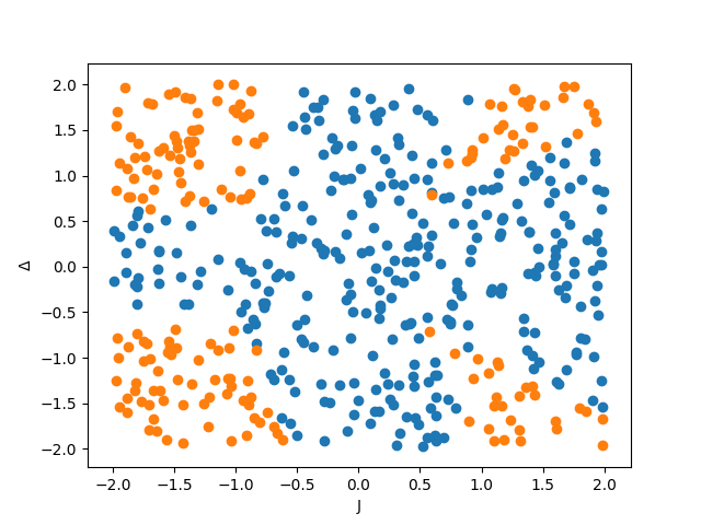
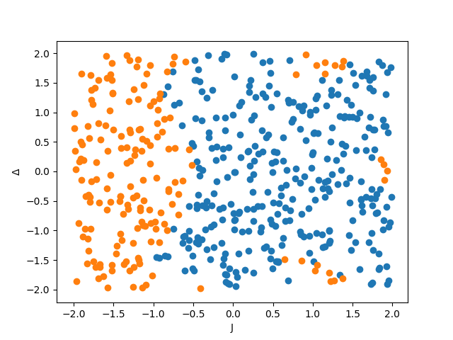
To test our algorithm we need to choose both a data set as well as a quantum feature map. The general question of what constitutes a good quantum feature map, especially for classifying classical data sets, is an open problem and beyond the scope of this investigation. However, if the data is generated from a quantum problem, then physical intuition may guide our choice of feature map. We therefore consider the following toy example which is nonetheless instructive. Let HNH_{N} be the Hamiltonian of a generalized Ising Hamiltonian on NN spins

HN(J,Δ,Γ)\displaystyle H_{N}(\vec{J},\vec{\Delta},\vec{\Gamma}) =j=1NJjZjZj+1+j=1N(ΔjXj+ΓjZj)\displaystyle=-\sum_{j=1}^{N}J_{j}Z_{j}\otimes Z_{j+1}+\sum_{j=1}^{N}\left(\Delta_{j}X_{j}+\Gamma_{j}Z_{j}\right) (3)

where J,Δ,Γ\vec{J},\vec{\Delta},\vec{\Gamma} are vectors of real parameters to be chosen, and Zj,XjZ_{j},X_{j} are Pauli ZZ and XX operators acting on the jj-th qubit in the chain, respectively. We generate a data set by randomly selecting mm points (J,Δ,Γ)(\vec{J},\vec{\Delta},\vec{\Gamma}) and labelling them according to whether the expectation value of the operator M=1N(jZj)2M=\frac{1}{N}\left(\sum_{j}Z_{j}\right)^{2} with respect to the ground state of HN(J,Δ,Γ)H_{N}(\vec{J},\vec{\Delta},\vec{\Gamma}) satisfies

M\displaystyle\langle M\rangle {μ0(+1 labels)<μ0(1 labels)\displaystyle\quad\begin{cases}\geq\mu_{0}&(+1\text{ labels})\\ <\mu_{0}&(-1\text{ labels})\end{cases} (4)

for some cut-off value μ0\mu_{0}, i.e. the points are labelled depending on whether the average total magnetism squared is above or below μ0\mu_{0}. In our simulations we consider a special case of (3) where Jj=JcoskJπ(j1)NJ_{j}=J\cos\frac{k_{J}\pi(j-1)}{N}, Δj=ΔsinkΔπjN\Delta_{j}=\Delta\sin\frac{k_{\Delta}\pi j}{N} and Γj=Γ\Gamma_{j}=\Gamma, where J,kJ,Δ,kΔ,ΓJ,k_{J},\Delta,k_{\Delta},\Gamma are real. Examples of data sets SN,mS_{N,m} corresponding to such a Hamiltonian, whose parameters we notate by

SN,m(μ0,J,kJ,Δ,kΔ,Γ),\displaystyle S_{N,m}(\mu_{0},J,k_{J},\Delta,k_{\Delta},\Gamma),

can be found in Fig 1.

Refer to caption
Refer to caption
Figure 1: Sample data sets (left) S5,500(1.5,J,1,Δ,3,0.5)S_{5,500}(1.5,J,1,\Delta,3,0.5) and (right) S8,500(2.4,J,1,Δ,2,0.5)S_{8,500}(2.4,J,1,\Delta,2,0.5). Blue and orange colors indicated +1+1 and 1-1 labels respectively. In each case 500500 data points (J,Δ)(J,\Delta) were generated uniformly at random in the range [2,2]2[-2,2]^{2}.

5.2 Quantum feature map

For quantum feature map we choose

|Ψ(J,Δ,Γ)\displaystyle\left|\Psi(\vec{J},\vec{\Delta},\vec{\Gamma})\right\rangle =|0|0|0+|1|ψGS|ψGS2\displaystyle=\frac{\left|0\right\rangle\left|0\right\rangle\left|0\right\rangle+\left|1\right\rangle\left|\psi_{GS}\right\rangle\left|\psi_{GS}\right\rangle}{\sqrt{2}} (5)

where |ψGS\left|\psi_{GS}\right\rangle is the ground state of (3) and, as it is a normalized state, has corresponding value of R=1R=1. We compute such feature maps classically by explicitly diagonalizing HNH_{N}. In a real implementation of our algorithm on a quantum computer, such a feature map would be implemented by a controlled unitary for generating the (approximate) ground state of HNH_{N}, which could be done by a variety of methods e.g. by digitized adiabatic evolution or methods based on imaginary time evolution [34, 35], with running time TϕT_{\phi} dependent on the degree of accuracy required. The choice of (5) is motivated by noting that condition (4) is equivalent to determining the sign of W,Ψ\left\langle W,\Psi\right\rangle, where WW is a vector which depends only on μ0\mu_{0}, and not on the choice of parameters in HNH_{N} (see Appendix E). By construction, WW defines a separating hyperplane for the data, so the chosen quantum feature map separate the data in feature space. As the Hamiltonian is real, it has a set of real eigenvectors and hence |Ψ\left|\Psi\right\rangle can be defined to have real amplitudes, as required.

5.3 Numerical results

We first evaluate the performance of our algorithm on data sets SN,mS_{N,m} for N=6N=6 and increasing orders of mm from 10210^{2} to 10510^{5}.

  • For each value of mm, a data set S6,m(μ0,J,kJ,Δ,kΔ,Γ)S_{6,m}(\mu_{0},J,k_{J},\Delta,k_{\Delta},\Gamma) was generated for points (J,Δ)(J,\Delta) sampled uniformly at random in the range [2,2]2[-2,2]^{2}.

  • The values of μ0,kj,kΔ,Γ\mu_{0},k_{j},k_{\Delta},\Gamma were fixed and chosen to give roughly balanced data, i.e. the ratio of +1+1 to 1-1 labels is no more than 70:30 in favor of either label.

  • Each set of mm data points was divided into training and test sets in the ratio 70:30, and training was performed according to Algorithm 2 with parameters (C,ϵ,δ,tmax)=(104,102,101,50)(C,\epsilon,\delta,t_{\max})=(10^{4},10^{-2},10^{-1},50).

  • These values of CC and ϵ\epsilon were selected to give classification accuracy competitive with classical SVM algorithms utilizing standard Gaussian radial basis function (RBF) kernels, with hyperparameters trained using a subset of the training set of size 20%20\% used for hold-out validation. Note that the quantum feature maps do not have any similar tunable parameters, and a modification of (5), for instance to include a tunable weighting between the two parts of the superposition, could be introduced to further improve performance.

  • The quantum IPϵ,δIP_{\epsilon,\delta} inner product estimations in the algorithm were approximated by adding Gaussian random noise to the true inner product, such that the resulting inner product was within ϵ\epsilon of the true value with probability at least 1δ1-\delta. Classically simulating quantum IPϵ,δIP_{\epsilon,\delta} inner product estimation with inner products distributed according to the actual quantum procedures underlying Theorems 4 and 5 was too computationally intensive in general to perform. However, these were tested on small data sets and quantum feature vectors, and found to behave very similarly to adding Gaussian random noise. This is consistent with the results of the numerical simulations in [32].

Note that the values of C,ϵ,δC,\epsilon,\delta chosen correspond to max{4ϵ,16CR2ϵ2}>109\max\left\{\frac{4}{\epsilon},\frac{16CR^{2}}{\epsilon^{2}}\right\}>10^{9}. This is an upper-bound on the number of iterations tmaxt_{\max} needed for the algorithm to converge to a good solution. However, we find empirically that tmax=50t_{\max}=50 is sufficient for the algorithm to terminate with a good solution across the range of mm we consider.

The results are shown in Table 1. We find that (i) with these choices of C,ϵ,δ,tmaxC,\epsilon,\delta,t_{\max} our algorithm has high classification accuracy, competitive with standard classical SVM algorithms utilizing RBF kernels with optimized hyperparameters. (ii) Ψmin\Psi_{\min} is of the order 10210^{-2} in these cases, and does scale noticeably over the range of mm from 10210^{2} to 10510^{5}. If Ψmin\Psi_{\min} were to decrease polynomially (or worse, exponentially) in mm then this would be a severe limitation of our algorithm. Fortunately this does not appear to be the case.

mm 10210^{2} 10310^{3} 10410^{4} 10510^{5}
Ψmin\Psi_{\min} 0.010 0.018 0.016 0.011
iterations 36 38 39 38
accuracy (%)(\%) 93.3 99.3 99.0 98.9
RBF accuracy (%)(\%) 86.7 96.0 99.0 99.7
Table 1: Ψmin\Psi_{\min}, iterations tt until termination, and classification accuracy of Algorithm 2 on data sets with parameters S6,m(1.8,J,1,Δ,9,0.2)S_{6,m}(1.8,J,1,\Delta,9,0.2) for mm randomly chosen points (J,Δ)[2,2]2(J,\Delta)\in[-2,2]^{2}, with mm in the range m=102m=10^{2} to m=105m=10^{5}. Algorithm parameters were chosen to be (C,ϵ,δ,tmax)=(104,102,101,50)(C,\epsilon,\delta,t_{\max})=(10^{4},10^{-2},10^{-1},50). The classification accuracy of classical SVMs with Gaussian radial basis function kernels and optimized hyperparameters is given for comparison.

We further investigate the behaviour of Ψmin\Psi_{\min} by generating data sets SN,mS_{N,m} for fixed m=1000m=1000 and NN ranging from 44 to 88. For each NN, we generate 100100 random data sets SN,m(μ0,J,kJ,Δ,kΔ,Γ)S_{N,m}(\mu_{0},J,k_{J},\Delta,k_{\Delta},\Gamma), where each data set consists of 10001000 points (J,Δ)(J,\Delta) sampled uniformly at random in the range [2,2]2[-2,2]^{2}, and random values of μo,kJ,kΔ,Γ\mu_{o},k_{J},k_{\Delta},\Gamma chosen to give roughly balanced data sets as before. Unlike before, we do not divide the data into training and test sets. Instead, we perform training on the entire data set, and record the value of Ψmin\Psi_{\min} in each instance. The results are given in Table 2 and show that across this range of NN (i) the average value Ψ¯min\bar{\Psi}_{\min} is of order 10210^{-2} (ii) the spread around this average is fairly tight, and the minimum value of Ψmin\Psi_{\min} in any single instance is of order 10310^{-3}. These support the results of the first experiment, and indicate that the value of Ψmin\Psi_{\min} may not adversely affect the running time of the algorithm in practice.

NN 44 5 66 7 88
Ψ¯min(102)\bar{\Psi}_{\min}(10^{-2}) 1.28 1.34 1.32 1.44 1.16
min(Ψmin)\min(\Psi_{\min}) (103)(10^{-3}) 3.41 2.33 3.16 3.82 3.96
s.d. (10310^{-3}) 8.6 20.4 16.2 19.6 6.4
Table 2: Average value, minimum value, and standard deviation of Ψmin\Psi_{\min} for random data sets generated SN,1000(μ0,J,kJ,Δ,kΔ,Γ)S_{N,1000}(\mu_{0},J,k_{J},\Delta,k_{\Delta},\Gamma). For each value of NN, 100 instances (of m=1000m=1000 data points each) were generated for random values of kJ,kΔk_{J},k_{\Delta} and Γ\Gamma, with μ0=3N\mu_{0}=3N . Algorithm 2 was trained using parameters (C,ϵ,δ,tmax)=(104,102,101,50)(C,\epsilon,\delta,t_{\max})=(10^{4},10^{-2},10^{-1},50).

6 Conclusions

We have proposed a quantum extension of SVM-perf for training nonlinear soft-margin 1\ell_{1}-SVMs in time linear in the number of training examples mm, up to polylogarithmic factors, and given numerical evidence that the algorithm can perform well in practice as well as in theory. This goes beyond classical SVM-perf, which achieves linear mm scaling only for linear SVMs or for feature maps corresponding to low-rank or shift-invariant kernels, and brings the theoretical running time and applicability of SVM-perf in line with the classical Pegasos algorithm which — in spite of having best-in-class asymptotic guarantees — has empirically been outperformed by other methods on certain datasets. Our algorithm also goes beyond previous quantum algorithms which achieve linear or better scaling in mm for other variants of SVMs, which lack some of the desirable properties of the soft-margin 1\ell_{1}-SVM model. Following this work, it is straightforward to propose a quantum extension of Pegasos. An interesting question to consider is how such an algorithm would perform against the quantum SVM-perf algorithm we have presented here.

Another important direction for future research is to investigate methods for selecting good quantum feature maps and associated values of RR for a given problem. While work has been done on learning quantum feature maps by training parameterizable quantum circuits [36, 37, 19, 38], a deeper understanding of quantum feature map construction and optimization is needed. In particular, the question of when an explicit quantum feature map can be advantageous compared to the classical kernel trick – as implemented in Pegasos or other state-of-the-art algorithms – needs further investigation. Furthermore, in classical SVM training, typically one of a number of flexible, general purpose kernels such as the Gaussian RBF kernel can be employed in a wide variety of settings. Whether similar, general purpose quantum feature maps can be useful in practice is an open problem, and one that could potentially greatly affect the adoption of quantum algorithms as a useful tool for machine learning.

7 Acknowledgements

We are grateful to Shengyu Zhang for many helpful discussions and feedback on the manuscript.

References

  • Joachims [2006] Thorsten Joachims. Training linear SVMs in linear time. In Proceedings of the 12th ACM SIGKDD international conference on Knowledge discovery and data mining, pages 217–226. ACM, 2006. doi: 10.1145/1150402.1150429.
  • Boser et al. [1992] Bernhard E Boser, Isabelle M Guyon, and Vladimir N Vapnik. A training algorithm for optimal margin classifiers. In Proceedings of the fifth annual workshop on Computational learning theory, pages 144–152. ACM, 1992. doi: 10.1145/130385.130401.
  • Cortes and Vapnik [1995] Corinna Cortes and Vladimir Vapnik. Support-vector networks. Machine Learning, 20(3):273–297, 1995. doi: 10.1023/A:1022627411411.
  • Burges [1998] Christopher JC Burges. A tutorial on support vector machines for pattern recognition. Data mining and knowledge discovery, 2(2):121–167, 1998. doi: 10.1023/A:1009715923555.
  • Ferris and Munson [2002] Michael C Ferris and Todd S Munson. Interior-point methods for massive support vector machines. SIAM Journal on Optimization, 13(3):783–804, 2002. doi: 10.1137/S1052623400374379.
  • Mangasarian and Musicant [2001] Olvi L Mangasarian and David R Musicant. Lagrangian support vector machines. Journal of Machine Learning Research, 1(Mar):161–177, 2001. doi: 10.1162/15324430152748218.
  • Keerthi and DeCoste [2005] S Sathiya Keerthi and Dennis DeCoste. A modified finite Newton method for fast solution of large scale linear SVMs. Journal of Machine Learning Research, 6(Mar):341–361, 2005.
  • Shalev-Shwartz et al. [2011] Shai Shalev-Shwartz, Yoram Singer, Nathan Srebro, and Andrew Cotter. Pegasos: Primal Estimated sub-GrAdient SOlver for SVM. Mathematical programming, 127(1):3–30, 2011. doi: 10.1145/1273496.1273598.
  • Scholkopf and Smola [2001] Bernhard Scholkopf and Alexander J Smola. Learning with kernels: support vector machines, regularization, optimization, and beyond. MIT press, 2001.
  • Williams and Seeger [2001] Christopher KI Williams and Matthias Seeger. Using the Nyström method to speed up kernel machines. In Advances in Neural Information Processing Systems, pages 682–688, 2001.
  • Fine and Scheinberg [2001] Shai Fine and Katya Scheinberg. Efficient SVM training using low-rank kernel representations. Journal of Machine Learning Research, 2(Dec):243–264, 2001.
  • Rahimi and Recht [2008] Ali Rahimi and Benjamin Recht. Random features for large-scale kernel machines. In Advances in Neural Information Processing Systems, pages 1177–1184, 2008.
  • Joachims [1999] Thorsten Joachims. Making large-scale SVM learning practical. In Advances in Kernel Methods-Support Vector Learning. MIT-press, 1999.
  • Platt [1999] John C Platt. Fast training of support vector machines using sequential minimal optimization. MIT press, 1999.
  • Chang and Lin [2011] Chih-Chung Chang and Chih-Jen Lin. LIBSVM: A library for support vector machines. ACM Transactions on Intelligent Systems and Technology, 2(3):27, 2011. doi: 10.1145/1961189.1961199.
  • Collobert and Bengio [2001] Ronan Collobert and Samy Bengio. SVMTorch: Support vector machines for large-scale regression problems. Journal of Machine Learning Research, 1(Feb):143–160, 2001. doi: 10.1162/15324430152733142.
  • Joachims and Yu [2009] Thorsten Joachims and Chun-Nam John Yu. Sparse kernel SVMs via cutting-plane training. Machine Learning, 76(2-3):179–193, 2009. doi: 10.1007/s10994-009-5126-6.
  • Rebentrost et al. [2014] Patrick Rebentrost, Masoud Mohseni, and Seth Lloyd. Quantum support vector machine for big data classification. Physical Review Letters, 113(13):130503, 2014. doi: 10.1103/PhysRevLett.113.130503.
  • Havlíček et al. [2019] Vojtěch Havlíček, Antonio D Córcoles, Kristan Temme, Aram W Harrow, Abhinav Kandala, Jerry M Chow, and Jay M Gambetta. Supervised learning with quantum-enhanced feature spaces. Nature, 567(7747):209–212, 2019. doi: 10.1038/s41586-019-0980-2.
  • Schuld and Killoran [2019] Maria Schuld and Nathan Killoran. Quantum machine learning in feature hilbert spaces. Physical Review Letters, 122(4):040504, 2019. doi: 10.1103/PhysRevLett.122.040504.
  • Kerenidis et al. [2019] Iordanis Kerenidis, Anupam Prakash, and Dániel Szilágyi. Quantum algorithms for second-order cone programming and support vector machines. arXiv preprint arXiv:1908.06720, 2019.
  • Arodz and Saeedi [2019] Tomasz Arodz and Seyran Saeedi. Quantum sparse support vector machines. arXiv preprint arXiv:1902.01879, 2019.
  • Li et al. [2019] Tongyang Li, Shouvanik Chakrabarti, and Xiaodi Wu. Sublinear quantum algorithms for training linear and kernel-based classifiers. In Proceedings of the 36th International Conference on Machine Learning. PMLR, 2019.
  • Giovannetti et al. [2008] Vittorio Giovannetti, Seth Lloyd, and Lorenzo Maccone. Quantum random access memory. Physical Review Letters, 100(16):160501, 2008. doi: 10.1103/PhysRevLett.100.160501.
  • Prakash [2014] Anupam Prakash. Quantum algorithms for linear algebra and machine learning. PhD thesis, UC Berkeley, 2014.
  • Tang [2019] Ewin Tang. A quantum-inspired classical algorithm for recommendation systems. In Proceedings of the 51st Annual ACM SIGACT Symposium on Theory of Computing, pages 217–228, 2019. doi: 10.1145/3313276.3316310.
  • Tang [2018] Ewin Tang. Quantum-inspired classical algorithms for principal component analysis and supervised clustering. arXiv preprint arXiv:1811.00414, 2018.
  • Gilyén et al. [2018] András Gilyén, Seth Lloyd, and Ewin Tang. Quantum-inspired low-rank stochastic regression with logarithmic dependence on the dimension. arXiv preprint arXiv:1811.04909, 2018.
  • Arrazola et al. [2020] Juan Miguel Arrazola, Alain Delgado, Bhaskar Roy Bardhan, and Seth Lloyd. Quantum-inspired algorithms in practice. Quantum, 4:307, 2020. doi: 10.22331/q-2020-08-13-307.
  • Boyd and Vandenberghe [2004] Stephen Boyd and Lieven Vandenberghe. Convex optimization. Cambridge university press, 2004. doi: 10.1017/CBO9780511804441.
  • Tsochantaridis et al. [2005] Ioannis Tsochantaridis, Thorsten Joachims, Thomas Hofmann, and Yasemin Altun. Large margin methods for structured and interdependent output variables. Journal of Machine Learning Research, 6(Sep):1453–1484, 2005.
  • Allcock et al. [2020] Jonathan Allcock, Chang-Yu Hsieh, Iordanis Kerenidis, and Shengyu Zhang. Quantum algorithms for feedforward neural networks. ACM Transactions on Quantum Computing, 1(1), 2020. doi: 10.1145/3411466.
  • Kerenidis and Prakash [2017] Iordanis Kerenidis and Anupam Prakash. Quantum recommendation systems. In 8th Innovations in Theoretical Computer Science Conference (ITCS 2017). Schloss Dagstuhl-Leibniz-Zentrum fuer Informatik, 2017. doi: 10.4230/LIPIcs.ITCS.2017.49.
  • Motta et al. [2020] Mario Motta, Chong Sun, Adrian TK Tan, Matthew J O’Rourke, Erika Ye, Austin J Minnich, Fernando GSL Brandão, and Garnet Kin-Lic Chan. Determining eigenstates and thermal states on a quantum computer using quantum imaginary time evolution. Nature Physics, 16(2):205–210, 2020. doi: 10.1038/s41567-019-0704-4.
  • Hsieh et al. [2019] Chang-Yu Hsieh, Qiming Sun, Shengyu Zhang, and Chee Kong Lee. Unitary-coupled restricted boltzmann machine ansatz for quantum simulations. arxiv prepring quant-ph/1912.02988, 2019.
  • Romero et al. [2017] Jonathan Romero, Jonathan P Olson, and Alan Aspuru-Guzik. Quantum autoencoders for efficient compression of quantum data. Quantum Science and Technology, 2(4):045001, 2017. doi: 10.1088/2058-9565/aa8072.
  • Farhi and Neven [2018] Edward Farhi and Hartmut Neven. Classification with quantum neural networks on near term processors. arXiv preprint arXiv:1802.06002, 2018.
  • Lloyd et al. [2020] Seth Lloyd, Maria Schuld, Aroosa Ijaz, Josh Isaac, and Nathan Killoran. Quantum embeddings for machine learning. arXiv preprint arXiv:2001.03622, 2020.
  • Brassard et al. [2002] Gilles Brassard, Peter Hoyer, Michele Mosca, and Alain Tapp. Quantum amplitude amplification and estimation. Contemporary Mathematics, 305:53–74, 2002.

Appendix A Proofs of Theorem 4 and Theorem 5

Lemma 1.

If 𝐱1,,𝐱md\mathbf{x}_{1},\ldots,\mathbf{x}_{m}\in\mathbb{R}^{d} and c1y1mΦ(𝐱1),,cmymmΦ(𝐱m)\frac{c_{1}y_{1}}{\sqrt{m}}\left\|\Phi(\mathbf{x}_{1})\right\|,\ldots,\frac{c_{m}y_{m}}{\sqrt{m}}\left\|\Phi(\mathbf{x}_{m})\right\| for 𝐜{0,1}m\mathbf{c}\in\{0,1\}^{m} are stored in qRAM, and if η𝐜=i=1mciΦ(𝐱i)2m\eta_{\mathbf{c}}=\sqrt{\frac{\sum_{i=1}^{m}c_{i}\left\|\Phi(\mathbf{x}_{i})\right\|^{2}}{m}} is known, then |Ψ𝐜\left|\Psi_{\mathbf{c}}\right\rangle can be created in time TΨ𝐜=O~(RΨ𝐜TΦ)T_{\Psi_{\mathbf{c}}}=\tilde{O}\left(\frac{R}{\left\|\Psi_{\mathbf{c}}\right\|}T_{\Phi}\right), and Ψ𝐜\left\|\Psi_{\mathbf{c}}\right\| estimated to additive error ϵ/3R\epsilon/3R in time O(R3ϵTΦ)O\left(\frac{R^{3}}{\epsilon}T_{\Phi}\right)

Proof.

With the above values in qRAM, unitary operators U𝐱U_{\mathbf{x}} and U𝐜U_{\mathbf{c}} can be implemented in times TU𝐱=polylog(md)T_{U_{\mathbf{x}}}=\operatorname{polylog}(md) and TU𝐜=polylog(m)T_{U_{\mathbf{c}}}=\operatorname{polylog}(m), which effect the transformations

U𝐱|i|0\displaystyle U_{\mathbf{x}}\left|i\right\rangle\left|0\right\rangle =|i|𝐱i\displaystyle=\left|i\right\rangle\left|\mathbf{x}_{i}\right\rangle
U𝐜|0\displaystyle U_{\mathbf{c}}\left|0\right\rangle =1η𝐜j=0m1cjyjmΦ(𝐱j)|j\displaystyle=\frac{1}{\eta_{\mathbf{c}}}\sum_{j=0}^{m-1}\frac{c_{j}y_{j}}{\sqrt{m}}\left\|\Phi(\mathbf{x}_{j})\right\|\left|j\right\rangle

|Ψc\left|\Psi_{c}\right\rangle can then be created by the following procedure:

|0|0|0\displaystyle\left|0\right\rangle\left|0\right\rangle\left|0\right\rangle U𝐜1ηcj=0m1cjyjmΦ(𝐱j)|j|0|0\displaystyle\xrightarrow{U_{\mathbf{c}}}\frac{1}{\eta_{c}}\sum_{j=0}^{m-1}\frac{c_{j}y_{j}}{\sqrt{m}}\left\|\Phi(\mathbf{x}_{j})\right\|\left|j\right\rangle\left|0\right\rangle\left|0\right\rangle
U𝐱1ηcj=0m1cjyjmΦ(𝐱j)|j|𝐱j|0\displaystyle\xrightarrow{U_{\mathbf{x}}}\frac{1}{\eta_{c}}\sum_{j=0}^{m-1}\frac{c_{j}y_{j}}{\sqrt{m}}\left\|\Phi(\mathbf{x}_{j})\right\|\left|j\right\rangle\left|\mathbf{x}_{j}\right\rangle\left|0\right\rangle
UΦ1ηcj=0m1cjyjmΦ(𝐱j)|j|𝐱j|Φ(𝐱j)\displaystyle\xrightarrow{U_{\Phi}}\frac{1}{\eta_{c}}\sum_{j=0}^{m-1}\frac{c_{j}y_{j}}{\sqrt{m}}\left\|\Phi(\mathbf{x}_{j})\right\|\left|j\right\rangle\left|\mathbf{x}_{j}\right\rangle\left|\Phi(\mathbf{x}_{j})\right\rangle
U𝐱1ηcj=0m1cjyjmΦ(𝐱j)|j|0|Φ(𝐱j)\displaystyle\xrightarrow{U_{\mathbf{x}}^{\dagger}}\frac{1}{\eta_{c}}\sum_{j=0}^{m-1}\frac{c_{j}y_{j}}{\sqrt{m}}\left\|\Phi(\mathbf{x}_{j})\right\|\left|j\right\rangle\left|0\right\rangle\left|\Phi(\mathbf{x}_{j})\right\rangle

Discarding the |0\left|0\right\rangle register, and applying the Hadamard transformation H|j=1mk(1)jk|kH\left|j\right\rangle=\frac{1}{\sqrt{m}}\sum_{k}(-1)^{j\cdot k}\left|k\right\rangle to the first register then gives

H1η𝐜j=0m1cjyjmΦ(𝐱j)1mk=0m1(1)jk|k|Φ(𝐱j)\displaystyle\xrightarrow{\text{H}}\frac{1}{\eta_{\mathbf{c}}}\sum_{j=0}^{m-1}\frac{c_{j}y_{j}}{\sqrt{m}}\left\|\Phi(\mathbf{x}_{j})\right\|\frac{1}{\sqrt{m}}\sum_{k=0}^{m-1}(-1)^{j\cdot k}\left|k\right\rangle\left|\Phi(\mathbf{x}_{j})\right\rangle
=Ψ𝐜η𝐜|01Ψ𝐜j=0m1cjyjmΦ(𝐱j)|Φ(𝐱j)+|0,junk\displaystyle=\frac{\left\|\Psi_{\mathbf{c}}\right\|}{\eta_{\mathbf{c}}}\left|0\right\rangle\frac{1}{\left\|\Psi_{\mathbf{c}}\right\|}\sum_{j=0}^{m-1}\frac{c_{j}y_{j}}{m}\left\|\Phi(\mathbf{x}_{j})\right\|\left|\Phi(\mathbf{x}_{j})\right\rangle+\left|0^{\perp},\text{junk}\right\rangle
=Ψ𝐜η𝐜|0|Ψ𝐜+|0,junk\displaystyle=\frac{\left\|\Psi_{\mathbf{c}}\right\|}{\eta_{\mathbf{c}}}\left|0\right\rangle\left|\Psi_{\mathbf{c}}\right\rangle+\left|0^{\perp},\text{junk}\right\rangle (6)

where |0,junk\left|0^{\perp},\text{junk}\right\rangle is an unnormalized quantum state where the first qubit is orthogonal to |0\left|0\right\rangle. The state Ψ𝐜η𝐜|0|Ψ𝐜+|0,junk\frac{\left\|\Psi_{\mathbf{c}}\right\|}{\eta_{\mathbf{c}}}\left|0\right\rangle\left|\Psi_{\mathbf{c}}\right\rangle+\left|0^{\perp},\text{junk}\right\rangle can therefore be created in time TU𝐜+2TU𝐱+TΦ=O~(TΦ)T_{U_{\mathbf{c}}}+2T_{U_{\mathbf{x}}}+T_{\Phi}=\tilde{O}(T_{\Phi}).

By quantum amplitude amplification and amplitude estimation [39], given access to a unitary operator UU acting on kk qubits such that U|0k=sin(θ)|x,0+cos(θ)|G,0U\left|0\right\rangle^{\otimes k}=\sin(\theta)\left|x,0\right\rangle+\cos(\theta)\left|G,0^{\perp}\right\rangle (where |G\left|G\right\rangle is arbitrary), sin2(θ)\sin^{2}(\theta) can be estimated to additive error ϵ\epsilon in time O(T(U)ϵ)O\left(\frac{T(U)}{\epsilon}\right) and |x\left|x\right\rangle can be generated in expected time O(T(U)sin(θ))O\left(\frac{T(U)}{\sin(\theta)}\right),where T(U)T(U) is the time required to implement UU. Amplitude amplification applied to the unitary creating the state in (6) allows one to create |Ψ𝐜\left|\Psi_{\mathbf{c}}\right\rangle in expected time O~(η𝐜Ψ𝐜TΦ)=O~(RΨ𝐜TΦ)\tilde{O}\left(\frac{\eta_{\mathbf{c}}}{\left\|\Psi_{\mathbf{c}}\right\|}T_{\Phi}\right)=\tilde{O}\left(\frac{R}{\left\|\Psi_{\mathbf{c}}\right\|}T_{\Phi}\right), since ηci=1mΦ(𝐱i)2mR\eta_{c}\leq\sqrt{\frac{\sum_{i=1}^{m}\left\|\Phi(\mathbf{x}_{i})^{2}\right\|}{m}}\leq R. Similarly, amplitude estimation can be used to obtain a value ss satisfying |sΨ𝐜2η𝐜2|ϵ3R3\left|s-\frac{\left\|\Psi_{\mathbf{c}}^{2}\right\|}{\eta_{\mathbf{c}}^{2}}\right|\leq\frac{\epsilon}{3R^{3}} in time O~(R3ϵTΦ)\tilde{O}\left(\frac{R^{3}}{\epsilon}T_{\Phi}\right). Outputting Ψ𝐜¯=η𝐜2s\overline{\left\|\Psi_{\mathbf{c}}\right\|}=\eta_{\mathbf{c}}^{2}s then satisfies |Ψ𝐜¯Ψ𝐜|ϵ3R\left|\overline{\left\|\Psi_{\mathbf{c}}\right\|}-\left\|\Psi_{\mathbf{c}}\right\|\right|\leq\frac{\epsilon}{3R}.

See 4

Proof.

From Lemma 1, the states |Ψ𝐜\left|\Psi_{\mathbf{c}}\right\rangle and |Ψ𝐜\left|\Psi_{\mathbf{c}^{\prime}}\right\rangle can be created in time O~(Rmin{Ψ𝐜,Ψ𝐜}TΦ)\tilde{O}\left(\frac{R}{\min\left\{\left\|\Psi_{\mathbf{c}}\right\|,\left\|\Psi_{\mathbf{c}^{\prime}}\right\|\right\}}T_{\Phi}\right), and estimates of their norms to ϵ/3R\epsilon/3R additive error can be obtained in time O~(R3ϵTΦ)\tilde{O}\left(\frac{R^{3}}{\epsilon}T_{\Phi}\right). From Theorem 3 it follows that an estimate sccs_{cc^{\prime}} satisfying

|s𝐜𝐜Ψ𝐜,Ψ𝐜|\displaystyle\left|s_{\mathbf{c}\mathbf{c}^{\prime}}-\left\langle\Psi_{\mathbf{c}},\Psi_{\mathbf{c}^{\prime}}\right\rangle\right| ϵ\displaystyle\leq\epsilon

can be found with probability at least 1δ1-\delta in time

Test=O~(log(1/δ)ϵR3min{Ψ𝐜,Ψ𝐜}TΦ)\displaystyle T_{est}=\tilde{O}\left(\frac{\log(1/\delta)}{\epsilon}\frac{R^{3}}{\min\left\{\left\|\Psi_{\mathbf{c}}\right\|,\left\|\Psi_{\mathbf{c}^{\prime}}\right\|\right\}}T_{\Phi}\right)

See 5

Proof.

With the above data in qRAM, an almost identical analysis to that in Theorem 4 can be applied to deduce that, for any 𝐜𝒲\mathbf{c}\in\mathcal{W}, with probability at least 1δ/|𝒲|1-\delta/\left|\mathcal{W}\right|, an estimate t𝐜it_{\mathbf{c}i} satisfying

|t𝐜iΨ𝐜,yiΦ(𝐱i)|\displaystyle\left|t_{\mathbf{c}i}-\left\langle\Psi_{\mathbf{c}},y_{i}\Phi(\mathbf{x}_{i})\right\rangle\right| ϵ/C\displaystyle\leq\epsilon/C

can be computed in time

T𝐜i\displaystyle T_{\mathbf{c}i} =O~(Clog(|𝒲|/δ)ϵR3min𝐜𝒲Ψ𝐜TΦ)\displaystyle=\tilde{O}\left(\frac{C\log(\left|\mathcal{W}\right|/\delta)}{\epsilon}\frac{R^{3}}{\min_{\mathbf{c}\in\mathcal{W}}\left\|\Psi_{\mathbf{c}}\right\|}T_{\Phi}\right)

and the total time required to estimate all |𝒲|\left|\mathcal{W}\right| terms (i.e. t𝐜it_{\mathbf{c}i} for all 𝐜𝒲\mathbf{c}\in\mathcal{W}) is thus |𝒲|T𝐜i\left|\mathcal{W}\right|T_{\mathbf{c}i}. The probability that every term t𝐜it_{\mathbf{c}i} is obtained to ϵ/C\epsilon/C accuracy is therefore (1δ/|𝒲|)|𝒲|1δ(1-\delta/\left|\mathcal{W}\right|)^{\left|\mathcal{W}\right|}\geq 1-\delta. In this case, the weighted sum 𝐜𝒲α𝐜t𝐜i\sum_{\mathbf{c}\mathcal{W}}\alpha_{\mathbf{c}}t_{\mathbf{c}i} can be computed classically, and satisfies

𝐜𝒲α𝐜t𝐜i\displaystyle\sum_{\mathbf{c}\in\mathcal{W}}\alpha_{\mathbf{c}}t_{\mathbf{c}i} 𝐜𝒲α𝐜(Ψ𝐜,yiΦ(𝐱i)+ϵ/C)\displaystyle\leq\sum_{\mathbf{c}\in\mathcal{W}}\alpha_{\mathbf{c}}\left(\left\langle\Psi_{\mathbf{c}},y_{i}\Phi(\mathbf{x}_{i})\right\rangle+\epsilon/C\right)
=𝐜𝒲α𝐜Ψ𝐜,yiΦ(𝐱i)+ϵC𝐜𝒲α𝐜\displaystyle=\sum_{\mathbf{c}\in\mathcal{W}}\alpha_{\mathbf{c}}\left\langle\Psi_{\mathbf{c}},y_{i}\Phi(\mathbf{x}_{i})\right\rangle+\frac{\epsilon}{C}\sum_{\mathbf{c}\in\mathcal{W}}\alpha_{\mathbf{c}}
=𝐜𝒲α𝐜Ψ𝐜,yiΦ(𝐱i)+ϵ\displaystyle=\sum_{\mathbf{c}\in\mathcal{W}}\alpha_{\mathbf{c}}\left\langle\Psi_{\mathbf{c}},y_{i}\Phi(\mathbf{x}_{i})\right\rangle+\epsilon

and similarly 𝐜α𝐜t𝐜i𝐜𝒲α𝐜Ψ𝐜,yiΦ(𝐱i)ϵ\sum_{\mathbf{c}}\alpha_{\mathbf{c}}t_{\mathbf{c}i}\geq\sum_{\mathbf{c}\in\mathcal{W}}\alpha_{\mathbf{c}}\left\langle\Psi_{\mathbf{c}},y_{i}\Phi(\mathbf{x}_{i})\right\rangle-\epsilon. ∎

Appendix B Proof of Theorem 6

The analysis of Algorithm 2 is based on [13, 31], with additional steps and complexity required to bound the errors due to inner product estimation and projection onto the p.s.d. cone.

See 6

Lemma 2.

When Algorithm 2 terminates successfully after at most tmaxt_{\max} iterations, the probability that all inner products are estimated to within their required tolerances throughout the duration of the algorithm is at least 1δ1-\delta.

Proof.

Each iteration tt of the Algorithm involves

  • O(t2)O(t^{2}) inner product estimations IPϵJ,δJ(Ψ𝐜,Ψ𝐜)IP_{\epsilon_{J},\delta_{J}}(\Psi_{\mathbf{c}},\Psi_{\mathbf{c}^{\prime}}), for all pairs 𝐜,𝐜𝒲t\mathbf{c},\mathbf{c}^{\prime}\in\mathcal{W}_{t}. The probability of successfully computing all t2t^{2} inner products to within error ϵJ\epsilon_{J} is at least (1δJ)t2=(1δ2t2tmax)t21δ2tmax(1-\delta_{J})^{t^{2}}=\left(1-\frac{\delta}{2t^{2}\,t_{\max}}\right)^{t^{2}}\geq 1-\frac{\delta}{2\,t_{\max}}.

  • mm inner product estimations IPϵ,δζ(𝐜𝒲tα𝐜(t)Ψ𝐜,yiΦ(𝐱i))IP_{\epsilon,\delta_{\zeta}}\left(\sum_{\mathbf{c}\in\mathcal{W}^{t}}\alpha^{(t)}_{\mathbf{c}}\Psi_{\mathbf{c}},y_{i}\Phi(\mathbf{x}_{i})\right), for i=1,,mi=1,\ldots,m. The probability of all estimates lying within error ϵ\epsilon is at least (1δ2mtmax)m1δ2tmax\left(1-\frac{\delta}{2mt_{\max}}\right)^{m}\geq 1-\frac{\delta}{2_{t_{\max}}}.

Since the algorithm terminates successfully after at most tmaxt_{\max} iterations, the probability that all the inner products are estimated to within their required tolerances is

t=1tmax(1δ2tmax)2\displaystyle\prod_{t=1}^{t_{\max}}\left(1-\frac{\delta}{2t_{\max}}\right)^{2} 1δ\displaystyle\geq 1-\delta

where the right hand side follows from Bernoulli’s inequality.

By Lemma 2 we can analyze Algorithm 2, assuming that all the quantum inner product estimations succeed, i.e. each call to IPϵ,δ(𝐱,𝐲)IP_{\epsilon,\delta}(\mathbf{x},\mathbf{y}) produces an estimate of 𝐱,𝐲\left\langle\mathbf{x},\mathbf{y}\right\rangle within error ϵ\epsilon. In what follows, let J𝒲tJ_{\mathcal{W}_{t}} be the |𝒲t|×|𝒲t|\left|\mathcal{W}_{t}\right|\times\left|\mathcal{W}_{t}\right| matrix with elements Ψ𝐜,Ψ𝐜\left\langle\Psi_{\mathbf{c}},\Psi_{\mathbf{c}^{\prime}}\right\rangle for 𝐜,𝐜𝒲\mathbf{c},\mathbf{c}^{\prime}\in\mathcal{W}, let δJ^𝒲t=𝖽𝖾𝖿J𝒲tJ^𝒲t\delta\hat{J}_{\mathcal{W}_{t}}\stackrel{{\scriptstyle\mathsf{def}}}{{=}}J_{\mathcal{W}_{t}}-\hat{J}_{\mathcal{W}_{t}}.

Lemma 3.

δJ^𝒲tσδJ^𝒲tF1Ctmax\left\|\delta\hat{J}_{\mathcal{W}_{t}}\right\|_{\sigma}\leq\left\|\delta\hat{J}_{\mathcal{W}_{t}}\right\|_{F}\leq\frac{1}{Ct_{\max}}, where σ\left\|\cdot\right\|_{\sigma} is the spectral norm.

Proof.

The relation between the spectral and Frobenius norms is elementary. We thus prove the upper-bound on the Frobenius norm. By assumption, all matrix elements J~𝐜𝐜\tilde{J}_{\mathbf{c}\mathbf{c}^{\prime}} satisfy |J~𝐜𝐜Ψ𝐜,Ψ𝐜|ϵJ=1Cttmax\left|\tilde{J}_{\mathbf{c}\mathbf{c}^{\prime}}-\left\langle\Psi_{\mathbf{c}},\Psi_{\mathbf{c}^{\prime}}\right\rangle\right|\leq\epsilon_{J}=\frac{1}{Ctt_{\max}}. Thus,

δJ^𝒲tF\displaystyle\left\|\delta\hat{J}_{\mathcal{W}_{t}}\right\|_{F} =J𝒲tJ^𝒲tF\displaystyle=\left\|J_{\mathcal{W}_{t}}-\hat{J}_{\mathcal{W}_{t}}\right\|_{F}
=J𝒲tPS|𝒲t|+(J~)F\displaystyle=\left\|J_{\mathcal{W}_{t}}-P_{S^{+}_{\left|\mathcal{W}_{t}\right|}}(\tilde{J})\right\|_{F}
J𝒲tJ~𝒲tF\displaystyle\leq\left\|J_{\mathcal{W}_{t}}-\tilde{J}_{\mathcal{W}_{t}}\right\|_{F}
|𝒲t|ϵJ\displaystyle\leq\left|\mathcal{W}_{t}\right|\epsilon_{J}
ϵJt\displaystyle\leq\epsilon_{J}t
=1Ctmax\displaystyle=\frac{1}{Ct_{\max}}

where the second equality follows from the definition of J^𝒲t\hat{J}_{\mathcal{W}_{t}} in Algorithm 2, the first inequality because projecting J~𝒲\tilde{J}_{\mathcal{W}} onto the p.s.d cone cannot increase its Frobenius norm distance to a p.s.d matrix J𝒲tJ_{\mathcal{W}_{t}}, and the third inequality because the size of the index set 𝒲t\mathcal{W}_{t} increases by at most one per iteration. ∎

To proceed, let us introduce some additional notation. Given index set 𝒲\mathcal{W}, define

D𝒲(α)\displaystyle D_{\mathcal{W}}(\alpha) =12𝐜,𝐜𝒲α𝐜α𝐜J𝐜𝐜+𝐜𝒲𝐜1mα𝐜\displaystyle=-\frac{1}{2}\sum_{\mathbf{c},\mathbf{c}^{\prime}\in\mathcal{W}}\alpha_{\mathbf{c}}\alpha_{\mathbf{c}^{\prime}}J_{\mathbf{c}\mathbf{c}^{\prime}}+\sum_{\mathbf{c}\in\mathcal{W}}\frac{\left\|\mathbf{c}\right\|_{1}}{m}\alpha_{\mathbf{c}}
D^𝒲(α)\displaystyle\hat{D}_{\mathcal{W}}(\alpha) =12𝐜,𝐜𝒲α𝐜α𝐜J^𝐜𝐜+𝐜𝒲𝐜1mα𝐜\displaystyle=-\frac{1}{2}\sum_{\mathbf{c},\mathbf{c}^{\prime}\in\mathcal{W}}\alpha_{\mathbf{c}}\alpha_{\mathbf{c}^{\prime}}\hat{J}_{\mathbf{c}\mathbf{c}^{\prime}}+\sum_{\mathbf{c}\in\mathcal{W}}\frac{\left\|\mathbf{c}\right\|_{1}}{m}\alpha_{\mathbf{c}}

and let D𝒲D_{\mathcal{W}}^{*} and D^𝒲\hat{D}_{\mathcal{W}}^{*} be the maximum values of D𝒲(α)D_{\mathcal{W}}(\alpha) and D^𝒲(α)\hat{D}_{\mathcal{W}}(\alpha) respectively, subject to the constraints α0,𝐜𝒲α𝐜C\alpha\geq 0,\sum_{\mathbf{c}\in\mathcal{W}}\alpha_{\mathbf{c}}\leq C. Since J^\hat{J} above is positive semi-definite, its matrix elements can expressed as

J^𝐜𝐜\displaystyle\hat{J}_{\mathbf{c}\mathbf{c}^{\prime}} =Ψ^𝐜,Ψ^𝐜\displaystyle=\left\langle\hat{\Psi}_{\mathbf{c}},\hat{\Psi}_{\mathbf{c}^{\prime}}\right\rangle (7)

for some set of vectors {Ψ^𝐜}\{\hat{\Psi}_{\mathbf{c}}\}.

The next lemma shows that the solution α^(t)\hat{\alpha}^{(t)} obtained at each step is only slightly suboptimal as a solution for the restricted problem D𝒲tD_{\mathcal{W}_{t}}.

Lemma 4.

D𝒲tCtmaxD𝒲t(α^(t))D𝒲tD^{*}_{\mathcal{W}_{t}}-\frac{C}{t_{\max}}\leq D_{\mathcal{W}_{t}}(\hat{\alpha}^{(t)})\leq D^{*}_{\mathcal{W}_{t}}.

Proof.
D𝒲t\displaystyle D_{\mathcal{W}_{t}}^{*} D𝒲t(α^(t))\displaystyle\geq D_{\mathcal{W}_{t}}\left(\hat{\alpha}^{(t)}\right)
=12(α^(t))T(J^𝒲t+δJ^𝒲t)α^(t)+𝐜𝒲𝐜1mα^𝐜(t)\displaystyle=-\frac{1}{2}\left(\hat{\alpha}^{(t)}\right)^{T}\left(\hat{J}_{\mathcal{W}_{t}}+\delta\hat{J}_{\mathcal{W}_{t}}\right)\hat{\alpha}^{(t)}+\sum_{\mathbf{c}\in\mathcal{W}}\frac{\left\|\mathbf{c}\right\|_{1}}{m}\hat{\alpha}^{(t)}_{\mathbf{c}}
=D^𝒲t12(α^(t))T(δJ^𝒲t)α^(t)\displaystyle=\hat{D}^{*}_{\mathcal{W}_{t}}-\frac{1}{2}\left(\hat{\alpha}^{(t)}\right)^{T}\left(\delta\hat{J}_{\mathcal{W}_{t}}\right)\hat{\alpha}^{(t)}
D^𝒲t12δJ^𝒲tσα^(t)22\displaystyle\geq\hat{D}^{*}_{\mathcal{W}_{t}}-\frac{1}{2}\left\|\delta\hat{J}_{\mathcal{W}_{t}}\right\|_{\sigma}\left\|\hat{\alpha}^{(t)}\right\|_{2}^{2}
D^𝒲tC22δJ^𝒲tσ\displaystyle\geq\hat{D}^{*}_{\mathcal{W}_{t}}-\frac{C^{2}}{2}\left\|\delta\hat{J}_{\mathcal{W}_{t}}\right\|_{\sigma} (8)

The first inequality follows from the fact that α^(t)\hat{\alpha}^{(t)} is, by definition, optimal for D^𝒲t\hat{D}_{\mathcal{W}_{t}} and feasible for D𝒲tD_{\mathcal{W}_{t}}, and the last inequality comes from the fact that α^(t)2α^(t)1C\left\|\hat{\alpha}^{(t)}\right\|_{2}\leq\left\|\hat{\alpha}^{(t)}\right\|_{1}\leq C. Similarly,

D^𝒲t\displaystyle\hat{D}_{\mathcal{W}_{t}}^{*} D𝒲tC22δJ^𝒲tσ\displaystyle\geq D_{\mathcal{W}_{t}}^{*}-\frac{C^{2}}{2}\left\|\delta\hat{J}_{\mathcal{W}_{t}}\right\|_{\sigma} (9)

and the result follows from substituting (9) into (8), and using lemma 3. ∎

We now show that α^(t)\hat{\alpha}^{(t)} and ξ^(t)\hat{\xi}^{(t)} can be used to define a feasible solution for OP3 where the constraints are restricted to only hold over the index set 𝒲t\mathcal{W}_{t}.

Lemma 5.

Define 𝐰(t)=𝖽𝖾𝖿𝐜𝒲tα^𝐜(t)Ψ𝐜\mathbf{w}^{(t)}\stackrel{{\scriptstyle\mathsf{def}}}{{=}}\sum_{\mathbf{c}\in\mathcal{W}_{t}}\hat{\alpha}_{\mathbf{c}}^{(t)}\Psi_{\mathbf{c}}. It holds that 1mi=1mci𝐰,Ψ𝐜ξ^(t)\frac{1}{m}\sum_{i=1}^{m}c_{i}-\left\langle\mathbf{w},\Psi_{\mathbf{c}}\right\rangle\leq\hat{\xi}^{(t)} for all 𝐜𝒲t\mathbf{c}\in\mathcal{W}_{t}.

Proof.

First note that

𝐜𝒲tα^𝐜(t)(δJ^𝒲t)𝐜𝐜\displaystyle\sum_{\mathbf{c}^{\prime}\in\mathcal{W}_{t}}\hat{\alpha}^{(t)}_{\mathbf{c}^{\prime}}\left(\delta\hat{J}_{\mathcal{W}_{t}}\right)_{\mathbf{c}^{*}\mathbf{c}^{\prime}} =(δJ^𝒲t)𝐜,α^(t)\displaystyle=\left\langle\left(\delta\hat{J}_{\mathcal{W}_{t}}\right)_{\mathbf{c}*},\hat{\alpha}^{(t)}\right\rangle
(δJ^𝒲t)𝐜2α^(t)2\displaystyle\geq-\left\|\left(\delta\hat{J}_{\mathcal{W}_{t}}\right)_{\mathbf{c}*}\right\|_{2}\left\|\hat{\alpha}^{(t)}\right\|_{2}
C(δJ^𝒲t)𝐜2\displaystyle\geq-C\left\|\left(\delta\hat{J}_{\mathcal{W}_{t}}\right)_{\mathbf{c}*}\right\|_{2}
CδJ^𝒲tF\displaystyle\geq-C\left\|\delta\hat{J}_{\mathcal{W}_{t}}\right\|_{F}
1tmax\displaystyle\geq-\frac{1}{t_{\max}} (10)

where the second inequality is due to α^(t)2α^(t)1C\left\|\hat{\alpha}^{(t)}\right\|_{2}\leq\left\|\hat{\alpha}^{(t)}\right\|_{1}\leq C, the third is because (δJ^𝒲t)𝐜2δJ^𝒲tF\left\|\left(\delta\hat{J}_{\mathcal{W}_{t}}\right)_{\mathbf{c}*}\right\|_{2}\leq\left\|\delta\hat{J}_{\mathcal{W}_{t}}\right\|_{F}, the fourth follows from Lemma 3.

Let 𝐜=argmax𝐜𝒲t(1mi=1mci𝐜𝒲α^𝐜(t)J𝐜𝐜)\mathbf{c}^{*}=\arg\max_{\mathbf{c}\in\mathcal{W}_{t}}\left(\frac{1}{m}\sum_{i=1}^{m}c_{i}-\sum_{\mathbf{c}^{\prime}\in\mathcal{W}}\hat{\alpha}^{(t)}_{\mathbf{c}^{\prime}}J_{\mathbf{c}\mathbf{c}^{\prime}}\right). Then,

ξ^(t)\displaystyle\hat{\xi}^{(t)} =𝖽𝖾𝖿max𝐜𝒲t(1mi=1mci𝐜𝒲α^𝐜(t)(J^𝒲t)𝐜𝐜)+1tmax\displaystyle\stackrel{{\scriptstyle\mathsf{def}}}{{=}}\max_{\mathbf{c}\in\mathcal{W}_{t}}\left(\frac{1}{m}\sum_{i=1}^{m}c_{i}-\sum_{\mathbf{c}^{\prime}\in\mathcal{W}}\hat{\alpha}^{(t)}_{\mathbf{c}^{\prime}}\left(\hat{J}_{\mathcal{W}_{t}}\right)_{\mathbf{c}\mathbf{c}^{\prime}}\right)+\frac{1}{t_{\max}}
1mi=1mci𝐜𝒲tα^𝐜(t)(J^𝒲t)𝐜𝐜+1tmax\displaystyle\geq\frac{1}{m}\sum_{i=1}^{m}c^{*}_{i}-\sum_{\mathbf{c}^{\prime}\in\mathcal{W}_{t}}\hat{\alpha}^{(t)}_{\mathbf{c}^{\prime}}\left(\hat{J}_{\mathcal{W}_{t}}\right)_{\mathbf{c}^{*}\mathbf{c}^{\prime}}+\frac{1}{t_{\max}}
=1mi=1mci𝐜𝒲tα^𝐜(t)(J𝒲tδJ^𝒲t)𝐜𝐜+1tmax\displaystyle=\frac{1}{m}\sum_{i=1}^{m}c^{*}_{i}-\sum_{\mathbf{c}^{\prime}\in\mathcal{W}_{t}}\hat{\alpha}^{(t)}_{\mathbf{c}^{\prime}}\left(J_{\mathcal{W}_{t}}-\delta\hat{J}_{\mathcal{W}_{t}}\right)_{\mathbf{c}^{*}\mathbf{c}^{\prime}}+\frac{1}{t_{\max}}
=max𝐜𝒲t(1mi=1mci𝐜𝒲tα^𝐜(t)J𝐜𝐜)+𝐜𝒲tα^𝐜(t)(δJ^𝒲t)𝐜𝐜+1tmax\displaystyle=\max_{\mathbf{c}\in\mathcal{W}_{t}}\left(\frac{1}{m}\sum_{i=1}^{m}c_{i}-\sum_{\mathbf{c}^{\prime}\in\mathcal{W}_{t}}\hat{\alpha}^{(t)}_{\mathbf{c}^{\prime}}J_{\mathbf{c}\mathbf{c}^{\prime}}\right)+\sum_{\mathbf{c}^{\prime}\in\mathcal{W}_{t}}\hat{\alpha}^{(t)}_{\mathbf{c}^{\prime}}\left(\delta\hat{J}_{\mathcal{W}_{t}}\right)_{\mathbf{c}^{*}\mathbf{c}^{\prime}}+\frac{1}{t_{\max}}
max𝐜𝒲t(1mi=1mci𝐜𝒲tα^𝐜(t)J𝐜𝐜)\displaystyle\geq\max_{\mathbf{c}\in\mathcal{W}_{t}}\left(\frac{1}{m}\sum_{i=1}^{m}c_{i}-\sum_{\mathbf{c}^{\prime}\in\mathcal{W}_{t}}\hat{\alpha}^{(t)}_{\mathbf{c}^{\prime}}J_{\mathbf{c}\mathbf{c}^{\prime}}\right)
=max𝐜𝒲t(1mi=1mci𝐰,Ψ𝐜)\displaystyle=\max_{\mathbf{c}\in\mathcal{W}_{t}}\left(\frac{1}{m}\sum_{i=1}^{m}c_{i}-\left\langle\mathbf{w},\Psi_{\mathbf{c}}\right\rangle\right)

where the last inequality follows from (10). ∎

The next lemma shows that at each step which does not terminate the algorithm, the solution (𝐰^(t)=𝖽𝖾𝖿𝐜α^𝐜(t)Ψ𝐜,ξ^(t))(\hat{\mathbf{w}}^{(t)}\stackrel{{\scriptstyle\mathsf{def}}}{{=}}\sum_{\mathbf{c}}\hat{\alpha}^{(t)}_{\mathbf{c}}\Psi_{\mathbf{c}},\hat{\xi}^{(t)}) violates the constraint indexed by 𝐜(t+1)\mathbf{c}^{(t+1)} in OP 3 by at least ϵ\epsilon.

Lemma 6.
1mi=1mmax{0,1ζi}>ξ^(t)+2ϵ\displaystyle\frac{1}{m}\sum_{i=1}^{m}\max\left\{0,1-\zeta_{i}\right\}>\hat{\xi}^{(t)}+2\epsilon 1mi=1nci(t+1)𝐰(t),Ψ𝐜(t+1)>ξ^(t)+ϵ,\displaystyle\Rightarrow\frac{1}{m}\sum_{i=1}^{n}c^{(t+1)}_{i}-\left\langle\mathbf{w}^{(t)},\Psi_{\mathbf{c}^{(t+1)}}\right\rangle>\hat{\xi}^{(t)}+\epsilon,

where 𝐰^(t)=𝖽𝖾𝖿𝐜α^𝐜(t)Ψ𝐜\hat{\mathbf{w}}^{(t)}\stackrel{{\scriptstyle\mathsf{def}}}{{=}}\sum_{\mathbf{c}}\hat{\alpha}^{(t)}_{\mathbf{c}}\Psi_{\mathbf{c}}.

Proof.

Algorithm (2) assigns the values

ζi\displaystyle\zeta_{i} IPϵ,δζ(𝐜𝒲tα^𝐜(t)Ψ𝐜,yiΦ(𝐱i))\displaystyle\leftarrow IP_{\epsilon,\delta_{\zeta}}\left(\sum_{\mathbf{c}\in\mathcal{W}^{t}}\hat{\alpha}^{(t)}_{\mathbf{c}}\Psi_{\mathbf{c}},y_{i}\Phi(\mathbf{x}_{i})\right)
ci(t+1)\displaystyle c_{i}^{(t+1)} {1ζi<10otherwise\displaystyle\leftarrow\begin{cases}1&\zeta_{i}<1\\ 0&\text{otherwise}\end{cases}

Assuming ξ^(t)+2ϵ<1mi=1mmax{0,1ζi}\hat{\xi}^{(t)}+2\epsilon<\frac{1}{m}\sum_{i=1}^{m}\max\left\{0,1-\zeta_{i}\right\}, it follows that

ξ^(t)+2ϵ\displaystyle\hat{\xi}^{(t)}+2\epsilon <1mi=1mmax{0,1ζi}\displaystyle<\frac{1}{m}\sum_{i=1}^{m}\max\left\{0,1-\zeta_{i}\right\}
=1mi=1mci(t+1)(1ζi)\displaystyle=\frac{1}{m}\sum_{i=1}^{m}c^{(t+1)}_{i}(1-\zeta_{i})
=1mi=1mci(t+1)1mi=1mci(t+1)IPϵ,δζ(𝐜𝒲tα^𝐜(t)Ψ𝐜,yiΦ(𝐱i))\displaystyle=\frac{1}{m}\sum_{i=1}^{m}c_{i}^{(t+1)}-\frac{1}{m}\sum_{i=1}^{m}c_{i}^{(t+1)}IP_{\epsilon,\delta_{\zeta}}\left(\sum_{\mathbf{c}\in\mathcal{W}^{t}}\hat{\alpha}^{(t)}_{\mathbf{c}}\Psi_{\mathbf{c}},y_{i}\Phi(\mathbf{x}_{i})\right)
1mi=1mci(t+1)1mi=1mci(t+1)(𝐜𝒲tα^𝐜(t)Ψ𝐜,yiΦ(𝐱i)ϵ)\displaystyle\leq\frac{1}{m}\sum_{i=1}^{m}c_{i}^{(t+1)}-\frac{1}{m}\sum_{i=1}^{m}c_{i}^{(t+1)}\left(\left\langle\sum_{\mathbf{c}\in\mathcal{W}^{t}}\hat{\alpha}^{(t)}_{\mathbf{c}}\Psi_{\mathbf{c}},y_{i}\Phi(\mathbf{x}_{i})\right\rangle-\epsilon\right)
=1mi=1mci(t+1)𝐜𝒲tα^𝐜(t)Ψ𝐜,1mi=1mci(t+1)yiΦ(𝐱i)+ϵ\displaystyle=\frac{1}{m}\sum_{i=1}^{m}c_{i}^{(t+1)}-\left\langle\sum_{\mathbf{c}\in\mathcal{W}_{t}}\hat{\alpha}^{(t)}_{\mathbf{c}}\Psi_{\mathbf{c}},\frac{1}{m}\sum_{i=1}^{m}c_{i}^{(t+1)}y_{i}\Phi(\mathbf{x}_{i})\right\rangle+\epsilon
=1mi=1mci(t+1)𝐰(t),Ψ𝐜(t+1)+ϵ\displaystyle=\frac{1}{m}\sum_{i=1}^{m}c_{i}^{(t+1)}-\left\langle\mathbf{w}^{(t)},\Psi_{\mathbf{c}^{(t+1)}}\right\rangle+\epsilon

Next we show that each iteration of the algorithm increases the working set 𝒲\mathcal{W} such that the optimal solution of the restricted problem D𝒲D_{\mathcal{W}} increases by a certain amount. Note that we do not explicitly compute D𝒲D^{*}_{\mathcal{W}}, as it will be sufficient to know that its value increases each iteration.

Lemma 7.

While ξ(t)>ξ^+ϵ+ϵc\xi^{(t)}>\hat{\xi}+\epsilon+\epsilon_{c}, D𝒲t+1D𝒲tmin{Cϵ2,ϵ28R2}CtmaxD^{*}_{\mathcal{W}_{t+1}}-D^{*}_{\mathcal{W}_{t}}\geq\min\left\{\frac{C\epsilon}{2},\frac{\epsilon^{2}}{8R^{2}}\right\}-\frac{C}{t_{\max}}

Proof.

Given α^(t)\hat{\alpha}^{(t)} at iteration tt, define α,η2m\alpha,\eta\in\mathbb{R}^{2^{m}} by

α𝐜={α^𝐜𝐜𝒲t0o.w.η𝐜={1𝐜=𝐜(t+1)αcC𝐜𝒲t0o.w.\alpha_{\mathbf{c}}=\begin{cases}\hat{\alpha}_{\mathbf{c}}&\qquad\mathbf{c}\in\mathcal{W}_{t}\\ 0&\qquad\text{o.w.}\end{cases}\quad\quad\quad\quad\eta_{\mathbf{c}}=\begin{cases}1&\qquad\mathbf{c}=\mathbf{c}^{(t+1)}\\ -\frac{\alpha_{c}}{C}&\qquad\mathbf{c}\in\mathcal{W}_{t}\\ 0&\qquad\text{o.w.}\end{cases}

For any 0βC0\leq\beta\leq C, the vector α+βη\alpha+\beta\eta is entrywise non-negative by construction, and satisfies

𝐜{0,1}m(α+βη)𝐜\displaystyle\sum_{\mathbf{c}\in\{0,1\}^{m}}\left(\alpha+\beta\eta\right)_{\mathbf{c}} =β+(1βC)𝐜𝒲tα^𝐜\displaystyle=\beta+\left(1-\frac{\beta}{C}\right)\sum_{\mathbf{c}\in\mathcal{W}_{t}}\hat{\alpha}_{\mathbf{c}}
β+C(1βC)\displaystyle\leq\beta+C\left(1-\frac{\beta}{C}\right)
=C\displaystyle=C

α+βη\alpha+\beta\eta is therefore a feasible solution of OP 4. Furthermore, by considering the Taylor expansion of the OP 4 objective function D(α)D(\alpha) it is straightforward to show that

max0βC(D(α+βη)D(α))12min{C,ηTD(α)ηTJη}ηTD(α)\displaystyle\max_{0\leq\beta\leq C}\left(D(\alpha+\beta\eta)-D(\alpha)\right)\geq\frac{1}{2}\min\left\{C,\frac{\eta^{T}\nabla D(\alpha)}{\eta^{T}J\eta}\right\}\eta^{T}\nabla D(\alpha) (11)

for any η\eta satisfying ηTD(α)>0\eta^{T}\nabla D(\alpha)>0 (See Appendix D). We now show that this condition holds for the η\eta defined above. The gradient of DD satisfies

D(α)𝐜\displaystyle\nabla D(\alpha)_{\mathbf{c}} =1mi=1mci𝐜𝒲tα𝐜J𝐜𝐜\displaystyle=\frac{1}{m}\sum_{i=1}^{m}c_{i}-\sum_{\mathbf{c}^{\prime}\in\mathcal{W}_{t}}\alpha_{\mathbf{c}^{\prime}}J_{\mathbf{c}\mathbf{c}^{\prime}}
=1mi=1mci𝐰(t),Ψ𝐜\displaystyle=\frac{1}{m}\sum_{i=1}^{m}c_{i}-\left\langle\mathbf{w}^{(t)},\Psi_{\mathbf{c}}\right\rangle

From Lemmas 5 and 6 we have

D(α)𝐜{ξ^(t)𝐜𝒲t>ξ^(t)+ϵ𝐜=𝐜(t+1)\nabla D(\alpha)_{\mathbf{c}}\begin{cases}\leq\hat{\xi}^{(t)}&\qquad\mathbf{c}\in\mathcal{W}_{t}\\ \ >\hat{\xi}^{(t)}+\epsilon&\qquad\mathbf{c}=\mathbf{c}^{(t+1)}\end{cases}

and since 𝐜𝒲tα𝐜=𝐜𝒲tα^𝐜C\sum_{\mathbf{c}\in\mathcal{W}_{t}}\alpha_{\mathbf{c}}=\sum_{\mathbf{c}\in\mathcal{W}_{t}}\hat{\alpha}_{\mathbf{c}}\leq C it follows that

ηTD(α)\displaystyle\eta^{T}\nabla D(\alpha) =(ξ^(t)+ϵ)1C𝐜𝒲tα𝐜D(α)𝐜\displaystyle=\left(\hat{\xi}^{(t)}+\epsilon\right)-\frac{1}{C}\sum_{\mathbf{c}\in\mathcal{W}_{t}}\alpha_{\mathbf{c}}\nabla D(\alpha)_{\mathbf{c}}
(ξ^(t)+ϵ)ξ^(t)Cc𝒲tα𝐜\displaystyle\geq\left(\hat{\xi}^{(t)}+\epsilon\right)-\frac{\hat{\xi}^{(t)}}{C}\sum_{c\in\mathcal{W}_{t}}\alpha_{\mathbf{c}}
=ϵ\displaystyle=\epsilon (12)

Also:

ηTJη\displaystyle\eta^{T}J\eta =J𝐜(t+1)𝐜(t+1)+1C2𝐜,𝐜𝒲tα𝐜α𝐜J𝐜𝐜2C𝐜𝒲tα𝐜J𝐜𝐜(t+1)\displaystyle=J_{\mathbf{c}^{(t+1)}\mathbf{c}^{(t+1)}}+\frac{1}{C^{2}}\sum_{\mathbf{c},\mathbf{c}^{\prime}\in\mathcal{W}_{t}}\alpha_{\mathbf{c}}\alpha_{\mathbf{c}^{\prime}}J_{\mathbf{c}\mathbf{c}^{\prime}}-\frac{2}{C}\sum_{\mathbf{c}\in\mathcal{W}_{t}}\alpha_{\mathbf{c}}J_{\mathbf{c}\mathbf{c}^{(t+1)}}
R2+RC2𝐜,𝐜𝒲tα𝐜α𝐜+2R2C𝐜𝒲tα𝐜\displaystyle\leq R^{2}+\frac{R}{C^{2}}\sum_{\mathbf{c},\mathbf{c}^{\prime}\in\mathcal{W}_{t}}\alpha_{\mathbf{c}}\alpha_{\mathbf{c}^{\prime}}+\frac{2R^{2}}{C}\sum_{\mathbf{c}\in\mathcal{W}_{t}}\alpha_{\mathbf{c}}
4R2\displaystyle\leq 4R^{2} (13)

where we note that J𝐜𝐜=Ψ𝐜,Ψ𝐜max𝐜{0,1}mΨ𝐜2R2J_{\mathbf{c}\mathbf{c}^{\prime}}=\left\langle\Psi_{\mathbf{c}},\Psi_{\mathbf{c}^{\prime}}\right\rangle\leq\max_{\mathbf{c}\in\{0,1\}^{m}}\left\|\Psi_{\mathbf{c}}\right\|^{2}\leq R^{2}. Combining (11), (12), (13) gives

maxβ[0,C]D(α+βη)D(α)\displaystyle\max_{\beta\in[0,C]}D(\alpha+\beta\eta)-D(\alpha) min{Cϵ2,ϵ28R2}\displaystyle\geq\min\left\{\frac{C\epsilon}{2},\frac{\epsilon^{2}}{8R^{2}}\right\}

By construction maxβ[0,C]D(α+βη)D𝒲t+1\max_{\beta\in[0,C]}D(\alpha+\beta\eta)\leq D^{*}_{\mathcal{W}_{t+1}} and Lemma 4 gives D𝒲tCtmaxD𝒲t(α^)D^{*}_{\mathcal{W}_{t}}-\frac{C}{t_{\max}}\leq D_{\mathcal{W}_{t}}(\hat{\alpha}). Thus

D𝒲t+1\displaystyle D^{*}_{\mathcal{W}_{t+1}} D(α)+min{Cϵ2,ϵ28R2}\displaystyle\geq D(\alpha)+\min\left\{\frac{C\epsilon}{2},\frac{\epsilon^{2}}{8R^{2}}\right\}
=D𝒲t(α^)+min{Cϵ2,ϵ28R2}\displaystyle=D_{\mathcal{W}_{t}}(\hat{\alpha})+\min\left\{\frac{C\epsilon}{2},\frac{\epsilon^{2}}{8R^{2}}\right\}
D𝒲t+min{Cϵ2,ϵ28R2}Ctmax\displaystyle\geq D^{*}_{\mathcal{W}_{t}}+\min\left\{\frac{C\epsilon}{2},\frac{\epsilon^{2}}{8R^{2}}\right\}-\frac{C}{t_{\max}}

Corollary 1.

If tmaxmin{4ϵ,16CR2ϵ2}t_{\max}\geq\min\left\{\frac{4}{\epsilon},\frac{16CR^{2}}{\epsilon^{2}}\right\}, Algorithm 2 terminates after at most tmaxt_{\max} iterations.

Proof.

Lemma 7 shows that the optimal dual objective value D𝒲tD^{*}_{\mathcal{W}_{t}} increases by at least min{Cϵ2,ϵ28R2}Ctmax\min\left\{\frac{C\epsilon}{2},\frac{\epsilon^{2}}{8R^{2}}\right\}-\frac{C}{t_{\max}} each iteration. For tmaxmin{4ϵ,16CR2ϵ2}t_{\max}\geq\min\left\{\frac{4}{\epsilon},\frac{16CR^{2}}{\epsilon^{2}}\right\}, this increase is at least Ctmax\frac{C}{t_{\max}}. D𝒲tD_{\mathcal{W}_{t}}^{*} is upperbounded by DD^{*}, the optimal value of OP 4 which, by Lagrange duality, is equal to the optimum value of the primal problem OP 3, which is itself upper bounded by CC (corresponding to feasible solution 𝐰=0,ξ=1)\mathbf{w}=0,\xi=1). Thus, the algorithm must terminate after at most tmaxt_{\max} iterations. ∎

We now show that the outputs α^\hat{\alpha} and ξ^\hat{\xi} of Algorithm 2 can be used to define a feasible solution to OP 3.

Lemma 8.

Let (α^),ξ^(\hat{\alpha}),\hat{\xi} be the outputs of Algorithm 2 , in the event that the algorithm terminates within tmaxt_{\max} iterations. Let 𝐰^=𝐜α^𝐜Ψ𝐜\hat{\mathbf{w}}=\sum_{\mathbf{c}}\hat{\alpha}_{\mathbf{c}}\Psi_{\mathbf{c}}. Then (𝐰^,ξ^+3ϵ)(\hat{\mathbf{w}},\hat{\xi}+3\epsilon) is feasible for OP 3.

Proof.

By construction ξ^+3ϵ>0\hat{\xi}+3\epsilon>0. The termination condition 1mi=1mmax{0,1ξi}ξ^+2ϵ\frac{1}{m}\sum_{i=1}^{m}\max\left\{0,1-\xi_{i}\right\}\leq\hat{\xi}+2\epsilon implies that

max𝐜{0,1}m(1mi=1mci𝐰^,Ψ𝐜)\displaystyle\max_{\mathbf{c}\in\{0,1\}^{m}}\left(\frac{1}{m}\sum_{i=1}^{m}c_{i}-\left\langle\hat{\mathbf{w}},\Psi_{\mathbf{c}}\right\rangle\right) =max𝐜{0,1}m(1mi=1mci1mi=1mciyi𝐰^,Φ(𝐱i))\displaystyle=\max_{\mathbf{c}\in\{0,1\}^{m}}\left(\frac{1}{m}\sum_{i=1}^{m}c_{i}-\frac{1}{m}\sum_{i=1}^{m}c_{i}y_{i}\left\langle\hat{\mathbf{w}},\Phi(\mathbf{x}_{i})\right\rangle\right)
=1mi=1mmaxci{0,1}(cici𝐰^,yiΦ(𝐱i))\displaystyle=\frac{1}{m}\sum_{i=1}^{m}\max_{c_{i}\in\{0,1\}}\left(c_{i}-c_{i}\left\langle\hat{\mathbf{w}},y_{i}\Phi(\mathbf{x}_{i})\right\rangle\right)
1mi=1mmaxci{0,1}ci(1ξi+ϵ)\displaystyle\leq\frac{1}{m}\sum_{i=1}^{m}\max_{c_{i}\in\{0,1\}}c_{i}\left(1-\xi_{i}+\epsilon\right)
1mi=1mmaxci{0,1}ci(1ξi)+ϵ\displaystyle\leq\frac{1}{m}\sum_{i=1}^{m}\max_{c_{i}\in\{0,1\}}c_{i}\left(1-\xi_{i}\right)+\epsilon
=1mi=1mmax{0,1ξi}+ϵ\displaystyle=\frac{1}{m}\sum_{i=1}^{m}\max\left\{0,1-\xi_{i}\right\}+\epsilon
ξ^+3ϵ\displaystyle\leq\hat{\xi}+3\epsilon

(𝐰^,ξ^+3ϵ)(\hat{\mathbf{w}},\hat{\xi}+3\epsilon) therefore satisfy all the constraints of OP 3. ∎

We are now in a position to prove Theorem 6.

See 6

Proof.

The guarantee of termination with tmaxt_{\max} iterations for tmaxmax{4ϵ,16CR2ϵ2}t_{\max}\geq\max\left\{\frac{4}{\epsilon},\frac{16CR^{2}}{\epsilon^{2}}\right\} is given by Corollary 1, and the feasibility of (𝐰^,ξ^+3ϵ)(\hat{\mathbf{w}},\hat{\xi}+3\epsilon) is given by Lemma 8.

Let the algorithm terminate at iteration ttmaxt\leq t_{\max}. Then, D^𝒲t=D^𝒲t(α^(t))=D^𝒲t(α^)\hat{D}_{\mathcal{W}_{t}}^{*}=\hat{D}_{\mathcal{W}_{t}}\left(\hat{\alpha}^{(t)}\right)=\hat{D}_{\mathcal{W}_{t}}\left(\hat{\alpha}\right) and, by strong duality, (𝐜α^𝐜Ψ^𝐜,max𝐜𝒲tξ𝐜(t))(\sum_{\mathbf{c}}\hat{\alpha}_{\mathbf{c}}\hat{\Psi}_{\mathbf{c}},\max_{\mathbf{c}\in\mathcal{W}_{t}}\xi_{\mathbf{c}}^{(t)}) is optimal for the corresponding primal problem

OP 5.
min𝐰,ξ0\displaystyle\underset{\mathbf{w},\ \xi\geq 0}{\min} P(𝐰,ξ)=12𝐰,𝐰+Cξ\displaystyle\quad P(\mathbf{w},\xi)=\frac{1}{2}\left\langle\mathbf{w},\mathbf{w}\right\rangle+C\xi
s.t. 1mi=1mci𝐰,Ψ^𝐜ξ,𝐜{0,1}m.\displaystyle\quad\frac{1}{m}\sum_{i=1}^{m}c_{i}-\left\langle\mathbf{w},\hat{\Psi}_{\mathbf{c}}\right\rangle\leq\xi,\qquad\forall\mathbf{c}\in\{0,1\}^{m}.

for Ψ^𝐜\hat{\Psi}_{\mathbf{c}} defined by (7), i.e.

D^𝒲t(α^)\displaystyle\hat{D}_{\mathcal{W}_{t}}(\hat{\alpha}) =12𝐜α^𝐜Ψ^𝐜,𝐜α^𝐜Ψ^𝐜+Cmax𝐜𝒲tξ𝐜(t)\displaystyle=\frac{1}{2}\left\langle\sum_{\mathbf{c}}\hat{\alpha}_{\mathbf{c}}\hat{\Psi}_{\mathbf{c}},\sum_{\mathbf{c}}\hat{\alpha}_{\mathbf{c}^{\prime}}\hat{\Psi}_{\mathbf{c}^{\prime}}\right\rangle+C\max_{\mathbf{c}\in\mathcal{W}_{t}}\xi_{\mathbf{c}}^{(t)}
=12𝐜𝐜α^𝐜α^𝐜J^𝐜𝐜+Cmax𝐜𝒲tξ𝐜(t)\displaystyle=\frac{1}{2}\sum_{\mathbf{c}\mathbf{c}^{\prime}}\hat{\alpha}_{\mathbf{c}}\hat{\alpha}_{\mathbf{c}^{\prime}}\hat{J}_{\mathbf{c}\mathbf{c}^{\prime}}+C\max_{\mathbf{c}\in\mathcal{W}_{t}}\xi_{\mathbf{c}}^{(t)}

Separately, note that

D^𝒲t(α^(t))D𝒲t(α^(t))\displaystyle\hat{D}_{\mathcal{W}_{t}}(\hat{\alpha}^{(t)})-D_{\mathcal{W}_{t}}(\hat{\alpha}^{(t)}) =12(α^(t))T(J𝒲tJ^𝒲t)α^(t)\displaystyle=\frac{1}{2}\left(\hat{\alpha}^{(t)}\right)^{T}\left(J_{\mathcal{W}_{t}}-\hat{J}_{\mathcal{W}_{t}}\right)\hat{\alpha}^{(t)}
=12(α^(t))TδJ^𝒲tα^(t)\displaystyle=-\frac{1}{2}\left(\hat{\alpha}^{(t)}\right)^{T}\delta\hat{J}_{\mathcal{W}_{t}}\hat{\alpha}^{(t)}
C22δJ^𝒲tσ\displaystyle\leq\frac{C^{2}}{2}\left\|\delta\hat{J}_{\mathcal{W}_{t}}\right\|_{\sigma} (14)

Denote by α¯\bar{\alpha} the vector in 2m\mathbb{R}^{2^{m}} given by

α¯𝐜\displaystyle\bar{\alpha}_{\mathbf{c}} ={α^𝐜𝐜𝒲t0otherwise\displaystyle=\begin{cases}\hat{\alpha}_{\mathbf{c}}&\mathbf{c}\in\mathcal{W}_{t}\\ 0&\text{otherwise}\end{cases}

Then,

P(𝐰^,ξ^)P(𝐰,ξ)\displaystyle P(\hat{\mathbf{w}},\hat{\xi})-P(\mathbf{w}^{*},\xi^{*}) =P(𝐰^,ξ^)D(α)\displaystyle=P(\hat{\mathbf{w}},\hat{\xi})-D(\alpha^{*})
P(𝐰^,ξ^)D(α¯)\displaystyle\leq P(\hat{\mathbf{w}},\hat{\xi})-D(\bar{\alpha})
=P(𝐰^,ξ^)D𝒲t(α^(t))\displaystyle=P(\hat{\mathbf{w}},\hat{\xi})-D_{\mathcal{W}_{t}}(\hat{\alpha}^{(t)})
P(𝐰^,ξ^)D^𝒲t(α^(t))+C22δJ^𝒲tσ\displaystyle\leq P(\hat{\mathbf{w}},\hat{\xi})-\hat{D}_{\mathcal{W}_{t}}(\hat{\alpha}^{(t)})+\frac{C^{2}}{2}\left\|\delta\hat{J}_{\mathcal{W}_{t}}\right\|_{\sigma}
=12𝐜𝐜α^𝐜α^𝐜(Ψ𝐜TΨ𝐜Ψ^𝐜TΨ^𝐜)+C(ξ^max𝐜𝒲tξ𝐜(t))+C22δJ^𝒲tσ\displaystyle=\frac{1}{2}\sum_{\mathbf{c}\mathbf{c}^{\prime}}\hat{\alpha}_{\mathbf{c}}\hat{\alpha}_{\mathbf{c}^{\prime}}\left(\Psi_{\mathbf{c}}^{T}\Psi_{\mathbf{c}^{\prime}}-\hat{\Psi}_{\mathbf{c}}^{T}\hat{\Psi}_{\mathbf{c}^{\prime}}\right)+C\left(\hat{\xi}-\max_{\mathbf{c}\in\mathcal{W}_{t}}\xi_{\mathbf{c}}^{(t)}\right)+\frac{C^{2}}{2}\left\|\delta\hat{J}_{\mathcal{W}_{t}}\right\|_{\sigma}
Ctmax+C2δJ^𝒲tmaxσ\displaystyle\leq\frac{C}{t_{\max}}+C^{2}\left\|\delta\hat{J}_{\mathcal{W}_{t_{\max}}}\right\|_{\sigma}
2Ctmax\displaystyle\leq\frac{2C}{t_{\max}}
=2min{Cϵ4,ϵ216R2}\displaystyle=2\min\left\{\frac{C\epsilon}{4},\frac{\epsilon^{2}}{16R^{2}}\right\}

The first inequality follows from the fact that α¯\bar{\alpha} is feasible for OP 4. The second inequality is due to (14). The third comes from the definition ξ^max𝐜𝒲tξ𝐜(t)=1tmax\hat{\xi}-\max_{\mathbf{c}\in\mathcal{W}_{t}}\xi_{\mathbf{c}}^{(t)}=\frac{1}{t_{\max}} and observing that 12𝐜𝐜α^𝐜α^𝐜(Ψ𝐜TΨ𝐜Ψ^𝐜TΨ^𝐜)=12(α^(t))TδJ^𝒲tα^(t)C22δJ^𝒲tσ\frac{1}{2}\sum_{\mathbf{c}\mathbf{c}^{\prime}}\hat{\alpha}_{\mathbf{c}}\hat{\alpha}_{\mathbf{c}^{\prime}}\left(\Psi_{\mathbf{c}}^{T}\Psi_{\mathbf{c}^{\prime}}-\hat{\Psi}_{\mathbf{c}}^{T}\hat{\Psi}_{\mathbf{c}^{\prime}}\right)=-\frac{1}{2}\left(\hat{\alpha}^{(t)}\right)^{T}\delta\hat{J}_{\mathcal{W}_{t}}\hat{\alpha}^{(t)}\leq\frac{C^{2}}{2}\left\|\delta\hat{J}_{\mathcal{W}_{t}}\right\|_{\sigma}, and the fourth inequality follows from Lemma 3.

Appendix C Proof of Theorem 7

See 7

Proof.

The initial storing of data to qRAM take time O~(md)\tilde{O}(md). Thereafter, each iteration tt involves

  • O(t2)O(t^{2}) inner product estimations IPϵJ,δJ(Ψ𝐜,Ψ𝐜)IP_{\epsilon_{J},\delta_{J}}(\Psi_{\mathbf{c}},\Psi_{\mathbf{c}^{\prime}}), for all pairs 𝐜,𝐜𝒲t\mathbf{c},\mathbf{c}^{\prime}\in\mathcal{W}_{t}. By Theorem 4, each requires time O~(log(1/δJ)ϵJR3min{Ψ𝐜,Ψ𝐜}TΦ)\tilde{O}\left(\frac{\log(1/\delta_{J})}{\epsilon_{J}}\frac{R^{3}}{\min\{\left\|\Psi_{\mathbf{c}},\left\|\Psi_{\mathbf{c}^{\prime}}\right\|\right\|\}}T_{\Phi}\right). By design ϵJ=1Cttmax1Ctmax2\epsilon_{J}=\frac{1}{Ctt_{max}}\geq\frac{1}{Ct_{\max}^{2}} and δJ=δ2t2tmaxδ2tmax3\delta_{J}=\frac{\delta}{2t^{2}\,t_{\max}}\geq\frac{\delta}{2t_{\max}^{3}}. The running time to compute all t2t^{2} inner products is therefore O~(CR3Ψminlog(2tmax3δ)tmax4TΦ)\tilde{O}\left(\frac{CR^{3}}{\Psi_{\min}}\log\left(\frac{2t^{3}_{\max}}{\delta}\right)t_{\max}^{4}T_{\Phi}\right).

  • The classical projection of a t×tt\times t matrix onto the p.s.d cone, and a classical optimization subroutine to find α^\hat{\alpha}. These take time O(t3)O(t^{3}) and O(t4)O(t^{4}) respectively, independent of mm.

  • Storing the α^𝐜\hat{\alpha}_{\mathbf{c}} for 𝐜𝒲t\mathbf{c}\in\mathcal{W}_{t} and the ci(t+1)yimΦ(𝐱i)\frac{c_{i}^{(t+1)}y_{i}}{\sqrt{m}}\left\|\Phi(\mathbf{x}_{i})\right\| for i=1,,mi=1,\ldots,m in qRAM, and computing η𝐜\eta_{\mathbf{c}} classically. These take time O~(tmax)\tilde{O}\left(t_{\max}\right), O~(m)\tilde{O}(m) and O(m)O(m) respectively.

  • mm inner product estimations IPϵ,δζ(𝐜𝒲tα𝐜(t)Ψ𝐜,yiΦ(𝐱i))IP_{\epsilon,\delta_{\zeta}}\left(\sum_{\mathbf{c}\in\mathcal{W}^{t}}\alpha^{(t)}_{\mathbf{c}}\Psi_{\mathbf{c}},y_{i}\Phi(\mathbf{x}_{i})\right), for i=1,,mi=1,\ldots,m. By Theorem 5, each of these can be estimated to accuracy ϵ\epsilon with probability at least 1δ2mtmax1-\frac{\delta}{2m\,t_{\max}} in time O~(C|𝒲t|ϵlog(2m|𝒲t|tmaxδ)R3min𝐜𝒲tΨ𝐜TΦ)\tilde{O}\left(\frac{C\left|\mathcal{W}_{t}\right|}{\epsilon}\log\left(\frac{2m\left|\mathcal{W}_{t}\right|\,t_{\max}}{\delta}\right)\frac{R^{3}}{\min_{\mathbf{c}\in\mathcal{W}_{t}}\left\|\Psi_{\mathbf{c}}\right\|}T_{\Phi}\right). As |𝒲t|tmax\left|\mathcal{W}_{t}\right|\leq t_{\max}, it follows that all mm inner products can be estimated in time O~(CR3Ψminmtmaxϵlog(1δ)TΦ)\tilde{O}\left(\frac{CR^{3}}{\Psi_{\min}}\frac{mt_{\max}}{\epsilon}\log\left(\frac{1}{\delta}\right)T_{\Phi}\right).

The total time per iteration is therefore

O~(CR3log(1/δ)Ψmin(tmax4+mtmaxϵ)TΦ)\displaystyle\tilde{O}\left(\frac{CR^{3}\log(1/\delta)}{\Psi_{\min}}\left(t_{\max}^{4}+\frac{mt_{\max}}{\epsilon}\right)T_{\Phi}\right)

and since the algorithm terminates after at most tmaxt_{\max} steps, the result follows.

Appendix D Proof of Equation 11

Let D(α)=12αTJα+cTαD(\alpha)=-\frac{1}{2}\alpha^{T}J\alpha+c^{T}\alpha where JJ is positive semi-definite. Here we show that

max0βC(D(α+βη)D(α))12min{C,ηTD(α)ηTJη}ηTD(α)\displaystyle\max_{0\leq\beta\leq C}\left(D(\alpha+\beta\eta)-D(\alpha)\right)\geq\frac{1}{2}\min\left\{C,\frac{\eta^{T}\nabla D(\alpha)}{\eta^{T}J\eta}\right\}\eta^{T}\nabla D(\alpha)

for any η\eta satisfying ηTD(α)>0\eta^{T}\nabla D(\alpha)>0. The change in DD under a displacement βη\beta\eta for some β0\beta\geq 0 satisfies

δD=𝖽𝖾𝖿D(α+βη)D(α)\displaystyle\delta D\stackrel{{\scriptstyle\mathsf{def}}}{{=}}D(\alpha+\beta\eta)-D(\alpha) =βηTD(α)β22ηTJη\displaystyle=\beta\eta^{T}\nabla D(\alpha)-\frac{\beta^{2}}{2}\eta^{T}J\eta

which is maximized when

βδD\displaystyle\frac{\partial}{\partial\beta}\delta D =ηTD(α)βηTJη=0\displaystyle=\eta^{T}\nabla D(\alpha)-\beta\,\eta^{T}J\eta=0
β\displaystyle\Rightarrow\beta^{*} =ηTD(α)ηTJη\displaystyle=\frac{\eta^{T}\nabla D(\alpha)}{\eta^{T}J\eta}

If βC\beta^{*}\leq C then δD=12(ηTD(α))2ηTJη\delta D=\frac{1}{2}\frac{\left(\eta^{T}\nabla D(\alpha)\right)^{2}}{\eta^{T}J\eta}. If β>C\beta^{*}>C then, as DD is concave, the best one can do is choose β=C\beta=C, which gives

δD\displaystyle\delta D =CηTD(α)C22ηTJη\displaystyle=C\eta^{T}\nabla D(\alpha)-\frac{C^{2}}{2}\eta^{T}J\eta
C2ηTD(α)\displaystyle\geq\frac{C}{2}\eta^{T}\nabla D(\alpha)

where the last line follows from β>CηTD(α)=βηTJηCηTJη\beta^{*}>C\Rightarrow\eta^{T}\nabla D(\alpha)=\beta^{*}\eta^{T}J\eta\geq C\eta^{T}J\eta.

Appendix E Choice of quantum feature map

Let ZjZ_{j} be the Pauli ZZ operator acting on qubit jj in an NN qubit system. Define M=1N(jZj)2M=\frac{1}{N}\left(\sum_{j}Z_{j}\right)^{2} and let M=𝐜,𝐜{0,1}NM𝐜𝐜|𝐜𝐜|M=\sum_{\mathbf{c},\mathbf{c}^{\prime}\in\{0,1\}^{N}}M_{\mathbf{c}\mathbf{c}^{\prime}}|{\mathbf{c}}\rangle\langle\mathbf{c}^{\prime}| be MM expressed in the computational basis. Define the vectorized form of MM to be |M=𝐜,𝐜{0,1}NM𝐜𝐜|𝐜|𝐜\left|M\right\rangle=\sum_{\mathbf{c},\mathbf{c}^{\prime}\in\{0,1\}^{N}}M_{\mathbf{c}\mathbf{c}^{\prime}}\left|\mathbf{c}\right\rangle\left|\mathbf{c}^{\prime}\right\rangle. Define the states

|W\displaystyle\left|W\right\rangle |0|Mμ0|1|𝟎\displaystyle\propto\left|0\right\rangle\left|M\right\rangle-\mu_{0}\left|1\right\rangle\left|\mathbf{0}\right\rangle
|Ψ\displaystyle\left|\Psi\right\rangle =|0|ψ|ψ+|1|𝟎2\displaystyle=\frac{\left|0\right\rangle\left|\psi\right\rangle\left|\psi\right\rangle+\left|1\right\rangle\left|\mathbf{0}\right\rangle}{\sqrt{2}}

where μ0>0\mu_{0}>0, |ψ\left|\psi\right\rangle is any NN qubit state, and |𝟎\left|\mathbf{0}\right\rangle is the all zero state on 2N2N qubits. It holds that

W|Ψ\displaystyle\langle W|\Psi\rangle M|ψ|ψμ0\displaystyle\propto\langle M|\psi\rangle\left|\psi\right\rangle-\mu_{0}
=ψ|M|ψμ0\displaystyle=\langle\psi|M\left|\psi\right\rangle-\mu_{0}

Thus

W|Ψ\displaystyle\langle W|\Psi\rangle {0ψ|M|ψμ0<0ψ|M|ψ<μ0\displaystyle\begin{cases}\geq 0&\langle\psi|M\left|\psi\right\rangle\geq\mu_{0}\\ <0&\langle\psi|M\left|\psi\right\rangle<\mu_{0}\end{cases}