A Randomized Runge-Kutta Method for time-irregular delay differential equations
Abstract.
In this paper we investigate the existence, uniqueness and approximation of solutions of delay differential equations (DDEs) with the right-hand side functions that are Lipschitz continuous with respect to but only Hölder continuous with respect to . We give a construction of the randomized two-stage Runge-Kutta scheme for DDEs and investigate its upper error bound in the -norm for . Finally, we report on results of numerical experiments.
1. Introduction
We deal with approximation of solutions to the following delay differential equations (DDEs)
| (1.1) |
with a constant time-lag , a fixed time horizon , a right-hand side function , and initial-value function: .
We assume that the function is integrable with respect to and (at least) continuous with respect to .
Building upon the concepts presented in [9], our objective in this paper is to introduce a Randomized Runge-Kutta scheme tailored specifically for time-irregular delay differential equations. This novel scheme differentiates itself from existing methods, including those analyzed in the literature.
The motivation behind exploring these Delay Differential Equations (DDEs) is multifaceted. One aspect stems from the need to model switching systems with memory, as expounded upon in [11] and [12]. Another facet is rooted in practical engineering applications, as evidenced by discussions in [7] and [6]. For instance, in scenarios like the phase change of metallic materials, a DDE becomes crucial due to the time delay in response to changes in processing conditions.
Additionally, inspiration is drawn from delayed differential equations involving rough paths, as represented by the form:
| (1.2) |
Here, symbolizes an integrable perturbation, potentially of stochastic nature, with paths that might exhibit discontinuities. Consequently, if , it satisfies the (possibly random) DDE (1.1) with , and , assuming for . In this context, the function inherits from its low smoothness concerning the variable . Noteworthy is the fact that equation (1.2) is a generalization of an ODE with rough paths discussed in [16].
When classical assumptions, such as -regularity of concerning all variables , are imposed on the right-hand side function, errors for deterministic schemes have been documented in [2]. Furthermore, in [7], the error of the Euler scheme has been explored for a certain class of nonlinear DDEs under nonstandard assumptions like the one-side Lipschitz condition and local Hölder continuity. However, limited knowledge exists regarding the approximation of solutions for DDEs with less regular Carathéodory right-hand side functions.
For Carathéodory ODEs, deterministic algorithms encounter convergence issues, necessitating the use of randomized algorithms. In this context, we propose a randomized version of the Runge-Kutta scheme tailored for DDEs of the form (1.1).
In the landscape of existing literature, several relevant contributions are worth noting. [10] provides an analysis of multistep Runge-Kutta methods for delay differential equations, while [18] offers comprehensive insights into numerical methods for delay differential equations. The work by [5] introduces a general-purpose implicit-explicit Runge-Kutta integrator for delay differential equations, and [21] proposes a novel explicit two-stage Runge-Kutta method for delay differential equations with constant delay. Each of these works contributes valuable perspectives to the broader understanding of numerical methods for DDEs.
Despite the extensive exploration of randomized algorithms for ODEs in the literature (see, for instance, [4], [3], [8], [13], [14], [15], [16]), to the best of our knowledge, this paper represents a pioneering effort in defining a randomized Runge-Kutta scheme and rigorously investigating its error for Carathéodory-type DDEs.
The structure of the paper is as follows. In section 2 we give basic notions, definitions, and provide detailed construction and output of the randomized two-stage Runge-Kutta method. Section 3 is devoted to properties of solutions to CDDEs under assumptions stated in Section 2. Section 4 contains detailed error analysis of the randomized R-K method for CDDEs. Finally, details of the Python implementation together with extensive numerical experiments are reported in Section 5.
2. Preliminaries
By we mean the Euclidean norm in . We consider a complete probability space . For a random variable we denote by , where .
Let us fix the horizon parameter . On the right-hand side function and initial-value function: , we impose the following assumptions:
-
(A1)
for all and for .
-
(A2)
is Borel measurable for all ,
-
(A3)
There exists such that for all ,
(2.1) -
(A4)
There exists such that for all ,
(2.2)
In Section 3, under the assumptions (A1)-(A4), we investigate existence and uniqueness of solution for (1.1). Next, in Section 4 we investigate error of the randomized two-stage Runge-Kutta scheme under slightly stronger assumptions. Namely, we impose Hölder continuity assumptions on with respect to .
The definition of the two-stage randomized Runge-Kutta method for DDEs goes as follows. iid from , , , , for , . Also let and define .
For , define
| (2.3) | ||||
and for ,
| (2.4) | ||||
Note that for , the delay term in the second line of (2.4) is exactly the evaluation of the initial condition .
Let us call and the intermediate delay term and the intermediate term respectively. A key component here is the intermediate delay term : we do not recycle the intermediate term computed from preceding -interval to replace for a simplified computation, because is generated on , a different random resource from . It is easy to see that each random vector , , , is measurable with respect to the -field generated by the following family of independent random variables
| (2.5) |
As the horizon parameter is fixed, the randomized two-stage Runge-Kutta scheme uses evaluations of (with a constant in the notation that only depends on but not on ).
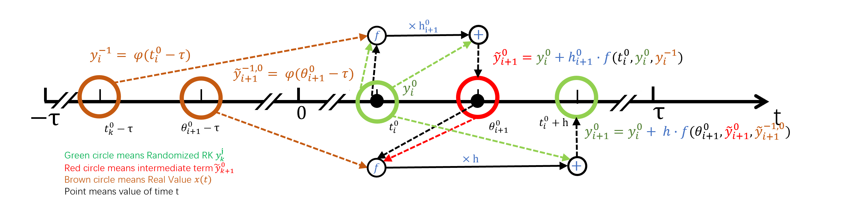
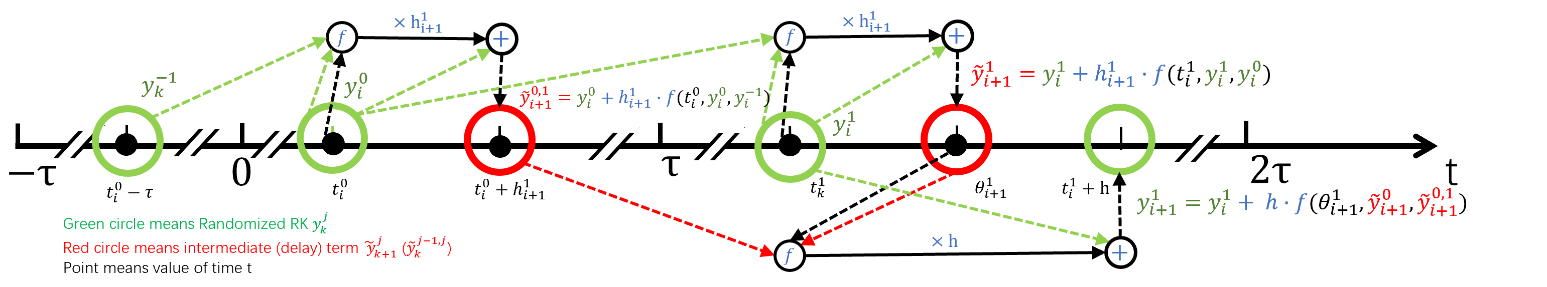
To help readers better understand the randomized RK method, we present two figures 1(a) and 1(b). Figure 1(a) depicts the scenario when , while Figure 1(b) showcases the situation for , using as a specific example. Within these figures, different markers are employed to convey distinct meanings: dashed lines represent assignments; black solid lines and solid circles signify computation methods; colored solid circles indicate the values of different terms at the time ; the black dots represent the value of time . For clarity, text is color-coded to match the terms they represent. Structurally, the figures are divided into two primary sections vertically along the coordinate axis. The upper section encompasses all computations excluding the generation of , while the lower section specifically illustrates the operations involved in generating . In both figures, for any in , we aim to compute the value of at the time point . We assume that the values of for all time points before are known. Utilizing these known values, we can calculate the value of at the time point using Eqn. (2.3) if or Eqn. (2.4) if .
3. Properties of solutions to Carathéodory DDEs
In this section we investigate the issue of existence and uniqueness of the solution of (1.1) under the assumptions (A1)-(A4).
In the sequel we use the following equivalent representation of the solution of (1.1), that is very convenient when proving its properties and when estimating the error of the randomized RK scheme. For and it holds
| (3.1) |
Hence, we take , and for we consider the following sequence of initial-value problems
| (3.2) |
with , . Then the solution of (1.1) can be written as
| (3.3) |
We prove the following result about existence, uniqueness and Hölder regularity of the solution of the delay differential equation (1.1). We will use this theorem in the next section when proving error estimate for the randomized RK algorithm.
Theorem 3.1.
Let , , and let , satisfy the assumptions (A1)-(A4). Then there exists a unique absolutely continuous solution to (1.1) such that for we have
| (3.4) |
where and
| (3.5) |
then for all , it holds
| (3.6) |
The proof of this theorem follows Theorem 3.1 from [9]. However, due to different initial conditions and assumptions, there are some subtle variations in the proof and conclusions. Specifically, the differences are as follows:
-
(1)
[9] considers a constant initial condition case, ie, for , while in our DDE, a general initial condition is taken, allowing the initial condition to vary with time.
- (2)
Remark 3.2.
Proof.
Follow the proof of Theorem 3.1 in [9], we proceed by induction. We start with the case when and consider the following initial-value problem.
| (3.7) |
with . It is obvious that for all the function is continuous and for all the function is Borel measurable. Moreover, by (2.1) we have
for all , and by (2.2) there exists such that for all , we have
| (3.8) |
Therefore, by Lemma 6.3 we have that there exists a unique absolutely continuous solution of (3.7) that satisfies (3.4) with . In addition, by Lemma 6.3 we obtain that satisfies (3.6) for . For the inductive step from to , we can simply follow the approach provided [9], since our assumptions (A3) and (A4) are stronger than [9, Assumptions A3 and A4]. It is crucial to note that [9, Eqn. (3.14)] will be modified to
4. Error of the randomized RK scheme
In this section we perform detailed error analysis for the randomized RK scheme. As mentioned in Section 1, for the error analysis we impose global Lipschitz assumption on with respect to together with global Hölder condition with respect to . Namely, instead of (A3) and (A4), we assume
-
(A3’)
there exist such that for all ,
(4.1) and there exist , such that:
1. for all , ,(4.2) 2. for all , ,
(4.3) 3. for all ,
(4.4)
Remark 4.1.
Lemma 4.2.
The function is bounded in norm for each , and is -Hölder continuous.
In particular, if the initial condition for , then is -Hölder continuous.
Proof.
The main result of this section is as follows.
Theorem 4.3.
Let , , , and let , satisfy the assumptions (A1), (A2), (A3’) for some and . There exist such that for all it holds
for ,
| (4.11) |
where .
Proof.
In the proof we use the following auxiliary notations: and . Then is uniformly distributed in and is uniformly distributed in . The latter one is a random stepsize uniformly distributed in .
We start with and consider the initial-vale problem (3.7). We define the auxiliary randomized Runge-Kutta (ARRK) scheme as
| (4.12) | ||||
as , for all we have that . That is to say, the ARRK scheme coincides with RRK scheme at .
From Lemma 4.2 it has been shown that is -Hölder continuous in time. Moreover, by (A1), (A2) and (A3’) we have that is Borel measurable, and for all and
| (4.13) | ||||
Hence, by Theorem 3.1 and by using analogous arguments as in the proof of Theorem 5.2 in [16], which guarantees (4.11), where does not depend on .
Let us now assume that there exists for which there exists such that for all
| (4.14) |
We consider the following initial-value problem
| (4.15) |
with . From Lemma 4.2 we know that is -Hölder continuous.
We define the ARRK scheme as follows
| (4.16) | ||||
From the definition it follows that , , , is measurable with respect to the -field generated by (2.5), as well as is . Moreover, approximates at , despite is not implementable. We use only in order to estimate the error (4.11) of , since it holds
| (4.17) | ||||
where for the last term we use the expression of the initial-value problem (4.15). Note that for . Now using (4.2), [regularity of f wrt time], and Theorem 3.1 to estimate the last term, one can obtain that
| (4.18) |
Thus, overall,
Taking the -norm on both sides gives that
| (4.19) | ||||
Note that via the Hölder inequality we get, for and all positive numbers , that
| (4.20) |
where is a generic constant, for any .
Now applying Gronwall inequality to (4.22) gives that
| (4.23) |
We now establish an upper bound on . For we have
| (4.24) | ||||
where
Since is -Hölder continuous from Lemma 4.2 and by (4.8) and (4.9) we get that
| (4.25) |
Then, by above inequity and Theorem 3.1 we get
| (4.26) |
Moreover, for the last term , by using (4.7) , we get
| (4.27) | ||||
Therefore, for all the following inequality holds
| (4.28) | ||||
| (4.29) |
where is a generic constant, for any .
In inequality (4.28), we utilize (4.14), (4.25), (4.26), and (4.27). Then, in inequality (4.29), we obtain the result by invoking (4.20).
By using Gronwall’s lemma, we get for all
which ends the inductive part of the proof. Finally, and the proof of (4.11) is finished. ∎
5. Numerical experiments
5.1. The implementation
The implementation of the randomized Runge-Kutta method is not straightforward. To evaluate the solution at time point within the interval for , we need four steps:
Step (j1): First simulate and set a random stepsize and a random time point .
Step (j2): Following the second line of (2.4), compute the intermediate delay term via the random stepsize, the time grid point and evaluations from the preceding -intervals, namely, and over , and within .
Step (j3): Following the third line of (2.4), compute the intermediate term via the random stepsize, the time grid point and previous evaluations from the preceding or the current -interval, namely, and within , and over .
Step (j4): Following the last line of (2.4), compute evaluation via the random time point, the preceding evaluation , the intermediate term and the intermediate delay term from Step (j1)-Step (j3).
5.2. Example 1
We modify [17, Example 6.2] as follows:
| (5.1) | ||||
where and
| (5.2) | ||||
Here we have three jump points at , and . Note that when , our proposed method can recover the performance shown in [17, Example 6.2], with an order of convergence roughly .
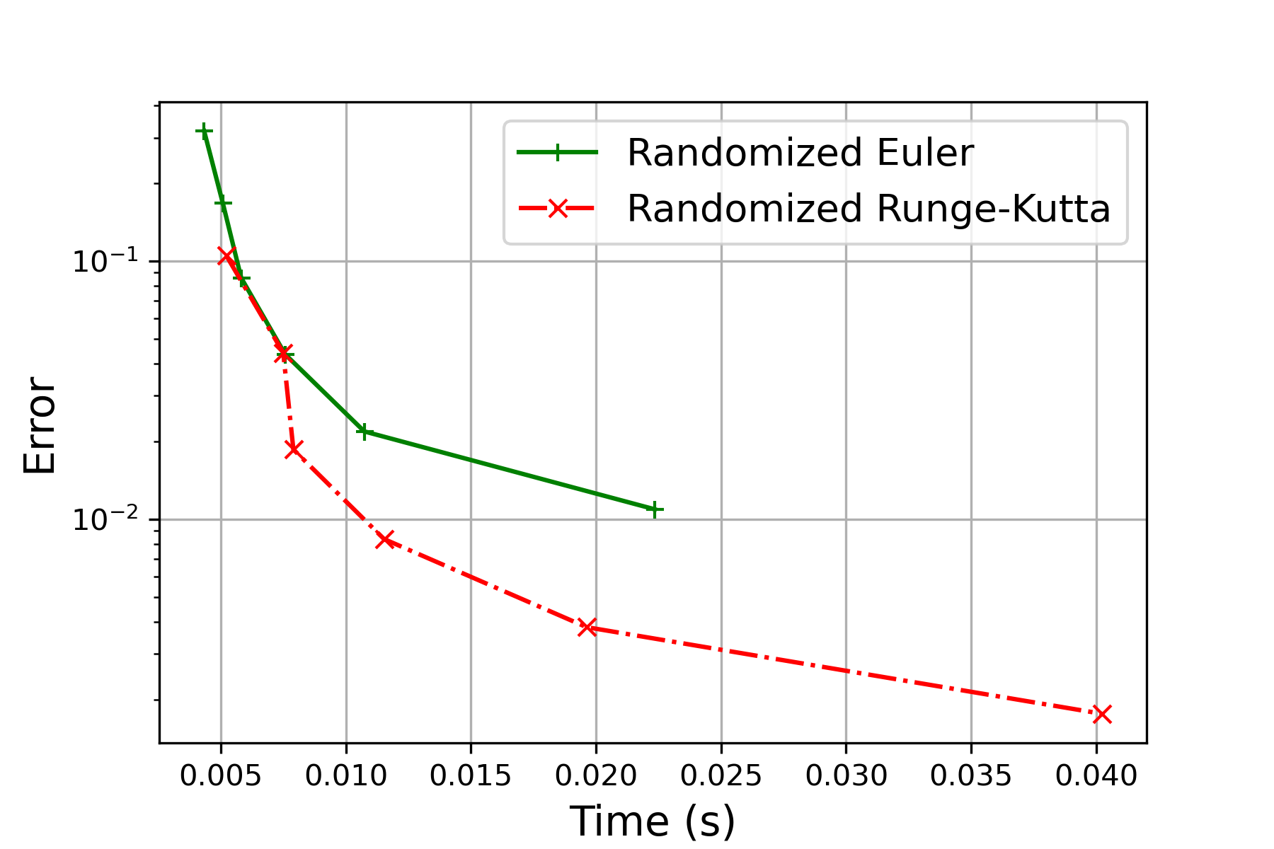
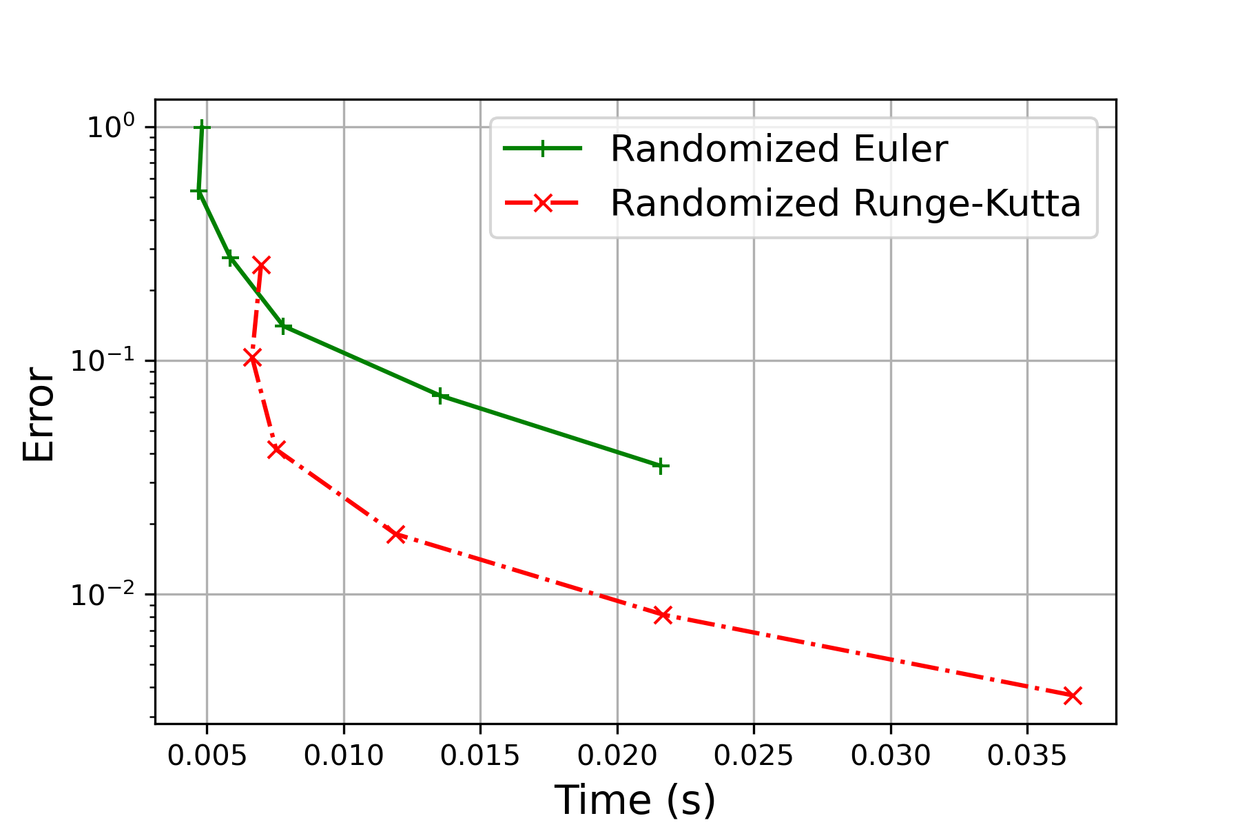
In this example, we choose and investigate the performance of our proposed method randomized Runge-Kutta method for solving such time-irregular DDE. The performance is further compared with the one of the randomized Euler method proposed in [9], which is known to efficiently handle Carathéodory DDEs, in terms of convergence rate, accuracy, and computational efficiency. The reference solution is computed through the randomized Runge-Kutta method at stepsize . We test the performance via experiments for each , , and record the mean-square error (MSE) and time cost against MSE for both methods respectively in Figure 2.
It can be observed from Figure 2(a) and Figure 2(b) that the randomized Runge-Kutta method outperforms consistently over all intervals in terms of accuracy and the order of convergence. Clearly, due to the additional computation of and in (2.4), the randomized Runge-Kutta method is approximately three times as expensive as the randomized Runge-Kutta method with the same step size. But due to its better accuracy, the randomized Runge-Kutta method is superior for all the step sizes smaller than .
5.3. Example 2
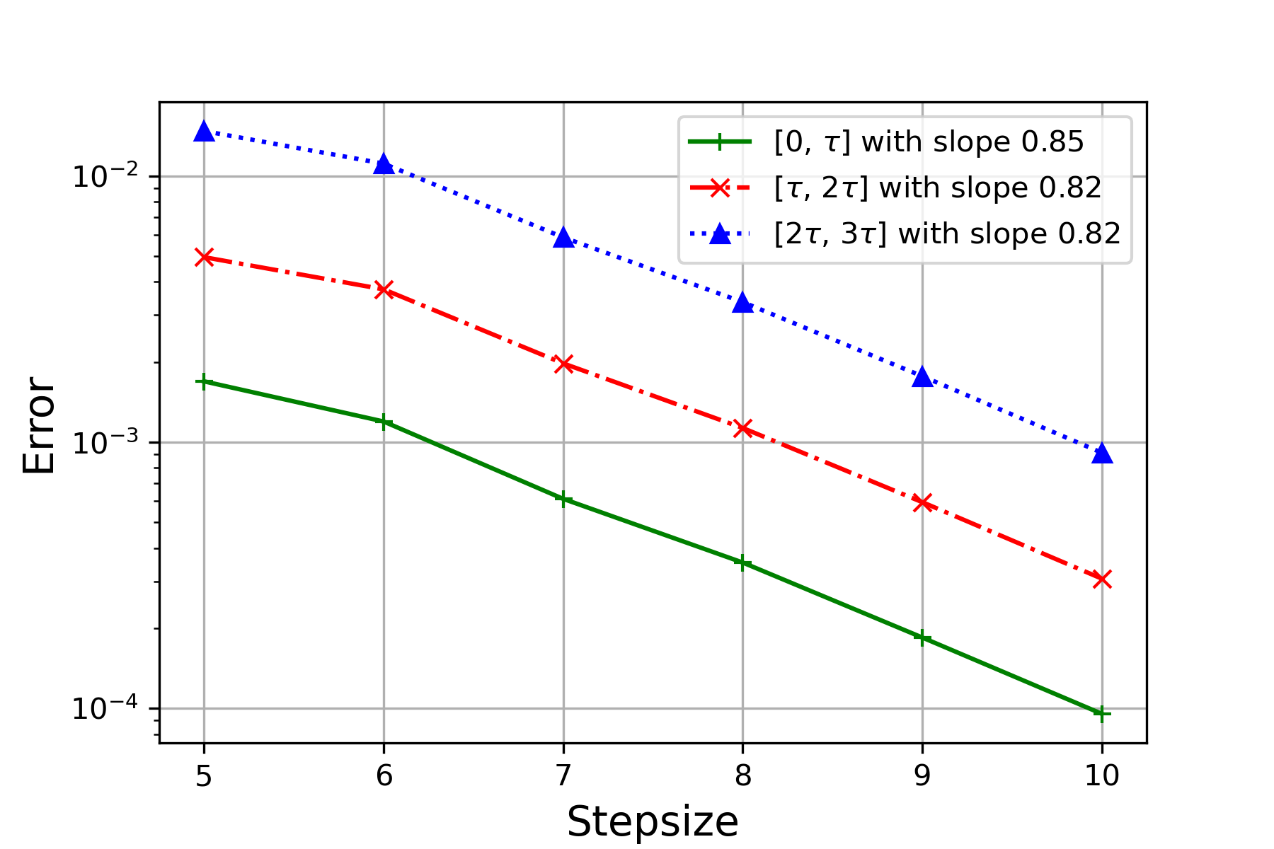
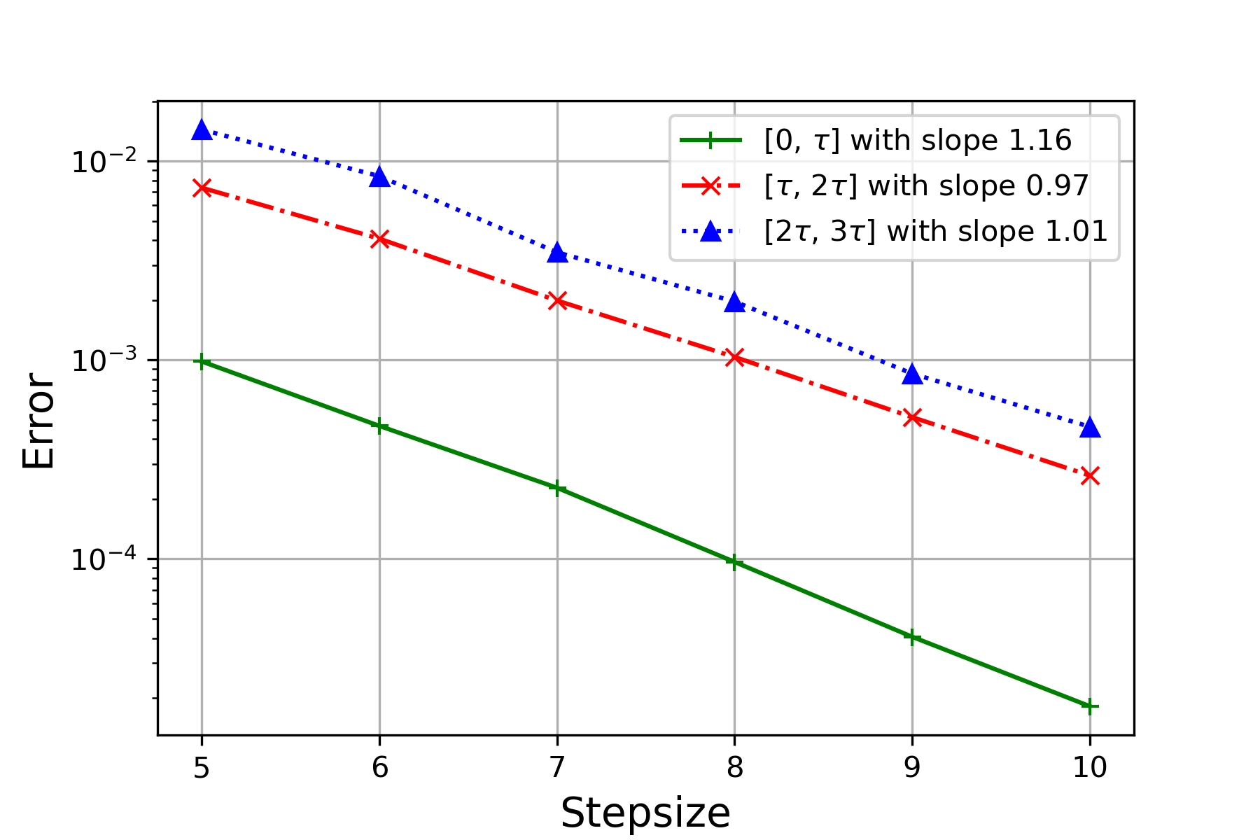
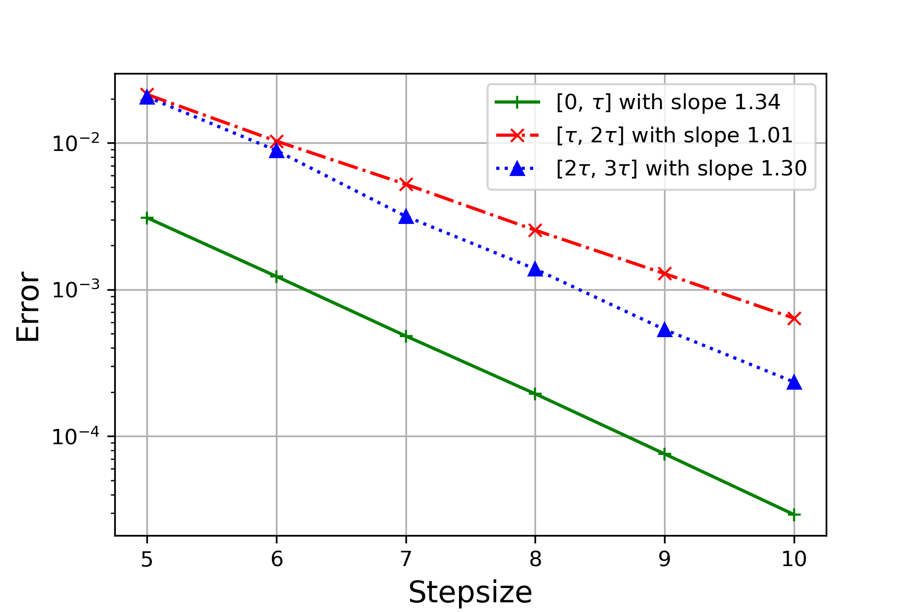
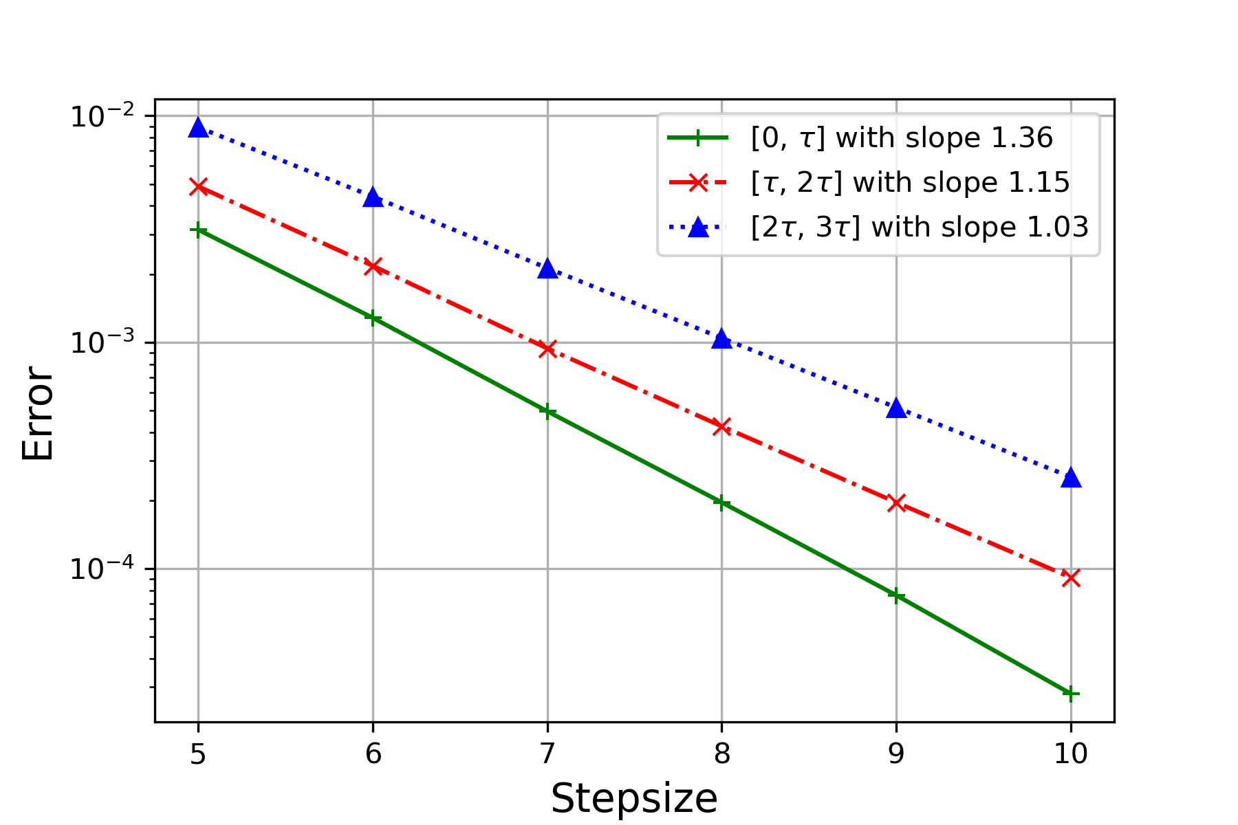
To verify (4.11) in Theorem 4.3, we test the sensitivity of the performance of the randomized Runge-Kutta method with respect to parameters on the following DDE:
| (5.3) | ||||
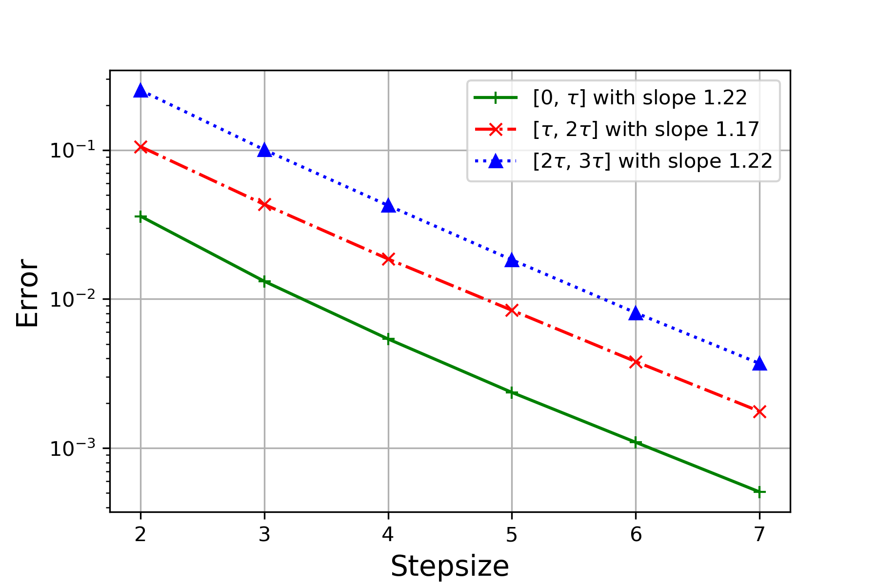
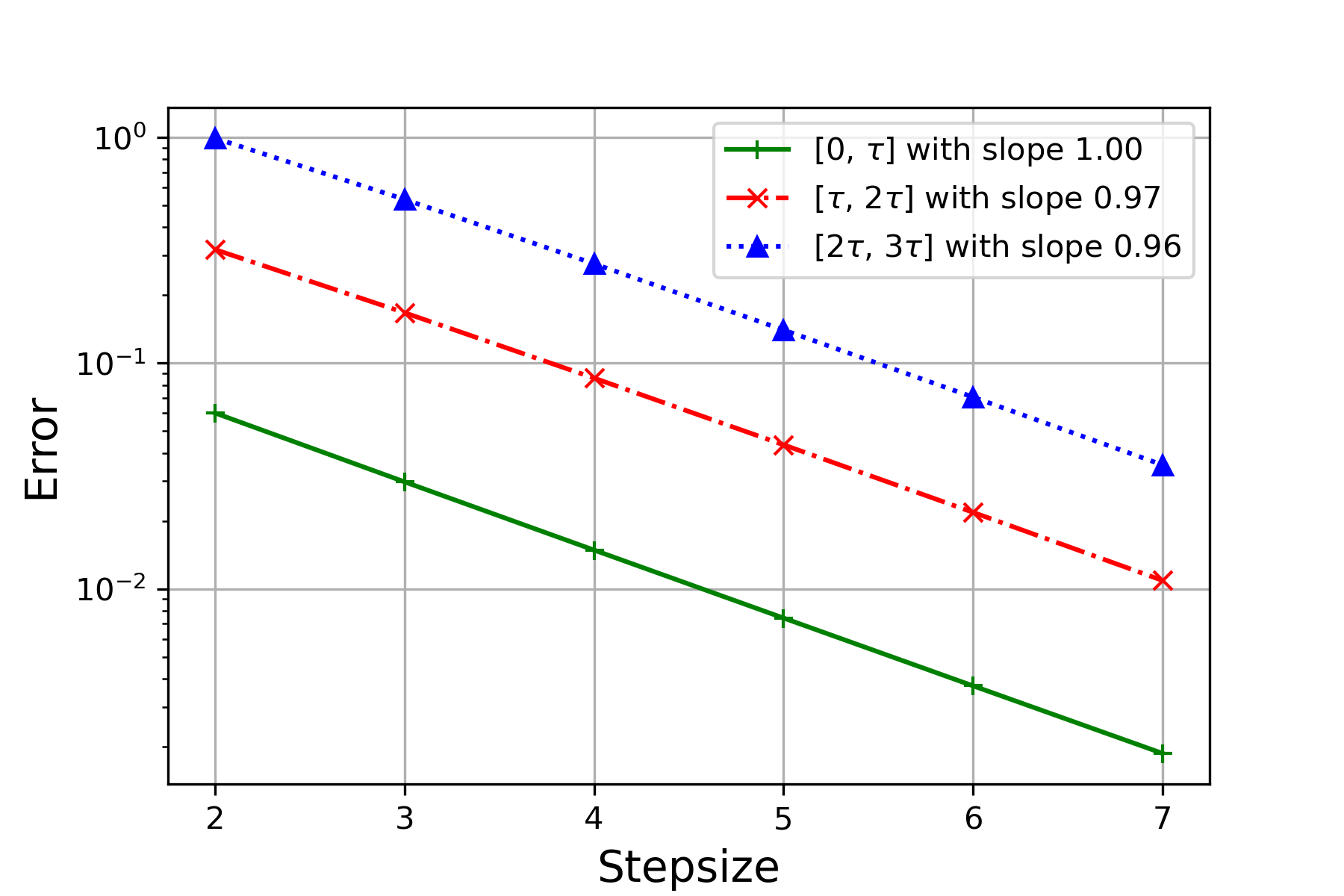
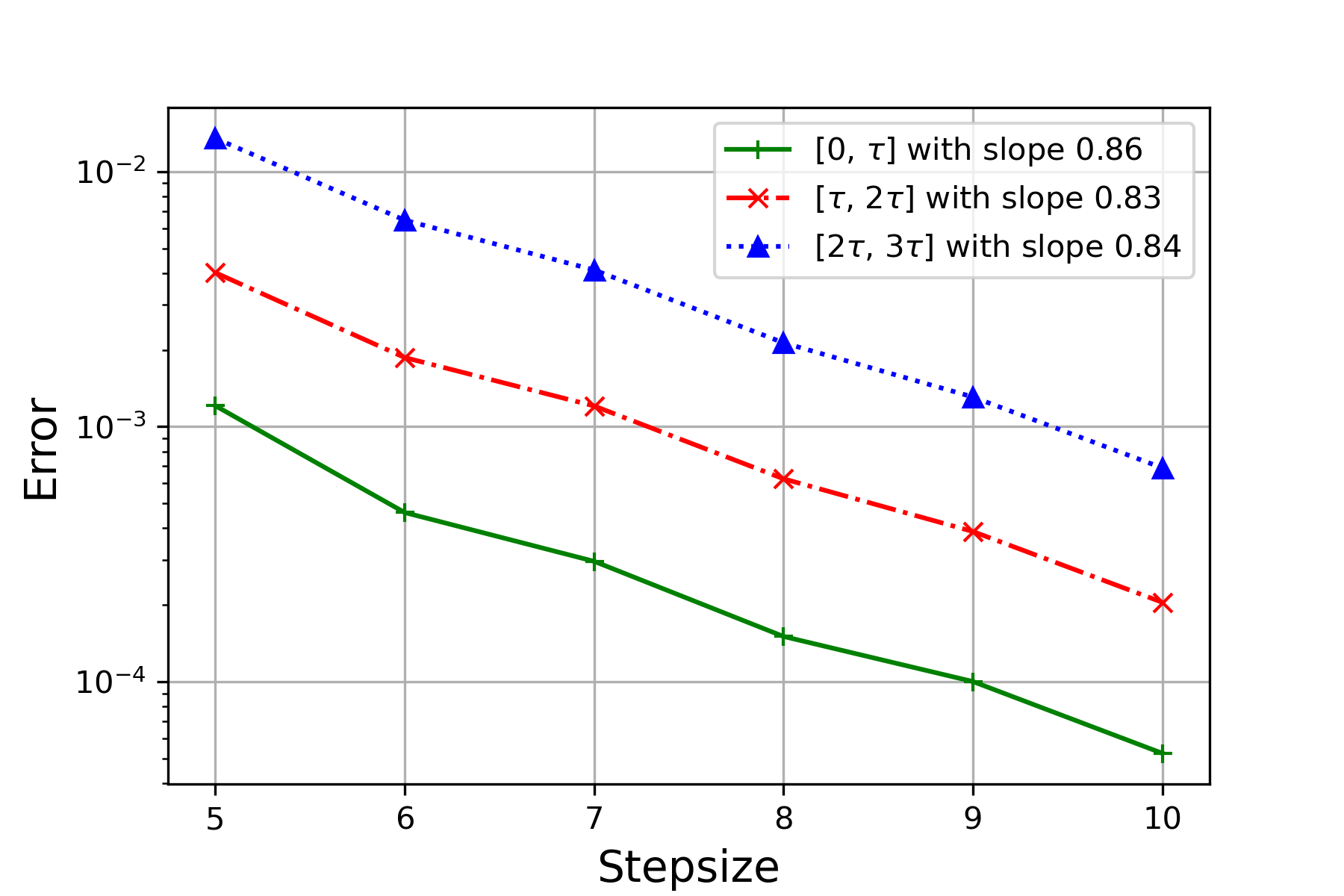
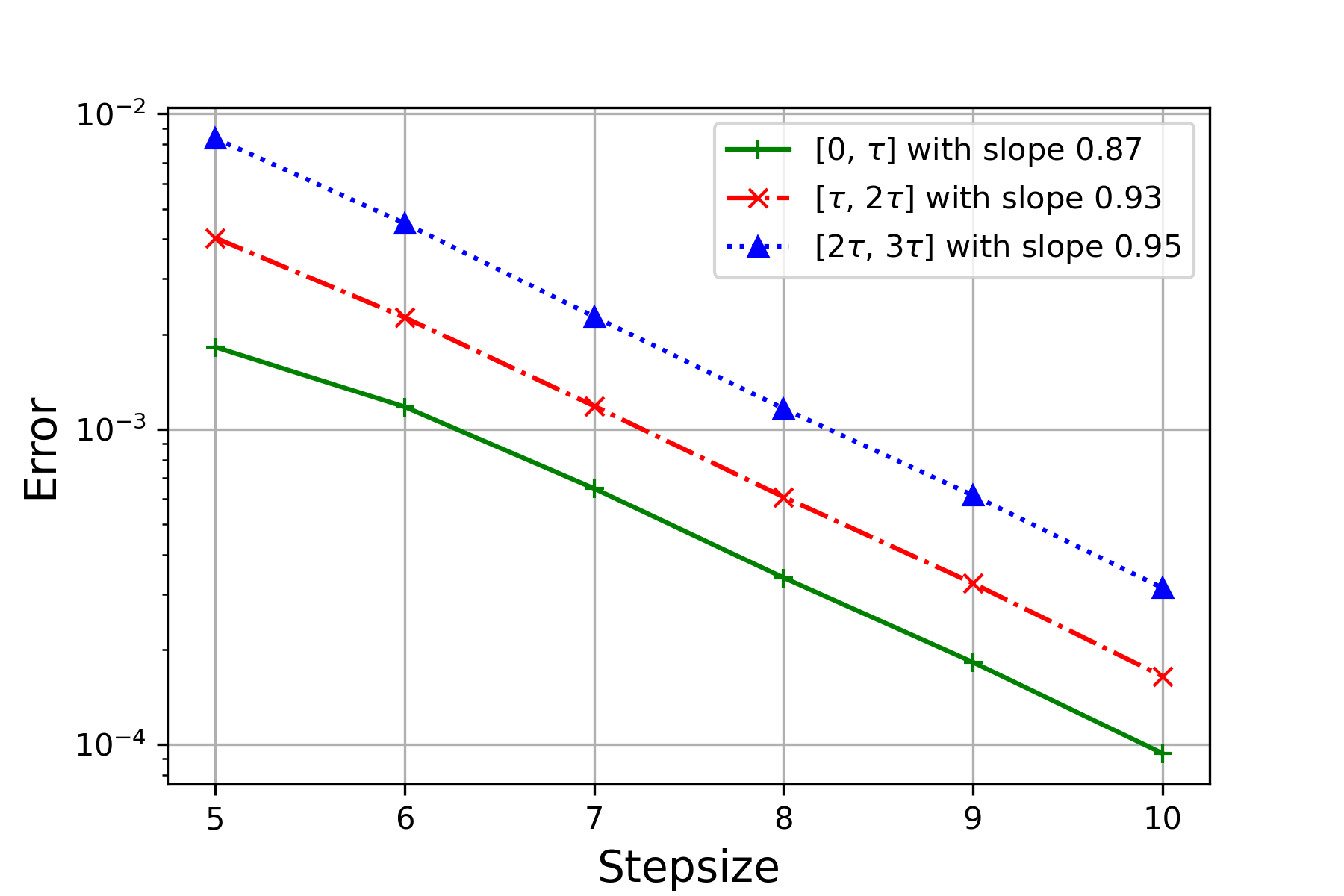
For each pair, the reference solution is computed through the randomized Runge-Kutta method at stepsize . We test the performance via experiments for each , , and record the mean-square error (MSE) and the negative MSE slope in Figure 3 and Table 1 respectively. One can observe from Table 1 that for each pair of , the order of convergence over is consistently higher than the theoretical one for , where the latter one is in (4.11). Particularly, it can been seen from Figure 3(a), Figure 3(b) and Figure 3(c) that, though orders of convergence from the three cases are similar over , the ones over and of Figure 3(b) are slightly higher than the other two, due to the larger value of . The result coincides with Theorem 4.3.
| Figure | |||||
|---|---|---|---|---|---|
| 0.1 | 0.1 | 0.86 | 0.83 | 0.84 | Figure 3(a) |
| 0.5 | 0.1 | 0.87 | 0.93 | 0.95 | Figure 3(b) |
| 0.1 | 0.5 | 0.85 | 0.82 | 0.82 | Figure 3(c) |
| 0.5 | 0.5 | 1.16 | 0.97 | 1.01 | Figure 3(d) |
| 0.5 | 1 | 1.34 | 1.01 | 1.30 | Figure 3(e) |
| 1 | 0.5 | 1.36 | 1.15 | 1.03 | Figure 3(f) |
6. Appendix
For the proof of the following continuous version of Gronwall’s lemma [20, pag. 22] see, for example, [19, pag. 580].
Lemma 6.1.
Let be an integrable function, be continuous on , and let be non-decreasing. If for all
| (6.1) |
then
| (6.2) |
We also use the following weighted discrete version of Gronwall’s inequality, see Lemma 2.1 in [16].
Lemma 6.2.
Consider two nonnegative sequences and which for some given satisfy
| (6.3) |
then for all it also holds true that
| (6.4) |
We use the following result concerning properties of solutions of Carathéodory ODEs. It follows from [1, Theorem 2.12] (compare also with [16, Proposition 4.2]).
Lemma 6.3.
Let us consider the following ODE
| (6.5) |
where , and satisfies the following conditions
-
(G1)
for all the function is continuous,
-
(G2)
for all the function is Borel measurable,
-
(G3)
there exists such that for all ,
-
(G4)
there exists such that for all ,
Then (6.5) has a unique absolutely continuous solution such that
| (6.6) |
Moreover, for all
| (6.7) |
where .
Proof.
The proof for our proposition follows the approach outlined in Lemma 7.1 of [9]. This is feasible because our assumptions (G3) and (G4) are stronger than [9, Assumptions (G3) and (G4)]. Particularly, [9, Eqn. (7.8) and Eqn. (7.9)] will undergo modifications as follows due to the strengthened conditions:
| (6.8) | ||||
Consequently, this gives rise to our refined conclusions. ∎
References
- [1] J. Andres and L. Górniewicz. Topological Fixed Point Principles for Boundary Value Problems, vol. I. Springer Science+Business Media Dordrecht, 2003.
- [2] A. Bellen and M. Zennaro. Numerical methods for delay differential equations. Oxford, New York, 2003.
- [3] T. Bochacik, M. Goćwin, P. M. Morkisz, and P. Przybyłowicz. Randomized Runge-Kutta method–Stability and convergence under inexact information. J. Complex., 65:101554, 2021.
- [4] T. Bochacik and P. Przybyłowicz. On the randomized Euler schemes for ODEs under inexact information. Numer. Algor., 91:1205–1229, 2022.
- [5] H. Brunner and E. Hairer. A general-purpose implicit-explicit Runge-Kutta integrator for delay differential equations. BIT Numerical Mathematics, 52(2):293–314, 2012.
- [6] N. Czyżewska, P. Morkisz, J. Kusiak, P. Oprocha, M. Pietrzyk, P. Przybyłowicz, Ł. Rauch, and D. Szeliga. On mathematical aspects of evolution of dislocation density in metallic materials. IEEE Access, 10:86793–86811, 2022.
- [7] N. Czyżewska, P. M. Morkisz, and P. Przybyłowicz. Approximation of solutions of DDEs under nonstandard assumptions via Euler scheme. Numer. Algor., 91:1829–1854, 2022.
- [8] T. Daun. On the randomized solution of initial value problems. J. Complex., 27:300–311, 2011.
- [9] Fabio V. Difonzo, Paweł Przybyłowicz, and Yue Wu. Existence, uniqueness and approximation of solutions to Carathéodory delay differential equations. Journal of Computational and Applied Mathematics, 436:115411, 2024.
- [10] C. A. Eulalia and C. Lubich. An analysis of multistep Runge-Kutta methods for delay differential equations. Mathematical and Computer Modelling, 34(10-11):1197–1213, 2001.
- [11] J. K. Hale. Theory of Functional Differential Equations. Applied Mathematical Sciences. Springer New York, 1977.
- [12] J. K. Hale and S. M. V. Lunel. Introduction to Functional Differential Equations. Springer-Verlag, New York, 1993.
- [13] S. Heinrich and B. Milla. The randomized complexity of initial value problems. J. Complex., 24:77–88, 2008.
- [14] A. Jentzen and A. Neuenkirch. A random Euler scheme for Carathéodory differential equations. J. Comp. Appl. Math., 224:346–359, 2009.
- [15] B. Kacewicz. Almost optimal solution of initial-value problems by randomized and quantum algorithms. J. Complex., 22:676–690, 2006.
- [16] R. Kruse and Y. Wu. Error analysis of randomized Runge–Kutta methods for differential equations with time-irregular coefficients. Comput. Methods Appl. Math., 17:479–498, 2017.
- [17] Raphael Kruse and Yue Wu. A randomized milstein method for stochastic differential equations with non-differentiable drift coefficients. arXiv preprint arXiv:1706.09964, 2017.
- [18] J. Kuehn. Numerical methods for delay differential equations. World Scientific Publishing Company, 2004.
- [19] E. Pardoux and A. Rascanu. Stochastic Differential Equations, Backward SDEs, Partial Differential Equations. Stochastic Modelling and Applied Probability. Springer International Publishing Switzerland, 2014.
- [20] E. Platen and N. Bruti-Liberati. Numerical Solution of Stochastic Differential Equations with Jumps in Finance. Stochastic Modelling and Applied Probability. Springer–Verlag Berlin Heidelberg, 2010.
- [21] Y. Song and X. Yang. A novel explicit two-stage Runge-Kutta method for delay differential equations with constant delay. Applied Mathematics and Computation, 272:317–322, 2015.