A Recipe for Unbounded Data Augmentation in
Visual Reinforcement Learning
Abstract
-learning algorithms are appealing for real-world applications due to their data-efficiency, but they are very prone to overfitting and training instabilities when trained from visual observations. Prior work, namely SVEA, finds that selective application of data augmentation can improve the visual generalization of RL agents without destabilizing training. We revisit its recipe for data augmentation, and find an assumption that limits its effectiveness to augmentations of a photometric nature. Addressing these limitations, we propose a generalized recipe, SADA, that works with wider varieties of augmentations. We benchmark its effectiveness on DMC-GB2 – our proposed extension of the popular DMControl Generalization Benchmark – as well as tasks from Meta-World and the Distracting Control Suite, and find that our method, SADA, greatly improves training stability and generalization of RL agents across a diverse set of augmentations.
Visualizations, code and benchmark: https://aalmuzairee.github.io/SADA
1 Introduction
Visual Reinforcement Learning (RL) has a myriad of real-world applications (Mnih et al., 2013; Levine et al., 2016; Pinto & Gupta, 2016; Kalashnikov et al., 2018; Berner et al., 2019; Vinyals et al., 2019), and visual -learning algorithms are especially enticing because of their potential for high data-efficiency. However, they are very prone to overfitting on their training distribution due to the combination of flexible representation, high-dimensional data, and limited visual diversity in training environments (Peng et al., 2018; Cobbe et al., 2019; Julian et al., 2020).
Data augmentation is a widely used technique for learning visual invariances in supervised learning (Noroozi & Favaro, 2016; Tian et al., 2019; Chen et al., 2020), but has been found to cause training instabilities when applied to visual RL (Lee et al., 2019; Laskin et al., 2020; Hansen & Wang, 2021). Prior work, SVEA (Hansen et al., 2021b), found that a more selective application of data augmentation in the critic update of actor-critic algorithms (Lillicrap et al., 2015; Haarnoja et al., 2018) improved training stability significantly. The actor (policy) – which shares its visual backbone with the critic (-function) – is then optimized solely from unaugmented observations. By sharing their visual backbone, the actor indirectly benefits from the learned invariances.
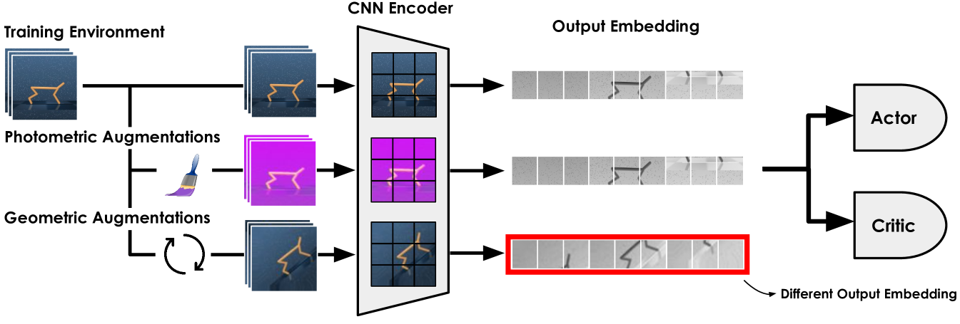
In this work, we revisit the data augmentation recipe proposed in SVEA, and discover an assumption that limits its practicality to augmentations of a photometric (color or light altering) nature. SVEA assumes that an encoder’s output embedding can become fully invariant to input augmentations. If an encoder’s output is fully invariant to input augmentations, then an actor, only trained on unaugmented observations, can become robust to input augmentations indirectly through a shared actor-critic encoder. However, this leads to two key failure cases: (i) the output of a convolutional neural network (CNN) encoder can not become invariant to input geometric augmentations e.g., rotation or translation; (see Figure 1) and (ii) the encoder and critic are trained end-to-end, thus, part of the invariance may be off-loaded to the critic regardless of the type of augmentation.
To address these limitations, we propose SADA: Stabilized Actor-Critic under Data Augmentation, a generalized data augmentation recipe that supports a wide variety of augmentations. Instead of only augmenting critic inputs, SADA augments both actor and critic inputs, but does so carefully to avoid training instabilities: (1) in actor updates, only the policy input is augmented while the -function input is left unaugmented, (2) in critic updates, only the online -function input is augmented while the target -function input is unaugmented, and (3) we jointly optimize components on both augmented and unaugmented data. Importantly, SADA requires no additional forward passes, losses, or parameters.
To stress-test our method, we propose DMC-GB2, an extension of the DeepMind Control Suite Generalization Benchmark (Hansen & Wang, 2021) that encompasses a wider and more challenging collection of test environments than existing benchmarks. We benchmark methods across DMC-GB2, tasks from Meta-World (Yu et al., 2020), and the Distracting Control Suite (Stone et al., 2021), and find that SADA greatly improves training stability and generalization of RL agents under a diverse set of augmentations.
2 Prior Work on Data Augmentation for Visual RL
The practice of learning visual invariances by augmenting data is ubiquitous in machine learning literature, and has been studied extensively in the context of supervised and self-supervised learning algorithms for computer vision problems (Noroozi & Favaro, 2016; Wu et al., 2018; Oord et al., 2018; Tian et al., 2019; Chen et al., 2020; He et al., 2022). More recently, use of augmentation has also been popularized in the context of visual RL. However, there is mounting evidence that much of the wisdom and practices developed in other areas (e.g. computer vision) do not translate to RL problems, presumably due to differences in learning objectives, datasets, and network architectures used. For example, while machine learning literature commonly considers a fixed dataset, RL algorithms are often trained on a non-stationary data distribution (replay buffer) that changes throughout training, and incoming data is typically a function of the current (behavioral) policy. As a result, RL datasets are often small and have limited diversity. This section provides an overview of prior work that leverages data augmentation to improve data-efficiency and generalization.
Improving data-efficiency with data augmentation. Much of the existing literature on visual RL leverages weak data augmentation (e.g. random crop or image shift) as a regularizer when data is limited, i.e., when data-efficiency is critical (Srinivas et al., 2020; Laskin et al., 2020; Kostrikov et al., 2020; Stooke et al., 2020; Yarats et al., 2021; Hansen et al., 2023), without particular emphasis on generalization or robustness to changes in the environment. For example, seminal works RAD (Laskin et al., 2020) and DrQ (Kostrikov et al., 2020) demonstrate that randomly cropping or shifting images, respectively, by a few pixels greatly improves data-efficiency and training stability of -learning algorithms – even when agents are trained and tested in the same environment. However, Laskin et al. (2020) simultaneously find that other types of augmentation (rotation, random convolution, masking) lead to training instabilities and a substantial decrease in data-efficiency.
Improving generalization with data augmentation. Visual generalization is a challenging but increasingly important problem in RL due to its limited data diversity. Multiple prior works aim to improve the training stability and generalization of RL algorithms by, e.g., proposing new types of augmentation (Lee et al., 2019; Wang et al., 2020; Hansen & Wang, 2021; Hansen et al., 2021b; Zhang & Guo, 2021; Wang et al., 2023), or introducing new (auxiliary) objectives (Raileanu et al., 2020; Hansen et al., 2021a; Wang et al., 2021; Fan et al., 2021; Yuan et al., 2022; Yang et al., 2024). For example, Lee et al. (2019) augment high-frequency content in observations using random convolution, Hansen & Wang (2021) randomly overlay observations with out-of-domain images, and Yang et al. (2024) adapt to camera changes at test-time using an auxiliary self-supervised objective and augmented data. Perhaps most importantly, SVEA (Hansen et al., 2021b) investigate why strong augmentations (such as those used in the aforementioned works) often destabilize training in an RL context, and propose an alternative method of applying augmentations that mitigate these instabilities. Our work builds upon SVEA and demonstrates that – while SVEA is robust to photometric augmentations – it largely fails when applied to (equally important) geometric augmentations.
We recommend the survey by Kirk et al. (2023) for a more comprehensive overview of prior work.
3 Background & Definitions
Visual Reinforcement Learning (RL) formulates interaction between an agent and its environment as a Partially Observable Markov Decision Process (POMDP) (Kaelbling et al., 1998). A POMDP can be formalized as a tuple , where is an unobservable state space, are observations from the environment (e.g., RGB images), are actions, is a transition function, is a task reward from a reward function , and is a discount factor. Throughout this work, we approximate the unobservable states by defining observations as a stack of the three most recent RGB frames for frames at time (Mnih et al., 2013). The goal is then to learn a policy such that the discounted sum of rewards is maximized (in expectation) when following the policy .
-Learning algorithms developed for visual RL generally estimate the optimal state-action value function with a neural network (denoted the critic). This is achieved by dynamic programming using the single-step Bellman error where is the temporal difference (TD) target . In practice, the -network used to compute is usually chosen to be an exponential moving average of the -function being learned (Lillicrap et al., 2015; Haarnoja et al., 2018). The policy is obtained by taking the action in the current dataset (replay buffer), which is typically estimated by training a separate actor network when is continuous. These two components – the actor and the critic – are iteratively updated by collecting data in the environment, appending it to a replay buffer , and optimizing with the following objectives using stochastic gradient descent:
| (1) | ||||
| (2) |
where gradients of the first objective are computed wrt. only, and gradients of the second objective are computed wrt. only. When learning from images, observations are commonly encoded using a shared convolutional encoder such that are redefined as and , with only being updated by the critic objective . Due to the recurrent and self-referential nature of Equations 1-2, -learning algorithms are often more data-efficient than other algorithm classes, but are very prone to training instabilities – especially when data augmentation is applied to observations.
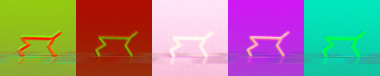
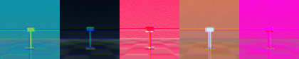
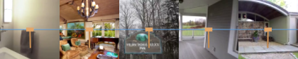
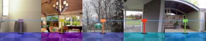
Image transformations. Throughout this work, we classify image transformations into two types: photometric and geometric transformations. Photometric transformations alter image color and lighting properties while preserving the spatial arrangement of pixels (e.g. random convolution, image overlay). Geometric transformations alter the spatial arrangement of pixels while keeping image color and lighting properties intact (e.g. rotation, shift). We visualize examples of photometric and geometric transformations in Figure 1.
4 Stabilized Actor-Critic Learning under Data Augmentation
We revisit common wisdom and practices when applying data augmentation in -learning algorithms, and discover that prior work makes an assumption that only holds for augmentations that are photometric in nature. We propose SADA: Stabilized Actor-Critic Learning under Data Augmentation, a generalized recipe for data augmentation that significantly improves the performance of a wider variety of augmentations. We start by outlining the assumptions of prior work, its implications, and then present our proposed solution.
4.1 Shortcomings of Prior Work
Naive augmentation, where all inputs are indiscriminately augmented, has been shown to lead policies to suboptimal convergence (Raileanu et al., 2020; Hansen et al., 2021b). Unlike supervised learning, the application of augmentation in RL can lead to a conflict of task objective, conflict of learning objective, or increased variance that exacerbates instabilities within actor-critic frameworks.
To stabilize actor-critic learning under strong applications of data augmentation, SVEA (Hansen et al., 2021b) selectively applies augmentations in the critic updates, without any application of augmentation in the actor updates. The actor – optimized purely from unaugmented observations – becomes robust to augmentations indirectly, through the use of a shared actor-critic encoder. By using this formulation, SVEA assumes that the encoder can output embeddings that are invariant to input augmentations, such that an actor can indirectly become robust to input augmentations. This assumption leads to two key failure cases: (i) the output embedding of a CNN encoder can not become invariant to input geometric augmentations, (ii) even with photometric augmentations, part of the robustness could be off-loaded to the critic.
We provide a motivating example for key failure case (i) in Figure 1 and show that geometric transformations will always induce changes in a CNN’s output embedding. Therefore, an actor not directly trained on these changed output embeddings will not become robust to these geometric transformations. As for key failure case (ii), a CNN can learn to output embeddings that are invariant to input photometric augmentations. However, the objective is formulated such that the output of the critic is robust to input image augmentations, indicating that if either the encoder or the critic is robust, the objective will be satisfied. Therefore, some of the photometric resistance might be contained within the critic, rendering the actor weaker against photometric transformations.
4.2 Our Proposed Recipe
To mitigate shortcomings of previous works, the actor needs to directly train on the augmented stream. However, naively training the actor on the augmented stream exacerbates training instabilities. Each image augmentation applied adds a more complex distribution for the agent to learn compared to the original training distribution. To overcome this complexity, we introduce SADA, a general framework for stabilizing actor-critic agents under strong applications of data augmentation.
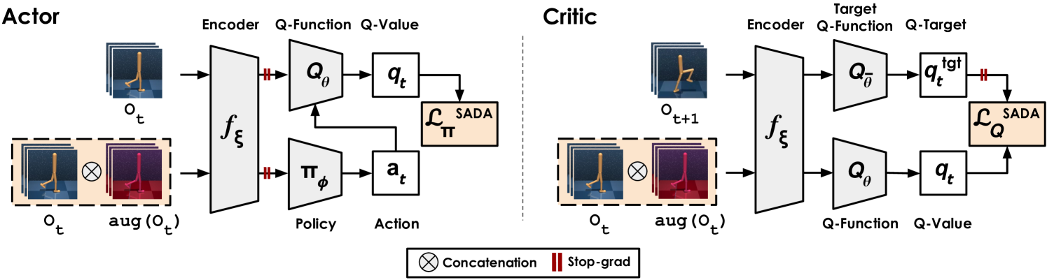
In the actor’s update, we elect to use asymmetric observation inputs to the policy and -function (Pinto et al., 2017). Specifically, we allow the policy to observe both the augmented and unaugmented streams, while the -function estimates the -value observing only the unaugmented stream. Since the -value estimates of both the augmented and unaugmented streams should be identical, we allow the -function to exploit only the unaugmented stream (easier distribution) in making accurate -value estimates. Given an observation , replay buffer , and an encoder , the actor objective for a generic actor critic thus becomes:
| (3) |
where and . We use to denote concatenation for batch size of dimensionality where . We use aug() as the augmentation operator where we stochastically sample from the augmentation distribution and apply it to the input observation.
In the critic update, we apply a similar asymmetric observation setup with the -value and -target estimates. We allow the online -function, , to estimate the -value observing both the augmented and unaugmented streams, while the target -function, , estimates the -targets observing only the unaugmented stream. Since the -target estimates of both the augmented and unaugmented streams should be identical, this reduces the variance in -target estimates and allows the target -function to exploit the unaugmented stream (easier distribution) in making accurate -target estimates. The -target estimate, , is unaltered while the critic objective, , is changed such that:
| (4) | ||||
| (5) |
where , and . An overview of our algorithm is provided in Figure 2. A detailed SAC-based formulation is provided in Appendix A.3, and pseudocode is provided in Appendix A.4.
5 Experiments
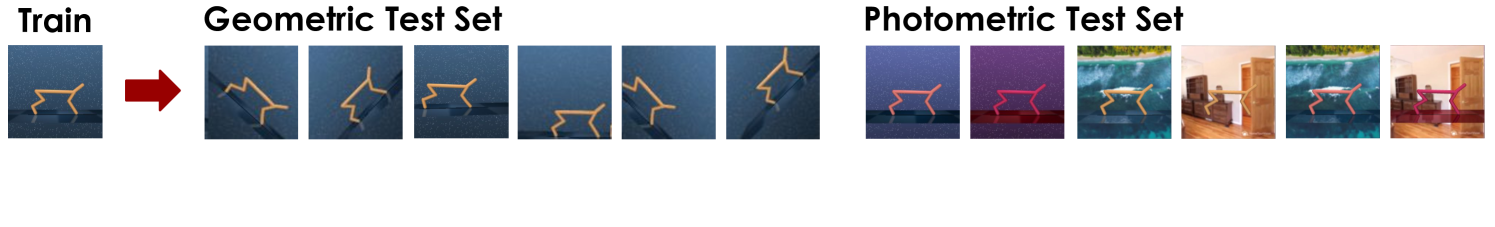
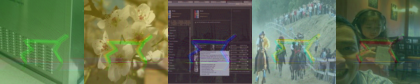
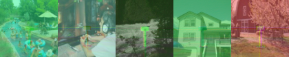
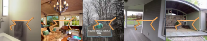
We evaluate our method and baselines across 11 visual RL tasks from the DMControl (Tassa et al., 2018) and Meta-World-v2 (Yu et al., 2020) benchmarks and 12 test distributions from our proposed DMControl - Generalization Benchmark 2 (DMC-GB2). We additionally evaluate on the Distracting Control Suite (Stone et al., 2021) and provide the results in Appendix B.2. All methods are trained under strong augmentations in the training environments and evaluated in a zero-shot manner on their respective test distributions. See Figure 3 for a visualization of DMC-GB2 test environments. The full DMControl and Meta-World task lists are provided in Appendix A.2. Concretely, we aim to answer the following questions through experimentation:
-
-
Robustness. How does SADA compare to baselines in terms of overall augmentation robustness? In terms of geometric vs photometric robustness?
-
-
Analysis. Why do baselines fail to display geometric robustness, and how does SADA solve the problem? How do each of the SADA design choices affect results?
-
-
Generality. Can SADA be readily applied to other RL backbones and benchmarks?
Setup. We build on DrQ (Laskin et al., 2020) as our backbone algorithm, and use a fixed set of hyperparameters across all tasks and environments. All agents are trained for one million environments steps and use stacks of the three most recent RGB frames ( as observations. A full list of hyperparameters and training details is provided in Appendix A.
Test environments. As our experiments will reveal, previous methods largely fail to generalize to geometric changes, which has gone unnoticed due to existing benchmarks predominantly evaluating photometric robustness. Therefore, we propose the Deepmind Control Suite Generalization Benchmark 2 (DMC-GB2), an extension of DMC-GB (Hansen & Wang, 2021) to encompass a wider collection of photometric and geometric test distributions. In DMC-GB2, we provide geometric and photometric test sets. The geometric test set considers two types of geometric distributions – rotations and shifts – both individually and jointly, and at varying intensities categorized as easy and hard environments. The photometric test set considers a complementary setup for two types of photometric distributions – colors and videos. Detailed visualizations of all 12 DMC-GB2 test distributions is provided in Appendix C.2.
Data augmentation. We apply a weak augmentation of random shifting to all our inputs as conducted in our DrQ baseline, and consider it unaugmented. We further employ a set of strong augmentations, taking into account both geometric and photometric transformations. For geometric augmentations, we use random shift (Laskin et al., 2020), random rotation, and a combination consisting of random rotation followed by random shift. For photometric augmentations we use random convolution (Lee et al., 2019), random overlay (Hansen & Wang, 2021), and a combination consisting of random convolution followed by random overlay. We sample an augmentation from this set of six strong augmentations for each input sample in all our experiments unless stated otherwise. Detailed visualizations of all augmentations is provided in Appendix C.1.
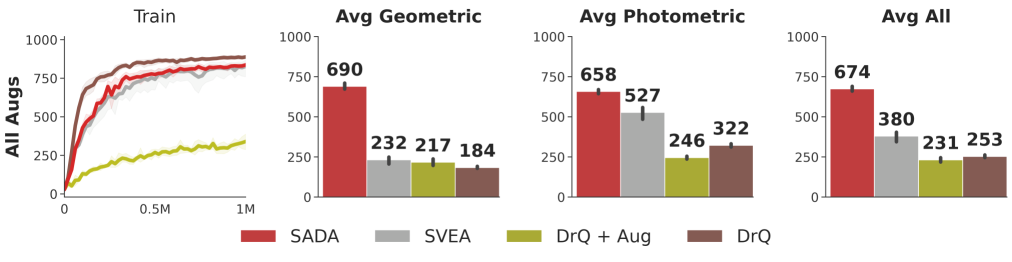
Baselines. We benchmark our method against the following well-established baselines. 1) DrQ Laskin et al. (2020), a visual based Soft Actor Critic baseline that uses random shifts as the default augmentation for all inputs. 2) DrQ + Aug, a variant of DrQ implemented with a naive application of strong augmentations. 3) SVEA Hansen et al. (2021b), which builds on DrQ with a selective application of augmentation in the -function to increase robustness under strong augmentations.
5.1 Results & Discussion
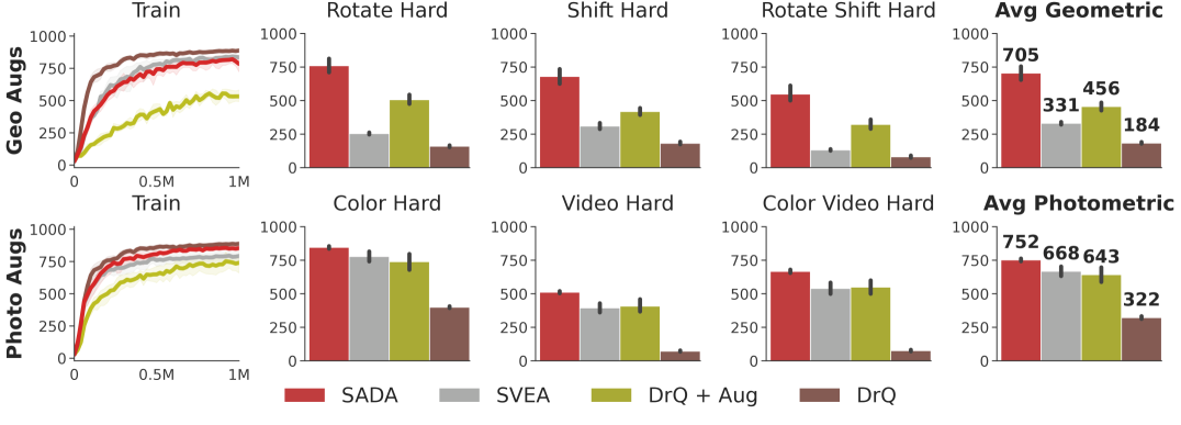
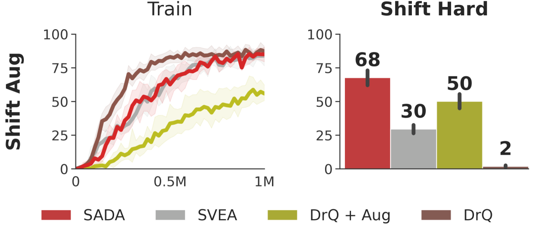
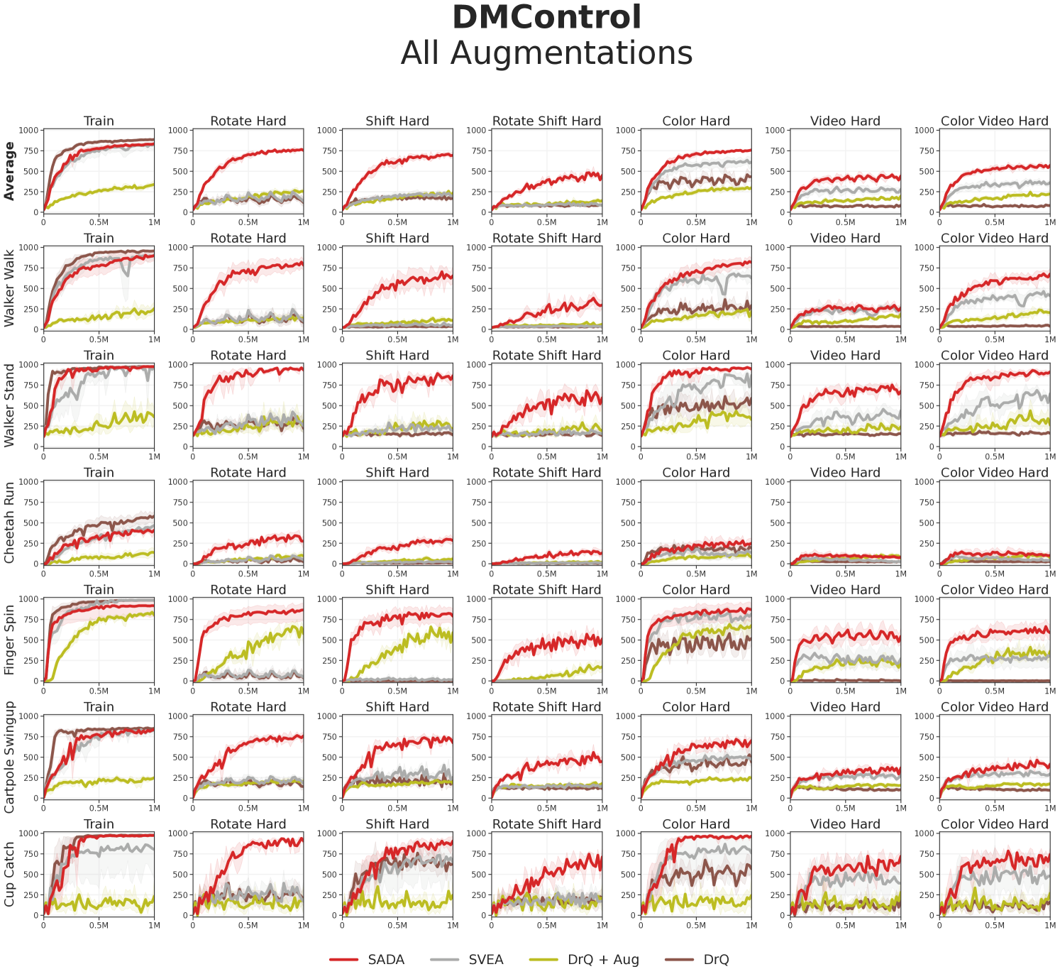
Robustness. For measuring the overall robustness, we train all methods under all augmentations (geometric and photometric augmentations) and evaluate them on all DMC-GB2 test sets (geometric and photometric test sets). As our empirical results indicate in Figure 3, SADA’s overall robustness surpasses the baselines in all DMC-GB2 test sets by a large margin (77%), all while attaining a similar sample efficiency to its unaugmented DrQ baseline on the training environment.
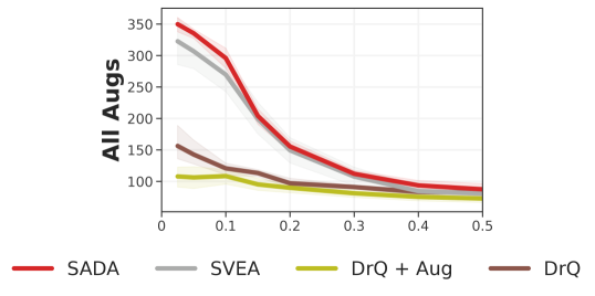
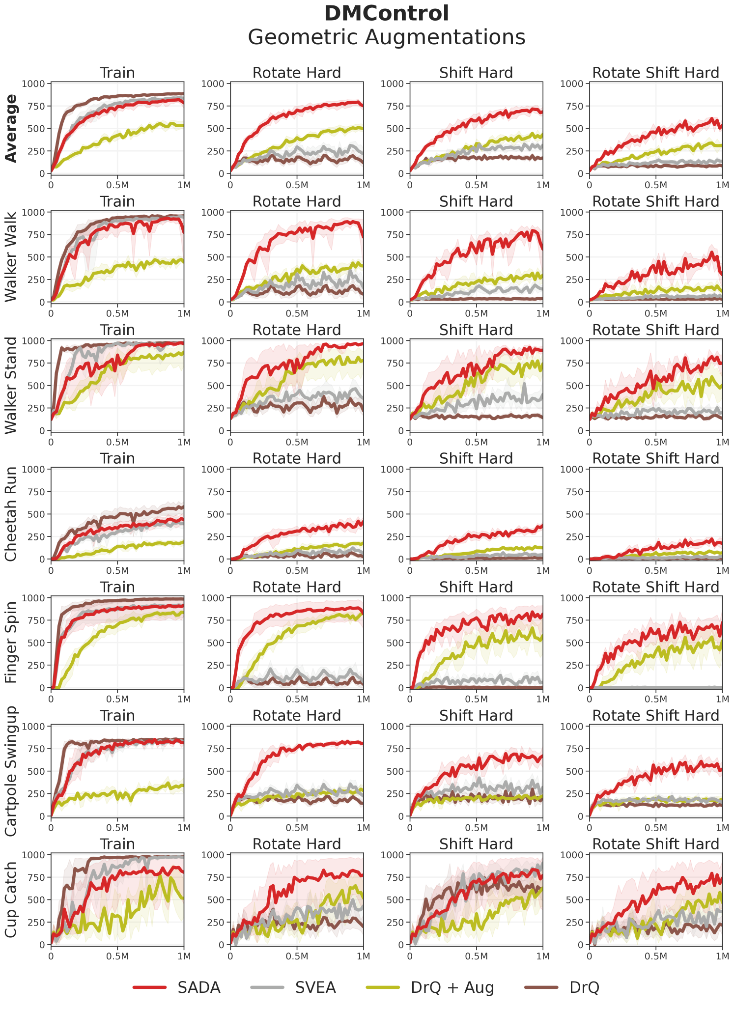
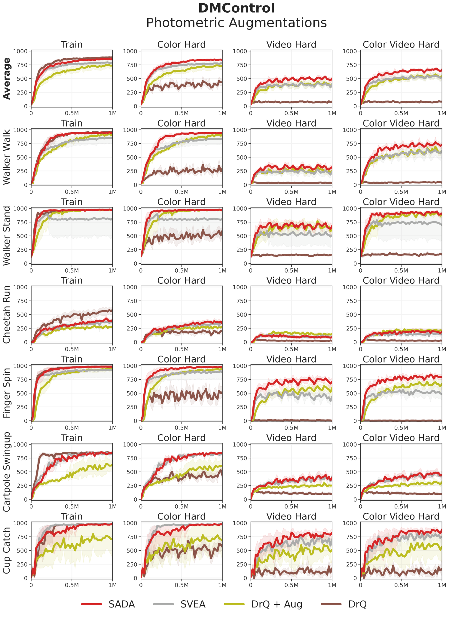
To analyze the geometric vs photometric robustness of each method, we conduct another experiment where we train under each set of augmentations separately. We train under strong geometric augmentations and evaluate on the geometric test set, and follow a complementary setup under strong photometric augmentations with the photometric test set. We visualize the results in Figure 4 along with all the individual hard level intensities in our test suite. SADA consistently shows superior robustness, outperforming baselines in all separate test sets and individual levels while achieving similar training sample efficiency to its unaugmented DrQ baseline. Extended results and per-task breakdowns are provided in Appendix D.
Analysis. While baselines show varying degrees of photometric robustness, they fail to display geometric robustness in Figures 3 and 4. For the DrQ baseline, geometric transformations are out of its training distribution. With naive application of data augmentation, DrQ + Aug achieves poor training sample efficiency. To achieve high training sample efficiency, SVEA selectively applies augmentation in the critic update. Nevertheless, this performance does not translate to the geometric test distributions due to key failure case (i), the output embedding of a CNN can not become invariant to input geometric transformations. This failure case can only be resolved with an actor directly trained on the input augmentations. When the actor is directly trained on the input augmentations using SADA’s objective, the agent is able to achieve high training sample efficiency that effectively translates to the geometric test distributions.
Even in terms of photometric robustness, SADA surpasses all baselines, including SVEA. This is mainly due to failure case (ii) of SVEA’s assumption, where some of the augmentation robustness is contained within the critic and not the encoder. This can also be resolved by training the actor directly on the input augmentations using SADA’s objective.
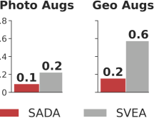
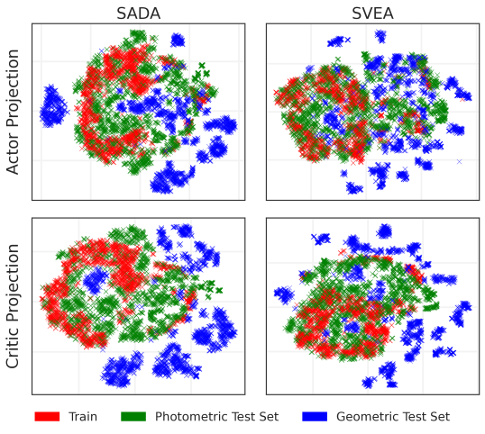
To quantitatively assess the augmentation robustness of converged SADA and SVEA agents, we measure the variance of actions predicted on the augmented observations with respect to the unaugmented observations in Figure 5. Despite being trained on all augmentations, SVEA’s action predictions have high variance when observing geometric augmentations as opposed to photometric augmentations, confirming SVEA’s shortcomings. For a qualitative assessment, we utilize T-SNE to visualize the encoder’s output embedding before being fed into the actor and the critic in Appendix B.3. Our findings reveal that photometric distributions can share the same space in the latent embedding as the original training distribution, while geometric distributions are distant in the latent space and seem to have little overlap with the training distribution, necessitating the need to directly train the actor on them.
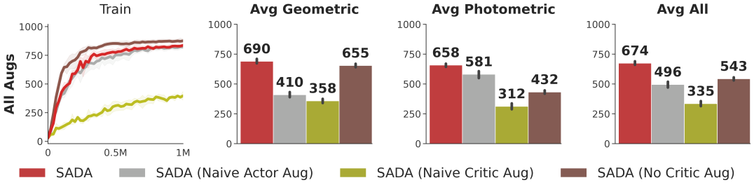
We ablate each of our design choices, evaluating methods under all augmentations on all DMC-GB2 test sets, and show results in Figure 6. Naively applying augmentation to the actor or the critic, as displayed in SADA (Naive Actor Aug) and SADA (Naive Critic Aug) respectively, leads to deteriorated performance. As for SADA (No Critic Aug), we only apply augmentation to the actor using SADA’s objective without any application of augmentation to the critic. SADA (No Critic Aug) displays impressive geometric robustness and training sample efficiency, but lacks in photometric robustness. If a user is only interested in geometric robustness, SADA (No Critic Aug) provides commendable geometric robustness. Overall, each of our design choices play a key role in establishing the superiority of SADA in all applications of data augmentation.
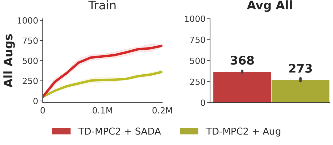
Generality. To demonstrate the generality of our approach, we swap our DrQ backbone with TD-MPC2 (Hansen et al., 2022; 2024), a state-of-the-art model-based RL algorithm; results are shown in Figure 8. We observe that SADA similarly improves training stability and generalization of TD-MPC2 on DMC-GB2.
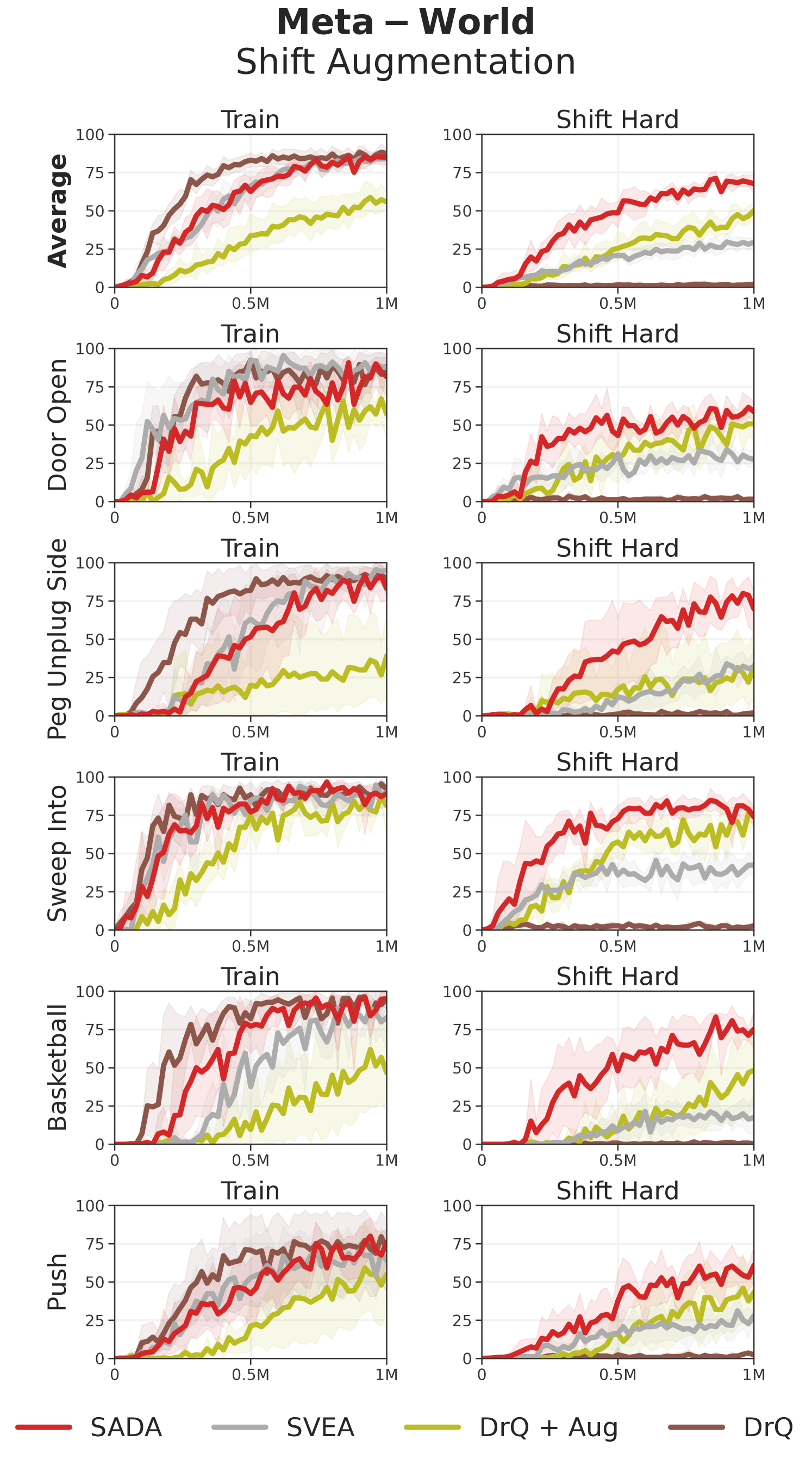
We further evaluate our DrQ-based SADA on our Meta-World setup (see Appendix C.3), and showcase the results in Figure 8. Even on Meta-World, SADA surpasses all other baselines in terms of success rate, all while achieving similar training sample efficiency to its unaugmented DrQ baseline. This asserts that SADA can be readily applied to diverse tasks, environments, and backbones, and can be used a generic data augmentation strategy for modern visual based reinforcement learning.
6 Summary
Throughout this work, we give an overview of data augmentation within visual RL, highlighting the shortcomings of previous work, its implications, and presenting SADA, a generic data augmentation recipe for modern visual based reinforcement learning. We empirically prove SADA’s superiority to previous methods and provide a deep analysis of its effectiveness. Concurrently, we curated a comprehensive visual generalization benchmark, DMC-GB2, which we make publicly available at https://aalmuzairee.github.io/SADA, with the aim of furthering research efforts within visual RL.
References
- Berner et al. (2019) Christopher Berner, Greg Brockman, Brooke Chan, Vicki Cheung, Przemyslaw Debiak, Christy Dennison, David Farhi, Quirin Fischer, et al. Dota 2 with large scale deep reinforcement learning. ArXiv, abs/1912.06680, 2019.
- Chen et al. (2020) Ting Chen, Simon Kornblith, Mohammad Norouzi, and Geoffrey Hinton. A simple framework for contrastive learning of visual representations. In International conference on machine learning, pp. 1597–1607. PMLR, 2020.
- Cobbe et al. (2019) Karl Cobbe, Oleg Klimov, Chris Hesse, Taehoon Kim, and John Schulman. Quantifying generalization in reinforcement learning. In International conference on machine learning, pp. 1282–1289. PMLR, 2019.
- Fan et al. (2021) Linxi Fan, Guanzhi Wang, De-An Huang, Zhiding Yu, Li Fei-Fei, Yuke Zhu, and Animashree Anandkumar. Secant: Self-expert cloning for zero-shot generalization of visual policies. In Marina Meila and Tong Zhang (eds.), Proceedings of the 38th International Conference on Machine Learning, volume 139 of Proceedings of Machine Learning Research, pp. 3088–3099. PMLR, 18–24 Jul 2021.
- Haarnoja et al. (2018) Tuomas Haarnoja, Aurick Zhou, Pieter Abbeel, and Sergey Levine. Soft actor-critic: Off-policy maximum entropy deep reinforcement learning with a stochastic actor. arXiv preprint arXiv:1801.01290, 2018.
- Hansen & Wang (2021) Nicklas Hansen and Xiaolong Wang. Generalization in reinforcement learning by soft data augmentation. In International Conference on Robotics and Automation, 2021.
- Hansen et al. (2021a) Nicklas Hansen, Rishabh Jangir, Yu Sun, Guillem Alenyà, Pieter Abbeel, Alexei A. Efros, Lerrel Pinto, and Xiaolong Wang. Self-supervised policy adaptation during deployment. In International Conference on Learning Representations, 2021a.
- Hansen et al. (2021b) Nicklas Hansen, Hao Su, and Xiaolong Wang. Stabilizing deep q-learning with convnets and vision transformers under data augmentation. In Annual Conference on Neural Information Processing Systems (NeurIPS), 2021b.
- Hansen et al. (2022) Nicklas Hansen, Xiaolong Wang, and Hao Su. Temporal difference learning for model predictive control. In International Conference on Machine Learning (ICML), 2022.
- Hansen et al. (2023) Nicklas Hansen, Zhecheng Yuan, Yanjie Ze, Tongzhou Mu, Aravind Rajeswaran, Hao Su, Huazhe Xu, and Xiaolong Wang. On pre-training for visuo-motor control: Revisiting a learning-from-scratch baseline. In International Conference on Machine Learning (ICML), 2023.
- Hansen et al. (2024) Nicklas Hansen, Hao Su, and Xiaolong Wang. TD-MPC2: Scalable, robust world models for continuous control. In International Conference on Learning Representations (ICLR), 2024.
- He et al. (2022) Kaiming He, Xinlei Chen, Saining Xie, Yanghao Li, Piotr Dollár, and Ross Girshick. Masked autoencoders are scalable vision learners. In Proceedings of the IEEE/CVF conference on computer vision and pattern recognition, pp. 16000–16009, 2022.
- Julian et al. (2020) Ryan C. Julian, Benjamin Swanson, Gaurav S. Sukhatme, Sergey Levine, Chelsea Finn, and Karol Hausman. Efficient adaptation for end-to-end vision-based robotic manipulation. ArXiv, abs/2004.10190, 2020.
- Kaelbling et al. (1998) Leslie Pack Kaelbling, Michael L. Littman, and Anthony R. Cassandra. Planning and acting in partially observable stochastic domains. Artificial Intelligence, 1998.
- Kalashnikov et al. (2018) Dmitry Kalashnikov, Alex Irpan, Peter Pastor, Julian Ibarz, Alexander Herzog, Eric Jang, Deirdre Quillen, Ethan Holly, Mrinal Kalakrishnan, Vincent Vanhoucke, et al. Qt-opt: Scalable deep reinforcement learning for vision-based robotic manipulation. arXiv preprint arXiv:1806.10293, 2018.
- Kirk et al. (2023) Robert Kirk, Amy Zhang, Edward Grefenstette, and Tim Rocktäschel. A survey of zero-shot generalisation in deep reinforcement learning. Journal of Artificial Intelligence Research, 76:201–264, 2023.
- Kostrikov et al. (2020) Ilya Kostrikov, Denis Yarats, and Rob Fergus. Image augmentation is all you need: Regularizing deep reinforcement learning from pixels. International Conference on Learning Representations, 2020.
- Laskin et al. (2020) Michael Laskin, Kimin Lee, Adam Stooke, Lerrel Pinto, Pieter Abbeel, and Aravind Srinivas. Reinforcement learning with augmented data. arXiv preprint arXiv:2004.14990, 2020.
- Lee et al. (2019) Kimin Lee, Kibok Lee, Jinwoo Shin, and Honglak Lee. A simple randomization technique for generalization in deep reinforcement learning. ArXiv, abs/1910.05396, 2019.
- Levine et al. (2016) Sergey Levine, Chelsea Finn, Trevor Darrell, and Pieter Abbeel. End-to-end training of deep visuomotor policies. The Journal of Machine Learning Research, 17(1):1334–1373, 2016.
- Lillicrap et al. (2015) Timothy P Lillicrap, Jonathan J Hunt, Alexander Pritzel, Nicolas Heess, Tom Erez, Yuval Tassa, David Silver, and Daan Wierstra. Continuous control with deep reinforcement learning. arXiv preprint arXiv:1509.02971, 2015.
- Mnih et al. (2013) Volodymyr Mnih, Koray Kavukcuoglu, David Silver, Alex Graves, Ioannis Antonoglou, Daan Wierstra, and Martin Riedmiller. Playing atari with deep reinforcement learning. arXiv preprint arXiv:1312.5602, 2013.
- Noroozi & Favaro (2016) Mehdi Noroozi and Paolo Favaro. Unsupervised learning of visual representations by solving jigsaw puzzles. In European Conference on Computer Vision, pp. 69–84. Springer, 2016.
- Oord et al. (2018) Aaron van den Oord, Yazhe Li, and Oriol Vinyals. Representation learning with contrastive predictive coding. arXiv preprint arXiv:1807.03748, 2018.
- Peng et al. (2018) Xue Bin Peng, Marcin Andrychowicz, Wojciech Zaremba, and Pieter Abbeel. Sim-to-real transfer of robotic control with dynamics randomization. 2018 IEEE International Conference on Robotics and Automation (ICRA), May 2018.
- Pinto & Gupta (2016) Lerrel Pinto and Abhinav Gupta. Supersizing self-supervision: Learning to grasp from 50k tries and 700 robot hours. In 2016 IEEE international conference on robotics and automation (ICRA), pp. 3406–3413. IEEE, 2016.
- Pinto et al. (2017) Lerrel Pinto, Marcin Andrychowicz, Peter Welinder, Wojciech Zaremba, and Pieter Abbeel. Asymmetric actor critic for image-based robot learning. arXiv preprint arXiv:1710.06542, 2017.
- Raileanu et al. (2020) Roberta Raileanu, M. Goldstein, Denis Yarats, Ilya Kostrikov, and R. Fergus. Automatic data augmentation for generalization in deep reinforcement learning. ArXiv, abs/2006.12862, 2020.
- Seo et al. (2023) Younggyo Seo, Danijar Hafner, Hao Liu, Fangchen Liu, Stephen James, Kimin Lee, and Pieter Abbeel. Masked world models for visual control. In Conference on Robot Learning, pp. 1332–1344. PMLR, 2023.
- Srinivas et al. (2020) Aravind Srinivas, Michael Laskin, and Pieter Abbeel. Curl: Contrastive unsupervised representations for reinforcement learning. arXiv preprint arXiv:2004.04136, 2020.
- Stone et al. (2021) Austin Stone, Oscar Ramirez, Kurt Konolige, and Rico Jonschkowski. The distracting control suite–a challenging benchmark for reinforcement learning from pixels. arXiv preprint arXiv:2101.02722, 2021.
- Stooke et al. (2020) Adam Stooke, Kimin Lee, Pieter Abbeel, and Michael Laskin. Decoupling representation learning from reinforcement learning. ArXiv, abs/2004.1499, 2020.
- Tassa et al. (2018) Yuval Tassa, Yotam Doron, Alistair Muldal, Tom Erez, Yazhe Li, Diego de Las Casas, David Budden, Abbas Abdolmaleki, Josh Merel, Andrew Lefrancq, et al. Deepmind control suite. arXiv preprint arXiv:1801.00690, 2018.
- Tian et al. (2019) Yonglong Tian, Dilip Krishnan, and Phillip Isola. Contrastive multiview coding. arXiv preprint arXiv:1906.05849, 2019.
- Vinyals et al. (2019) Oriol Vinyals, I. Babuschkin, Wojciech Czarnecki, Michaël Mathieu, Andrew Dudzik, J. Chung, D. Choi, Richard Powell, et al. Grandmaster level in starcraft ii using multi-agent reinforcement learning. Nature, pp. 1–5, 2019.
- Wang et al. (2020) Kaixin Wang, Bingyi Kang, Jie Shao, and Jiashi Feng. Improving generalization in reinforcement learning with mixture regularization. Advances in Neural Information Processing Systems, 33:7968–7978, 2020.
- Wang et al. (2021) Xudong Wang, Long Lian, and Stella X. Yu. Unsupervised visual attention and invariance for reinforcement learning. ArXiv, abs/2104.02921, 2021.
- Wang et al. (2023) Ziyu Wang, Yanjie Ze, Yifei Sun, Zhecheng Yuan, and Huazhe Xu. Generalizable visual reinforcement learning with segment anything model. arXiv preprint arXiv:2312.17116, 2023.
- Wu et al. (2018) Zhirong Wu, Yuanjun Xiong, Stella X Yu, and Dahua Lin. Unsupervised feature learning via non-parametric instance discrimination. In Proceedings of the IEEE Conference on Computer Vision and Pattern Recognition, pp. 3733–3742, 2018.
- Yang et al. (2024) Sizhe Yang, Yanjie Ze, and Huazhe Xu. Movie: Visual model-based policy adaptation for view generalization. Advances in Neural Information Processing Systems, 36, 2024.
- Yarats et al. (2021) Denis Yarats, Rob Fergus, Alessandro Lazaric, and Lerrel Pinto. Reinforcement learning with prototypical representations. arXiv preprint arXiv:2102.11271, 2021.
- Yu et al. (2020) Tianhe Yu, Deirdre Quillen, Zhanpeng He, Ryan Julian, Karol Hausman, Chelsea Finn, and Sergey Levine. Meta-world: A benchmark and evaluation for multi-task and meta reinforcement learning. In Conference on robot learning, pp. 1094–1100. PMLR, 2020.
- Yuan et al. (2022) Zhecheng Yuan, Guozheng Ma, Yao Mu, Bo Xia, Bo Yuan, Xueqian Wang, Ping Luo, and Huazhe Xu. Don’t touch what matters: Task-aware lipschitz data augmentation for visual reinforcement learning. arXiv preprint arXiv:2202.09982, 2022.
- Zhang & Guo (2021) Hanping Zhang and Yuhong Guo. Generalization of reinforcement learning with policy-aware adversarial data augmentation. arXiv preprint arXiv:2106.15587, 2021.
Appendix A Setup and Implementation
A.1 Hyper-parameters
| Parameter | Setting |
|---|---|
| Replay buffer capacity | |
| Action repeat | |
| Frame stack | |
| Seed frames | |
| Exploration steps | |
| Mini-batch size | |
| Discount | |
| Optimizer | Adam |
| Learning rate | |
| Agent update frequency | |
| Critic Q-function soft-update rate | |
| Features dim. | |
| Hidden dim. | |
| Actor log stddev bounds | |
| Init temperature | |
| Strong Augmentations | Max Random Shift Pixels: |
| Max Random Rotation Degrees: | |
| Random Overlay Alpha: 0.5 |
A.2 Training and Evaluation Setup
DMControl. Each episode length is set to 1000 environment steps. We train all models for 1M environment steps, evaluating on the training environment every 20,000 environment steps for 10 episodes. Post training, we evaluate trained agents on each level of our test suite for 100 episodes and
report our mean episode reward. We consider six tasks defined below:
| Tasks | Action Dim | Difficulty |
|---|---|---|
| Walker Walk | 6 | Easy |
| Walker Stand | 6 | Easy |
| Cheetah Run | 6 | Medium |
| Finger Spin | 2 | Easy |
| Cartpole Swingup | 1 | Easy |
| Cup Catch | 2 | Easy |
Meta-World. Each episode length is set to 200 environment steps. We train all models for 1M environment steps. Every 20,000 environment steps, we evaluate for 50 episodes and report the mean success rate. At the end of training we evaluate on the test environments for 50 episodes as well, and report the mean success rate. We use the same camera setup as Seo et al. (2023) and consider five tasks defined below:
| Tasks | Action Dim | Difficulty |
|---|---|---|
| Door Open | 4 | Easy |
| Peg Unplug Side | 4 | Easy |
| Sweep Into | 4 | Medium |
| Basketball | 4 | Medium |
| Push | 4 | Hard |
A.3 SAC Based Formulation
In the following section, we formulate our objective in the context of our base algorithm, Soft Actor Critic (Haarnoja et al., 2018), but we stress that these changes are applicable to any actor critic framework. The actor update objective for SAC with a learned temperature thus becomes:
| (6) | |||
| (7) |
where , , and . We use to denote the CNN encoder, and to denote concatenation for batch size of dimensionality N where . We use aug() as the augmentation operator where we stochastically sample from the augmentation distribution and apply it to the input.
On the critic’s side, the critic’s target prediction is unaltered:
| (8) |
while the critic’s objective is changed to become:
| (9) |
where , and .
A.4 Pseudocode
( naïve augmentation, our modifications)
Appendix B Extended Analysis
B.1 Ablations
We ablate all our design choices and show the specific modifications in Figure 9. We refer to SADA’s application of augmentation as selective, where not all inputs are augmented. We use ’naive’ to refer to a naive application of augmentation, where all inputs are augmented. We use - to denote no application of augmentation.
| Method | Actor Aug | Critic Aug | Avg Geometric | Avg Photometric | Avg All |
|---|---|---|---|---|---|
| SADA | Selective | Selective | 690 | 658 | 674 |
| SADA (Naive Actor Aug) | Naive | Selective | 410 | 581 | 496 |
| SADA (Naive Critic Aug) | Selective | Naive | 358 | 312 | 335 |
| SADA (No Critic Aug) | Selective | - | 655 | 432 | 543 |
| SVEA | - | Selective | 232 | 527 | 380 |
| DrQ + Aug | Naive | Naive | 217 | 246 | 231 |
| DrQ | - | - | 184 | 322 | 253 |
B.2 Distracting Control Suite Results
We train all methods in the DMControl training environments under all strong augmentations, and evaluate them in a zero-shot manner on the Distracting Control Suite. The results are shown below in Figure 10, where SADA outperforms all baselines using the current augmentations.
B.3 T-SNE Visualization
We visualize the T-SNE projection of converged SADA and SVEA agents in Figure 11. Analyzing the graph, we notice a general trend where photometric distributions largely overlap with the training distribution, while geometric distributions seem distant and have little overlap with the training distribution. This asserts the fact presented in Figure 1, that the CNN encoder can align the photometric augmentations with the training distribution, such that their latent space is similar. On the other hand, geometric augmentations induce changes in the encoder’s output embedding that force it to be placed in seperate latent space.
Appendix C Visuals
C.1 Augmentations


C.2 DeepMind Control Suite


C.3 Meta-World


Appendix D Extended Results
D.1 DeepMind Control Suite Results
| DrQ | DrQ + Aug | SVEA | SADA | |
|---|---|---|---|---|
| Walker Walk | 232±23 | 166±33 | 278±21 | 808±90 * |
| Walker Stand | 408±24 | 329±113 | 505±24 | 958±6 * |
| Cheetah Run | 89±10 | 84±44 | 127±26 | 302±57 * |
| Finger Spin | 116±39 | 618±80 | 148±15 | 870±152 * |
| Cartpole Swingup | 228±29 | 219±17 | 295±23 | 743±56 * |
| Cup Catch | 409±45 | 111±40 | 408±150 | 909±30 * |
| DrQ | DrQ + Aug | SVEA | SADA | |
|---|---|---|---|---|
| Walker Walk | 133±11 | 147±22 | 154±7 | 799±89 * |
| Walker Stand | 268±11 | 288±79 | 330±20 | 960±9 * |
| Cheetah Run | 46±3 | 86±48 | 72±16 | 290±80 * |
| Finger Spin | 59±20 | 603±116 | 75±7 | 862±149 * |
| Cartpole Swingup | 178±15 | 211±19 | 219±9 | 746±57 * |
| Cup Catch | 277±38 | 107±46 | 241±76 | 908±39 * |
| DrQ | DrQ + Aug | SVEA | SADA | |
|---|---|---|---|---|
| Walker Walk | 63±8 | 153±32 | 288±36 | 824±95 * |
| Walker Stand | 299±73 | 307±89 | 656±53 | 962±5 * |
| Cheetah Run | 35±7 | 104±45 | 90±28 | 348±27 * |
| Finger Spin | 287±84 | 772±23 | 386±47 | 903±152 |
| Cartpole Swingup | 274±43 | 212±20 | 421±80 | 798±33 * |
| Cup Catch | 884±77 | 128±60 | 771±353 | 947±15 |
| DrQ | DrQ + Aug | SVEA | SADA | |
|---|---|---|---|---|
| Walker Walk | 36±2 | 93±25 | 58±8 | 641±139 * |
| Walker Stand | 161±12 | 251±59 | 228±30 | 870±38 * |
| Cheetah Run | 11±4 | 54±30 | 23±15 | 284±26 * |
| Finger Spin | 3±2 | 573±38 | 13±15 | 802±112 * |
| Cartpole Swingup | 206±31 | 189±29 | 284±53 | 719±59 * |
| Cup Catch | 676±91 | 131±50 | 674±284 | 871±62 |
| DrQ | DrQ + Aug | SVEA | SADA | |
|---|---|---|---|---|
| Walker Walk | 43±5 | 107±32 | 102±13 | 663±140 * |
| Walker Stand | 196±27 | 280±83 | 327±19 | 897±30 * |
| Cheetah Run | 12±6 | 50±24 | 25±9 | 231±44 * |
| Finger Spin | 2±2 | 381±83 | 3±2 | 732±93 * |
| Cartpole Swingup | 139±28 | 189±12 | 195±14 | 644±71 * |
| Cup Catch | 353±93 | 131±64 | 369±147 | 815±70 * |
| DrQ | DrQ + Aug | SVEA | SADA | |
|---|---|---|---|---|
| Walker Walk | 34±3 | 57±11 | 38±4 | 307±70 * |
| Walker Stand | 147±10 | 191±35 | 180±19 | 652±78 * |
| Cheetah Run | 6±2 | 19±13 | 13±6 | 131±18 * |
| Finger Spin | 1±0 | 155±61 | 0±0 | 476±46 * |
| Cartpole Swingup | 111±16 | 172±12 | 149±12 | 497±33 * |
| Cup Catch | 189±52 | 144±80 | 204±72 | 668±102 * |
| DrQ | DrQ + Aug | SVEA | SADA | |
|---|---|---|---|---|
| Walker Walk | 582±47 | 228±48 | 755±55 | 837±70 * |
| Walker Stand | 826±39 | 333±103 | 900±47 | 965±10 * |
| Cheetah Run | 341±42 * | 88±39 | 203±89 | 252±69 |
| Finger Spin | 795±61 | 693±74 | 924±33 | 895±162 |
| Cartpole Swingup | 696±54 | 230±28 | 542±104 | 704±33 |
| Cup Catch | 833±37 | 139±62 | 821±322 | 969±5 |
| DrQ | DrQ + Aug | SVEA | SADA | |
|---|---|---|---|---|
| Walker Walk | 265±41 | 238±44 | 667±51 | 825±72 * |
| Walker Stand | 527±65 | 355±121 | 861±60 | 963±7 * |
| Cheetah Run | 178±25 | 87±35 | 133±73 | 239±75 |
| Finger Spin | 466±73 | 661±76 | 802±108 | 868±150 |
| Cartpole Swingup | 441±43 | 240±22 | 478±101 | 716±34 * |
| Cup Catch | 520±68 | 157±66 | 779±320 | 961±11 |
| DrQ | DrQ + Aug | SVEA | SADA | |
|---|---|---|---|---|
| Walker Walk | 390±56 | 132±33 | 788±103 | 791±56 |
| Walker Stand | 603±41 | 279±63 | 945±13 | 923±45 |
| Cheetah Run | 75±52 | 49±9 | 102±56 | 121±59 |
| Finger Spin | 441±39 | 654±88 | 774±137 | 875±157 |
| Cartpole Swingup | 375±54 | 204±34 | 427±85 | 524±49 * |
| Cup Catch | 523±21 | 150±45 | 736±303 | 934±23 |
| DrQ | DrQ + Aug | SVEA | SADA | |
|---|---|---|---|---|
| Walker Walk | 36±5 | 166±29 | 264±57 | 270±31 |
| Walker Stand | 154±17 | 225±47 | 429±95 | 702±65 * |
| Cheetah Run | 25±16 | 75±20 | 28±8 | 82±20 |
| Finger Spin | 7±4 | 234±29 | 263±123 | 566±118 * |
| Cartpole Swingup | 98±21 | 154±26 | 259±32 | 363±31 * |
| Cup Catch | 111±31 | 152±55 | 416±252 | 662±43 * |
| DrQ | DrQ + Aug | SVEA | SADA | |
|---|---|---|---|---|
| Walker Walk | 208±49 | 219±36 | 681±44 | 791±59 * |
| Walker Stand | 487±28 | 330±105 | 852±36 | 945±15 * |
| Cheetah Run | 60±36 | 64±16 | 100±58 | 153±64 |
| Finger Spin | 310±30 | 653±74 | 705±147 | 850±150 |
| Cartpole Swingup | 327±43 | 217±23 | 427±86 | 570±38 * |
| Cup Catch | 447±61 | 160±54 | 716±318 | 931±36 |
| DrQ | DrQ + Aug | SVEA | SADA | |
|---|---|---|---|---|
| Walker Walk | 42±10 | 215±37 | 421±67 | 686±61 * |
| Walker Stand | 170±17 | 288±84 | 659±69 | 906±30 * |
| Cheetah Run | 26±17 | 82±23 | 44±24 | 99±43 |
| Finger Spin | 2±2 | 365±52 | 307±139 | 633±106 * |
| Cartpole Swingup | 94±17 | 166±30 | 294±45 | 426±39 * |
| Cup Catch | 122±48 | 163±77 | 484±291 | 697±37 |
| DrQ | DrQ + Aug | SVEA | SADA | |
|---|---|---|---|---|
| Walker Walk | 232±23 | 431±41 | 426±37 | 728±369 |
| Walker Stand | 408±24 | 809±159 | 629±60 | 968±5 * |
| Cheetah Run | 89±10 | 180±33 | 147±31 | 420±76 * |
| Finger Spin | 116±39 | 829±26 | 257±58 | 885±150 |
| Cartpole Swingup | 228±29 | 304±77 | 422±23 | 801±54 * |
| Cup Catch | 409±45 | 600±167 | 618±86 | 803±350 |
| DrQ | DrQ + Aug | SVEA | SADA | |
|---|---|---|---|---|
| Walker Walk | 133±11 | 416±45 | 228±25 | 729±367 |
| Walker Stand | 268±11 | 777±167 | 406±46 | 961±9 * |
| Cheetah Run | 46±3 | 168±42 | 86±26 | 415±76 * |
| Finger Spin | 59±20 | 820±28 | 128±25 | 862±158 |
| Cartpole Swingup | 178±15 | 289±63 | 280±11 | 798±62 * |
| Cup Catch | 277±38 | 569±173 | 397±94 | 797±352 |
| DrQ | DrQ + Aug | SVEA | SADA | |
|---|---|---|---|---|
| Walker Walk | 63±8 | 415±61 | 692±67 | 740±374 |
| Walker Stand | 299±73 | 822±166 | 765±98 | 946±15 |
| Cheetah Run | 35±7 | 179±22 | 133±18 | 413±72 * |
| Finger Spin | 287±84 | 678±142 | 460±85 | 899±136 * |
| Cartpole Swingup | 274±43 | 288±29 | 564±89 | 767±57 * |
| Cup Catch | 884±77 | 695±137 | 940±43 | 811±343 |
| DrQ | DrQ + Aug | SVEA | SADA | |
|---|---|---|---|---|
| Walker Walk | 36±2 | 304±83 | 154±46 | 636±324 * |
| Walker Stand | 161±12 | 671±167 | 387±70 | 897±31 * |
| Cheetah Run | 11±4 | 129±14 | 52±18 | 344±43 * |
| Finger Spin | 3±2 | 588±204 | 90±48 | 781±147 |
| Cartpole Swingup | 206±31 | 216±23 | 318±33 | 634±104 * |
| Cup Catch | 676±91 | 604±188 | 859±77 | 790±348 |
| DrQ | DrQ + Aug | SVEA | SADA | |
|---|---|---|---|---|
| Walker Walk | 43±5 | 316±72 | 228±17 | 678±345 * |
| Walker Stand | 196±27 | 705±196 | 489±92 | 934±22 * |
| Cheetah Run | 12±6 | 146±14 | 56±16 | 331±28 * |
| Finger Spin | 2±2 | 683±169 | 52±39 | 802±147 |
| Cartpole Swingup | 139±28 | 257±51 | 269±37 | 742±58 * |
| Cup Catch | 353±93 | 586±156 | 589±61 | 788±347 |
| DrQ | DrQ + Aug | SVEA | SADA | |
|---|---|---|---|---|
| Walker Walk | 34±3 | 166±75 | 62±12 | 356±183 * |
| Walker Stand | 147±10 | 484±189 | 222±33 | 791±41 * |
| Cheetah Run | 6±2 | 78±13 | 20±6 | 180±57 * |
| Finger Spin | 1±0 | 513±201 | 1±1 | 663±193 |
| Cartpole Swingup | 111±16 | 183±28 | 162±14 | 553±94 * |
| Cup Catch | 189±52 | 512±159 | 327±49 | 749±333 |
| DrQ | DrQ + Aug | SVEA | SADA | |
|---|---|---|---|---|
| Walker Walk | 582±47 | 911±34 | 841±126 | 947±26 |
| Walker Stand | 826±39 | 964±7 | 815±341 | 975±4 |
| Cheetah Run | 341±42 | 274±34 | 348±71 | 368±54 |
| Finger Spin | 795±61 | 948±51 | 910±142 | 983±2 |
| Cartpole Swingup | 696±54 | 626±152 | 843±16 | 842±19 |
| Cup Catch | 833±37 | 713±353 | 976±2 | 973±3 |
| DrQ | DrQ + Aug | SVEA | SADA | |
|---|---|---|---|---|
| Walker Walk | 265±41 | 907±31 | 834±127 | 946±23 |
| Walker Stand | 527±65 | 963±10 | 813±343 | 974±2 |
| Cheetah Run | 178±25 | 273±37 | 333±60 | 362±48 |
| Finger Spin | 466±73 | 944±53 | 882±132 | 980±3 |
| Cartpole Swingup | 441±43 | 627±149 | 833±15 | 843±17 |
| Cup Catch | 520±68 | 722±339 | 974±2 | 972±4 |
| DrQ | DrQ + Aug | SVEA | SADA | |
|---|---|---|---|---|
| Walker Walk | 390±56 | 885±41 | 824±143 | 936±24 |
| Walker Stand | 603±41 | 964±5 | 813±339 | 972±2 |
| Cheetah Run | 75±52 | 264±41 | 298±40 | 340±50 |
| Finger Spin | 441±39 | 923±41 | 879±140 | 972±4 |
| Cartpole Swingup | 375±54 | 533±157 | 770±44 | 749±74 |
| Cup Catch | 523±21 | 690±355 | 947±16 | 961±5 |
| DrQ | DrQ + Aug | SVEA | SADA | |
|---|---|---|---|---|
| Walker Walk | 36±5 | 255±49 | 243±91 | 329±20 |
| Walker Stand | 154±17 | 669±79 | 533±203 | 692±40 |
| Cheetah Run | 25±16 | 151±38 | 105±54 | 91±27 |
| Finger Spin | 7±4 | 600±100 | 436±106 | 735±44 * |
| Cartpole Swingup | 98±21 | 257±41 | 387±51 | 407±81 |
| Cup Catch | 111±31 | 518±256 | 664±48 | 816±70 * |
| DrQ | DrQ + Aug | SVEA | SADA | |
|---|---|---|---|---|
| Walker Walk | 208±49 | 879±42 | 817±140 | 935±24 |
| Walker Stand | 487±28 | 963±6 | 811±341 | 970±4 |
| Cheetah Run | 60±36 | 263±48 | 294±27 | 331±57 |
| Finger Spin | 310±30 | 920±42 | 866±137 | 972±4 |
| Cartpole Swingup | 327±43 | 528±154 | 761±44 | 748±64 |
| Cup Catch | 447±61 | 697±353 | 944±17 | 959±8 |
| DrQ | DrQ + Aug | SVEA | SADA | |
|---|---|---|---|---|
| Walker Walk | 42±10 | 639±69 | 600±150 | 736±68 |
| Walker Stand | 170±17 | 889±48 | 730±315 | 920±22 |
| Cheetah Run | 26±17 | 216±53 | 153±66 | 187±63 |
| Finger Spin | 2±2 | 684±82 | 500±151 | 815±25 * |
| Cartpole Swingup | 94±17 | 300±57 | 464±63 | 469±80 |
| Cup Catch | 122±48 | 570±300 | 792±63 | 873±43 * |
D.2 Meta-World Results
| DrQ | DrQ + Aug | SVEA | SADA | |
|---|---|---|---|---|
| Door Open | 2±2 | 51±12 | 28±7 | 59±9 |
| Peg Unplug Side | 2±1 | 33±27 | 32±13 | 70±18 * |
| Sweep Into | 3±2 | 76±9 | 42±8 | 74±8 |
| Basketball | 0±0 | 48±31 | 18±16 | 75±16 |
| Push | 2±2 | 43±23 | 28±4 | 61±16 |
Appendix E Statistical Significance Testing
We conduct statistical significance testing for all our experiments and provide it below. Given two methods and , we use a one tailed Welch t-test to determine the statistical significance and formulate the following hypotheses:
| (10) | |||
| (11) |
Using an alpha value of 0.05 (95% confidence), all p-values greater than 0.05 indicate that the null hypothesis cannot be rejected and that the expected mean of is statistically significantly less than or equal to the expected mean of . On the other hand, all p-values less than 0.05 indicate that we should reject the null hypothesis in favor of the alternative hypothesis, indicating that the expected mean of is statistically significantly greater than the expected mean of . To control for multiple pairwise comparisons, we apply the Holm-Bonferroni method, where we sort the p-values in ascending order, and compare them with their adjusted alpha values (0.0167, 0.025, 0.05) respectively. Using the Holm-Bonferroni method, there is only a 5% chance of rejecting at least one true null hypothesis (i.e., making a Type I error) from the three hypotheses in every comparison.
We provide per-task statistical significance testing results in the tables in Appendix D. We also provide the overall category statistical significance testing results below.
E.1 Overall Category Results:
For all the overall category results of the experiments conducted throughout this paper, there is sufficient evidence (with 95% confidence) that the mean performance of SADA is statistically significantly greater than all of the baselines.
In the overall category statistical significance testing, we provide both the p and t values for the Welch t-test results. p denotes the p-value which represents the probability of observing the data or more extreme data under the assumption that the null hypothesis is true. t denotes the test statistic which is a standardized measure of the difference between two group means, adjusted for the variability within the groups, used to assess the significance of the observed difference.
| Method | Method | |||
|---|---|---|---|---|
| SVEA | DrQ + Aug | DrQ | ||
| SADA | Avg Geometric | p=4.0, t=27.21 | p=8.1, t=30.62 | p=4.0, t=45.78 |
| Avg Photometric | p=1.2, t=5.77 | p=1.4, t=47.60 | p=2.9, t=36.17 | |
| Avg All | p=3.4, t=15.42 | p=1.1, t=38.84 | p=1.9, t=44.27 | |
| Method | Method | |||
|---|---|---|---|---|
| SVEA | DrQ + Aug | DrQ | ||
| SADA | Avg Geometric | p=6.2, t=12.96 | p=8.8, t=7.53 | p=2.0, t=18.28 |
| Avg Photometric | p=7.3, t=3.80 | p=1.4, t=3.29 | p=1.3, t=50.40 | |
| Method | Method | |||
|---|---|---|---|---|
| SADA (Naive Actor Aug) | SADA (Naive Critic Aug) | SADA (No Critic Aug) | ||
| SADA | Avg Geometric | p=1.3, t=16.88 | p=6.3, t=23.43 | p=1.6, t=2.61 |
| Avg Photometric | p=3.2, t=4.30 | p=2.0, t=22.86 | p=2.3, t=20.58 | |
| Avg All | p=1.1, t=10.89 | p=1.6, t=24.05 | p=1.3, t=12.01 | |
| Method | Method | |
| TD-MPC2 + Aug | ||
| TD-MPC2 + SADA | Avg All | p=8.1, t=7.90 |
| Method | Method | |||
| SVEA | DrQ + Aug | DrQ | ||
| SADA | Shift Hard | p=1.5, t=10.26 | p=2.2, t=3.90 | p=1.4, t=20.45 |