A recursive algorithm for an efficient and accurate computation of incomplete Bessel functions
MSC Classification: 65B05; 65D30.
Abstract In a previous work, we developed an algorithm for the computation of incomplete Bessel functions, which pose as a numerical challenge, based on the transformation and Slevinsky-Safouhi formula for differentiation. In the present contribution, we improve this existing algorithm for incomplete Bessel functions by developing a recurrence relation for the numerator sequence and the denominator sequence whose ratio forms the sequence of approximations. By finding this recurrence relation, we reduce the complexity from to . We plot relative error showing that the algorithm is capable of extremely high accuracy for incomplete Bessel functions.
Keywords: Incomplete Bessel functions. Extrapolation methods. The transformation. Numerical Integration. The Slevinsky-Safouhi formulae.
1 Introduction
Incomplete Bessel functions, which are a computational challenge, were a subject of significant research. These functions appear when describing a plethora of phenomena in hydrology, statistics, and quantum mechanics [1, 2, 3, 4, 5, 6, 7, 8, 9]. Incomplete Bessel functions of zero order are also involved in a numerous applications to electromagnetic waves [10, 11, 12, 13, 14]. By introducing a recursive algorithm for the transformation for tail integrals and applying it to incomplete Bessel functions, the article [15] has received some attention recently [16, 17, 18, 19, 20, 21]. Most of this attention has been due to the algorithm for incomplete Bessel functions.
Integral representations of the incomplete Bessel functions are given by [22]:
| (1) |
The algorithm for the transformation [23, 24, 25, 26] applied to incomplete Bessel functions [15] appears as:
| (2) |
where:
| (3) |
where the are the coefficients in the Slevinsky-Safouhi formula I [27] and are given by:
| (4) |
with .
The numerator in (2) is given by:
| (5) |
where the are the coefficients in the Slevinsky-Safouhi formula I with .
Therefore, the original algorithm involves sums over sums over sums, effectively making the complexity of the computation of the numerator an process and the complexity of the computation of the denominator an process. Therefore, calculating a sequence of approximations results in an algorithm.
In the following, we introduce an algorithm for the transformation that reduce the calculation to an easily programmable and parallel four-term recurrence relation: with one initialization, it computes the numerator; with another initialization, it computes the denominator. As there are only a finite number of arithmetic operations required in the recurrence relation, the resulting algorithm for calculating a sequence of approximations is an algorithm.
The inductive proof of this recurrence relation follows and the notation is heavy because of the two variables and and the parameter already included in the incomplete Bessel function. As well, with this new algorithm comes the ability to program the transformation to unprecedentedly high order. We show some numerical results in the form of figures of the relative error for six different values. The reduction in complexity of the original algorithm comes with the benefit of a stable algorithm for high order.
2 The algorithm
Theorem 2.1.
[28] Let be integrable on (i.e. ) and satisfy a linear differential equation of order of the form:
| (6) |
where for have asymptotic expansions as , of the form:
| (7) |
If for and , we have:
| (8) |
and for every integer , we have:
| (9) |
where for , then as , we have:
| (10) |
where .
To solve for the unknowns , we must set up and solve a system of linear equations.
The transformation [23] truncates the asymptotic expansions (10) after terms each and the system is formed by differentiation. The approximation to is given as the solution of the system of linear equations [23]:
| (11) |
where it is assumed that . In the above system (11), where is the largest of the integers such that holds, . Also, and are the respective set of unknowns.
The transformation can be written as the solution to the linear system (11) with . Instead of solving the system of linear equations each time for each order , it would be ideal to resolve each approximation in a recursive manner [15].
By considering the equation (11) for :
| (12) |
and by isolating the summation on the right hand side, we obtain:
| (13) |
To eliminate the summation, and consequently all of the unknowns , we apply the operator times, obtaining:
| (14) |
which leads to a recursive algorithm for the transformation.
-
1.
Set:
(15) -
2.
For compute and recursively from:
(16) -
3.
For all , the approximations to are given by:
(17)
For the incomplete Bessel functions, , and the algorithm for the transformation takes the form below. Let:
| (18) |
-
1.
Set:
(19) -
2.
For compute and recursively from:
(20) -
3.
For all , the approximations to are given by:
(21) where:
(22)
Proposition 2.2.
Let:
| (23) | ||||
| (24) |
and:
| (25) |
Let also:
| (26) | |||||
where the stand for either the or the .
Then:
| (27) |
Proof..
We begin the proof with the denominators.
Let for short and let .
The sequence is generated by the one-term recurrence:
| (28) |
Then we show that satisfies, for :
| (29) | |||||
For :
| (30) | |||||
The induction argument assumes:
| (31) | |||||
Differentiating and multiplying by , we obtain:
| (32) |
Multiplying (31) by and subtracting it from (32), we obtain, after simplification:
| (33) |
which proves (29) by induction.
As with the denominator, let and for short.
Since :
| (34) | |||||
But we now write to conclude that:
| (35) |
Differentiating and multiplying by , we obtain:
| (36) |
But this is just (29) for with the labels interchanged for . Any further differentiation and multiplication by will, therefore, ultimately lead to the same four-term recurrence relation, the difference being different initial conditions.
As a sequences:
| (38) |
is a linear combination of both solutions and .
Therefore, satisfies (29) as well with the labels appropriately interchanged.
To complete the proof, we must return to the original sequences:
| (39) |
Indeed, the relationship is that:
| (40) |
where the stand for either the or the and the stand for either the or the . ∎
3 Figures
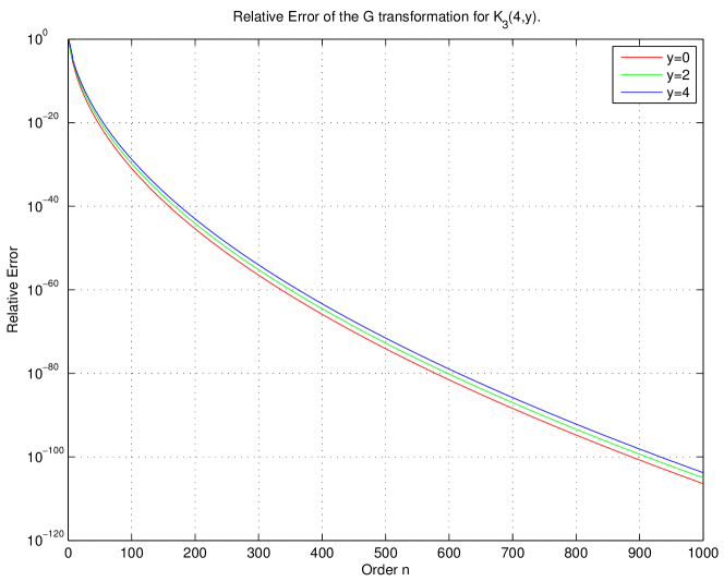
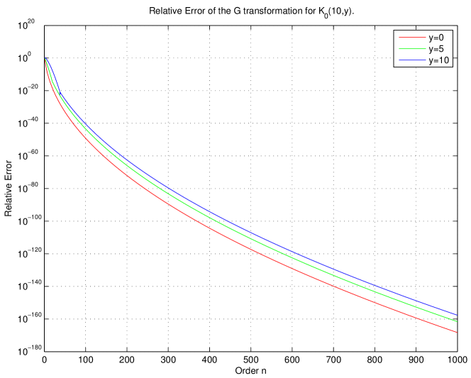
In Figures 1 and 2, the relative error of the transformation is shown for several different values of , , and . This figure shows the excellent stability and convergence properties of the improved algorithm that come with the use of the stable four-term recurrence relation.
4 Conclusion
We improve an existing algorithm for incomplete Bessel functions based on the transformation [15] by developing a recurrence relation the numerator sequence and the denominator sequence whose ratio form the sequence of approximations. By finding this recurrence relation, we reduce the complexity from to . We plot relative error showing that the algorithm is capable of extremely high accuracy for incomplete Bessel functions. The stability and convergence appear to be remarkable.
References
- [1] D.S. Jones. Incomplete Bessel functions. i. Proceedings of the Edinburgh Mathematical Society, 50:173–183, 2007.
- [2] D.S. Jones. Incomplete Bessel functions. II. asymptotic expansions for large argument. Proceedings of the Edinburgh Mathematical Society, 50:711–723, 2007.
- [3] M.S. Hantush and C.E. Jacob. Non-steady radial flow in an infinite leaky aquifer. Trans. Amer. Geophys. Union., 36:95–100, 1955.
- [4] F.E. Harris. New approach to calculation of the leaky aquifer function. Int. J. Quantum Chem., 63:913–916, 1997.
- [5] F.E. Harris. More about the leaky aquifer function. Int. J. Quantum Chem., 70:623–626, 1998.
- [6] F.E. Harris. On Kryachko’s formula for the leaky aquifer function. Int. J. Quantum Chem., 81:332–334, 2001.
- [7] B. Hunt. Calculation of the leaky aquifer function. J. Hydrol., 33:179–183, 1977.
- [8] E.S. Kryachko. Explicit expression for the leaky aquifer function. Int. J. Quantum Chem., 78:303–305, 2000.
- [9] F.E. Harris and J.G. Fripiat. Methods for incomplete Bessel evaluation. J. Comp. Appl. Math., 109:1728–1740, 2009.
- [10] M.M. Agrest and M.S. Maksimov. Theory of incomplete cylinder functions and their applications. Springer, Philadelphia, 1971.
- [11] L. Lewin. The near field of a locally illuminated diffracting edge. IEEE Trans. Antennas Propagat., AP19:134–136, 1971.
- [12] D.C. Chang and R.J. Fisher. A unified theory on radiation of a vertical electric dipole above a dissipative earth. Radio Sci., 9:1129–1138, 1974.
- [13] S.L. Dvorak. Applications for incomplete Lipschitz-Hankel integrals in electromagnetics. IEEE Antennas Propagat. Mag., 36:26–32, 1994.
- [14] M.M. Mechaik and S.L. Dvorak. Exact closed form field expressions for a semiinfinite traveling-wave current filament in homogeneous space. J. Electromagn. Waves Appl., 8:1563–1584, 1994.
- [15] R.M. Slevinsky and H. Safouhi. A recursive algorithm for the transformation and accurate computation of incomplete Bessel functions. App. Num. Math., 60:1411–1417, 2010.
- [16] P. Gaudreau, R.M. Slevinsky, and H. Safouhi. Computation of tail probability distributions via extrapolation methods and connection with rational and Padé approximants. SIAM J. Sci. Comput., 34:B65–B85, 2012.
- [17] D. Scott, T. Tran, R.M. Slevinsky, and H. Safouhi. The incomplete bessel K function in R Package DistributionUtils. http://cran.r-project.org/web/packages/DistributionUtils/, 2012.
- [18] R.M. Slevinsky and H. Safouhi. Useful properties of the coefficients of the slevinsky-safouhi formula for differentiation. Numerical Algorithm, 66:457–477, 2014.
- [19] D.D. Creal. Exact likelihood inference for autoregressive gamma stochastic volatility models. Research Seminar, pages 1–35, 2012.
- [20] D.D. Creal. A class of non-gaussian state space models with exact likelihood inference: Appendix. Working Paper, pages 1–28, 2013.
- [21] F. Nestler, M. Pippig, and D. Potts. Fast ewald summation based on nfft with mixed periodicity. Working Paper, pages 1–38, 2013.
- [22] F.E. Harris. Incomplete Bessel, generalized incomplete gamma, or leaky aquifer functions. J. Comp. Appl. Math., 215:260–269, 2008.
- [23] H.L. Gray and S. Wang. A new method for approximating improper integrals. SIAM J. Numer. Anal., 29:271–283, 1992.
- [24] H.L. Gray and T.A. Atchison. Nonlinear transformation related to the evaluation of improper integrals. I. SIAM J. Numer. Anal., 4:363–371, 1967.
- [25] H.L. Gray, T.A. Atchison, and G.V. McWilliams. Higher order -transformations. SIAM J. Numer. Anal., 8:365–381, 1971.
- [26] D.C. Joyce. Survey of extrapolation processes in numerical analysis. SIAM Rev., 13:435–490, 1971.
- [27] R.M. Slevinsky and H. Safouhi. New formulae for higher order derivatives and applications. J. Comput. App. Math., 233:405–419, 2009.
- [28] D. Levin and A. Sidi. Two new classes of non-linear transformations for accelerating the convergence of infinite integrals and series. Appl. Math. Comput., 9:175–215, 1981.