A robust and efficient method for estimating enzyme complex abundance and metabolic flux from expression data
Abstract
A major theme in constraint-based modeling is unifying experimental data, such as biochemical information about the reactions that can occur in a system or the composition and localization of enzyme complexes, with high-throughput data including expression data, metabolomics, or DNA sequencing. The desired result is to increase predictive capability and improve our understanding of metabolism. The approach typically employed when only gene (or protein) intensities are available is the creation of tissue-specific models, which reduces the available reactions in an organism model, and does not provide an objective function for the estimation of fluxes. We develop a method, flux assignment with LAD (least absolute deviation) convex objectives and normalization (FALCON), that employs metabolic network reconstructions along with expression data to estimate fluxes. In order to use such a method, accurate measures of enzyme complex abundance are needed, so we first present an algorithm that addresses quantification of complex abundance. Our extensions to prior techniques include the capability to work with large models and significantly improved run-time performance even for smaller models, an improved analysis of enzyme complex formation, the ability to handle large enzyme complex rules that may incorporate multiple isoforms, and either maintained or significantly improved correlation with experimentally measured fluxes. FALCON has been implemented in MATLAB and ATS, and can be downloaded from: https://github.com/bbarker/FALCON. ATS is not required to compile the software, as intermediate C source code is available. FALCON requires use of the COBRA Toolbox, also implemented in MATLAB.
1 Introduction
FBA (flux balance analysis) is the oldest, simplest, and perhaps most widely used linear constraint-based metabolic modeling approach [1, 2]. FBA has become extremely popular, in part, due to its simplicity in calculating reasonably accurate microbial fluxes or growth rates (e.g. Schuetz et al. 3, Fong and Palsson 4); for many microbes, a simple synthetic environment where all chemical species are known suffices to allow proliferation, giving fairly complete constraints on model inputs. Additionally, it has been found that their biological objectives can be largely expressed as linear objectives of fluxes, such as maximization of biomass [3]. Neither of these assumptions necessarily hold for mammalian cells growing in vitro or in vivo, and in particular the environment is far more complex for mammalian cell cultures, which have to undergo gradual metabolic adaptation via titration to grow on synthetic media [5]. Recently, there have been many efforts to incorporate both absolute and differential expression data into metabolic models [6]. The minimization of metabolic adjustment (MoMA; Segrè et al. 7) algorithm is the simplest metabolic flux fitting algorithm, and it can be extended in order to allow the use of absolute expression data for the estimation of flux [8], which is the approach taken in this study. A different approach for using expression in COBRA, also very simple, is E-flux, which simply uses some function of expression (chosen at the researcher’s discretion; typically a constant multiplier of expression) as flux constraints [9]. Despite this surprising simplicity, the method has found many successful applications, but the user-chosen parameter and use of expression as hard constraints is, in our opinion, a detraction, and others have had better results taking an approach similar to Lee et al. 8 [10].
The MoMA method, framed as a constrained least-squares optimization problem, is typically employed to calculate the flux vector of an in silico organism after a mutation by minimizing the distance between the wild-type flux and the mutant flux. The biological intuition is that the organism has not had time to adapt to the restricted metabolic capacity and will maintain a similar flux to the wild-type (WT) except where the perturbations due to the mutation dictate necessary alterations in fluxes [11]. Suppose is the WT flux vector obtained by an optimization procedure such as FBA, empirical measurements, or a combination of these. For an undetermined flux vector in a model with reactions the MoMA objective can be expressed as
| (1) |
subject to the stoichiometric constraints where and is the stoichiometric matrix (rows correspond to metabolites, columns to reactions, and entries to stoichiometric coefficients). Constant bounds on fluxes are often present, such as substrate uptake limits, or experimental estimates, so we write these as the constraints . The objective may be equivalently expressed in the canonical quadratic programming (QP) vector form as . This assumes that each is measured, but it is also possible and sometimes even more useful to employ this objective when only a subset of the are measured (if is not measured for some , then we omit from the objective). In metabolomics, for instance, it is always the case in experiments with labeled isotope tracers that only a relatively small subset of all fluxes are able to be estimated with metabolic flux analysis (MFA; Shestov et al. 1). Combining MoMA with MFA provides a technique to potentially estimate other fluxes in the network.
A variant of MoMA exists that minimizes the absolute value of the difference between and for all known . To our knowledge, the following linear program is the simplest version of linear MoMA, which assumes the existence of a constant flux vector :
|
(2) |
The are just the distances from a priori fluxes to their corresponding fitted fluxes. Linear MoMA has the advantage that it is not biased towards penalizing large magnitude fluxes or under-penalizing fluxes that are less than one [12, 11]. Additionally, linear programs are often amenable to more alterations that maintain convexity than a quadratic program and tend to have fewer variables take on small values, and it is much easier to interpret the importance of a zero than a small value [12].
We wish to apply MoMA to expression data rather than flux data, but there are two primary problems that must be tackled. First, we must quantify enzyme complex abundance as accurately as possible given the gene expression data. Although there is not a one-to-one correspondence between reactions and enzyme complexes, the correspondence is much closer than that between individual genes and metabolic reactions. In the first part of this work, we employ an algorithm that can account for enzyme complex formation and thus quantify enzyme complex abundance. Second, we must fit real-valued variables (fluxes) to non-negative data (expression), which is challenging to do efficiently. To accomplish this, we build on the original MoMA objective, which must be altered in several ways (also discussed in Lee et al. 8, which lays the groundwork for the current method). We develop automatic scaling of expression values so that they are comparable to flux units obtained in the optimization routine. This can be an advantage over the prior method as it no longer requires the manual choice of a flux and complex abundance pair with a ratio that is assumed to be representative of every such pair in the system. Related to this, we also implement the sharing of enzyme complex abundance between the reactions that the complex catalyzes, rather than assuming there is no competition between reactions catalyzed by the same complex. Reaction direction assignment enables comparison of fluxes and expression by changing fluxes to non-negative values. We show that batch assignment, rather than serial assignment [8] of reaction direction can greatly improve time efficiency while maintaining or slightly improving correlations with experimental fluxes. In addition to several of the methods described so far, we also included in our comparison two methods for tissue-specific modeling. In GIMME, the authors remove reactions whose associated gene expression is below some threshold, then add reactions that preclude some user-defined required metabolic functionalities in an FBA objective back into the model, and finally use FBA again to obtain fluxes [13]. The other tissue-specific method we compared with is iMAT, which employs a mixed integer linear programming (MILP) problem to maximize the number of reactions whose activity corresponds to their expression state (again using thresholds, but this time, there are low, medium, and highly expressed genes, and only the lowly and highly expressed genes are included in the objective) all while subject to typical constraints found in FBA [14].
Finally, we employ several sensitivity analyses and performance benchmarks so that users of the FALCON method and related methods may have a better understanding of what to expect in practice.
2 Methods
Most genome-scale models have attached Boolean (sans negation) gene rules to aid in determining whether or not a gene deletion will completely disable a reaction. These are typically called GPR (gene-protein-reaction) rules and are a requirement for FALCON; their validity, like the stoichiometric matrix, is important for generating accurate predictions. Also important are the assumptions and limitations for the process of mapping expression data to complexes so that a scaled enzyme complex abundance (hereafter referred to as complex abundance) can be estimated. We address these in the next section and have attached a flow chart to illustrate the overall process of mapping expression of individual genes to enzyme complexes within the greater context of flux estimation (Figure 1). We employ an algorithm for this step—finding the minimum disjunction—for estimating complex abundance as efficiently and as accurately as possible given the assumptions (Section 8).
Consideration of constraint availability, such as assumed reaction directions and nutrient availability, is crucial in this type of analysis. In order to work with two sets of constraints with significantly different sizes in yeast, we wrote the MATLAB function removeEnzymeIrrevs to find all enzymatic reactions in a model that are annotated as reversible but are constrained to operate in one direction only. This is not something a researcher would normally want to do since constraints should generally act to improve modeling predictions, but we are interested to see how their removal influences model predictions and solution robustness.
The function useYN5irrevs copies the irreversible annotations found in Yeast 5.21 [8] to a newer yeast model, but could in principle be used for any two models; by default, this script is coded to first call removeEnzymeIrrevs on both models before copying irreversible annotations. Application of these scripts removes 853 constraints in Yeast 5.21 and 1,723 constraints in Yeast 7. Despite the significant relaxation in constraints, since nutrient uptake constraints are unaffected, FBA only predicts a 1.28% increase in growth rate in the minimally constrained Yeast 7 model. However, in FALCON, we are no longer optimizing a sink reaction like biomass, and this relaxation in internal constraints proves to be more important. Constraint sets for Human Recon 2 are described in Figure 8.
2.1 Estimating enzyme complex abundance
Given the diversity and availability of genome-scale expression datasets, either as microarray or more recently RNA-Seq, it could be useful to gauge the number of enzyme complexes present in a cell. A recent study found that only 11% of annotated Drosophila protein complexes have subunits that are co-expressed [15], so it cannot be assumed that any given protein subunit level represents the actual complex abundance. We formalize a model for enzyme complex formation based on GPR rules that are frequently available in genome-scale annotations.
The original expression to complex abundance mapping procedure [8] performed a direct evaluation of GPR rule expression values—replacing gene names with their expression values, ANDs with minimums, and ORs with sums, without altering the Boolean expression of the GPR rule in any way. Below we illustrate a problem that can occur with this mapping where some genes’ expression levels may be counted more than once.
The are different reaction rules and the are the corresponding estimated complex abundance levels. Lower case letters are shorthand for the expression level of the corresponding gene ID in uppercase; for example, , where is the expression of gene A.
|
(3) |
Supposing A is the minimum, then if we just evaluate directly (a rule in disjunctive normal form, or DNF), A will be counted twice. Rules with sub-expressions in DNF are frequently encountered in practice, but directly evaluating them can lead to erroneous quantification.
Another possibility is partitioning expression among multiple occurrences of a gene in a rule. For instance, in above, we could evaluate it as = min() + min() to account for the repeated use of . However, other potential issues aside, we can see that this can cause problems rather quickly. For instance, suppose and ; then min(,) appears to be correct, not min() + min() = . From this example, we can see that conversion to conjunctive normal form (CNF; Russell and Norvig 16), as in appears to be a promising prerequisite for evaluation.
2.2 The min-disjunction algorithm estimates enzyme complex abundance
In Section 8, we show that converting a rule to CNF is a sound method to aid in the estimation of enzyme complex abundance. The minimum disjunction algorithm is essentially just the standard CNF conversion algorithm [16], with the implementation caveat that a gene that is in disjunction with itself should be reduced to a literal. We’ve found that this makes the CNF conversion algorithm tractable for all rules and prevents double counting of gene expression. Conversion to CNF and selection of the minimum disjunction also removes redundant genes from the complex (e.g. holoenzymes; see Assumption 8). Biologically, selecting the minimum disjunction effectively finds the rate-limiting component of enzyme-complex formation. After conversion to CNF, the minimum disjunction algorithm substitutes gene-expression values as described in Lee et al. 8 and evaluates the resulting arithmetic expression. Another new feature of our approach is the handling of missing gene data. If expression is not measured for a gene in a GPR rule, the rule is modified so that the missing gene is no longer part of the Boolean expression. For instance, if data is not measured for gene B in [A and (B or C)] then the rule would become [A and C]. This prevents penalization of the rule’s expression value in the case that the missing gene was part of a conjunction, and it also assumes there was no additional expression from the missing gene if it is in a disjunction.
Although conversion to CNF may be intractable for some expressions [16], we tested our implementation of the algorithm on three of the most well-curated models which contain some of the most complex GPR rules available. These models are for E. coli [17], yeast [18], and human [19]. In all cases, the rules were converted to CNF in less than half a second, which is far less than the typical flux fitting running time from Algorithm 3.1.
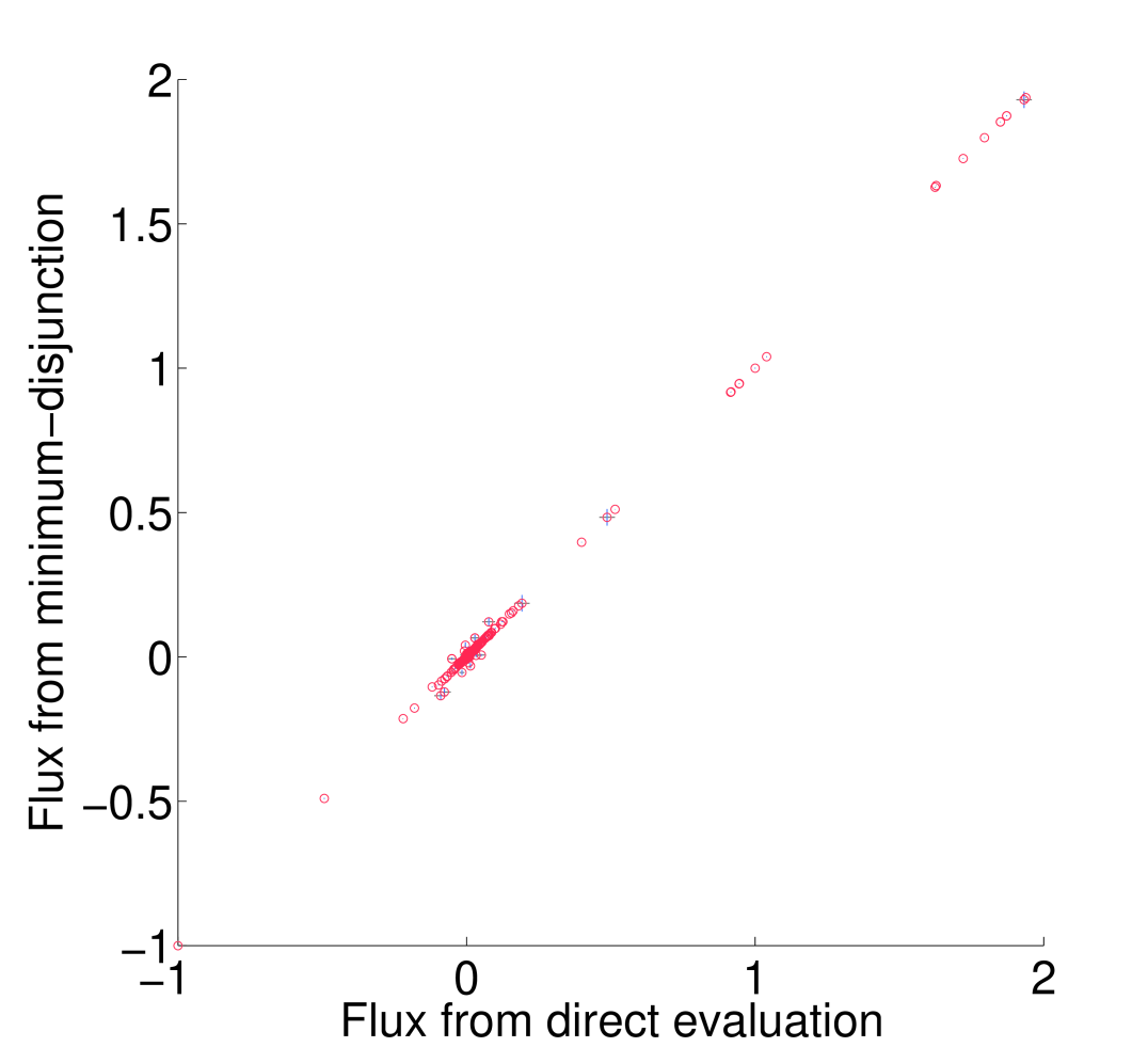
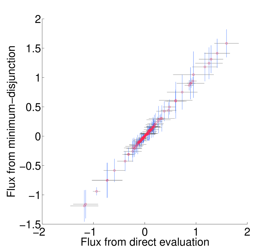
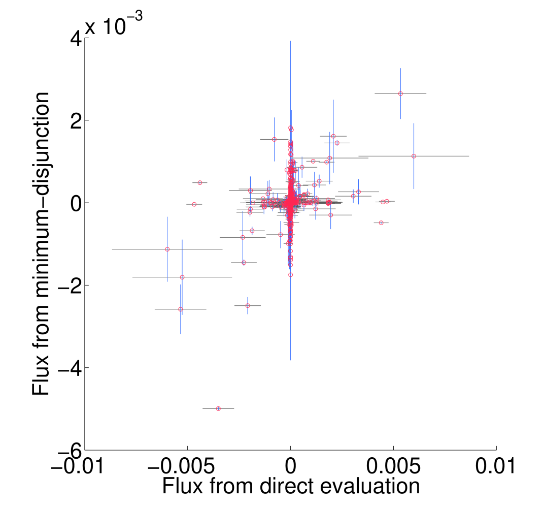
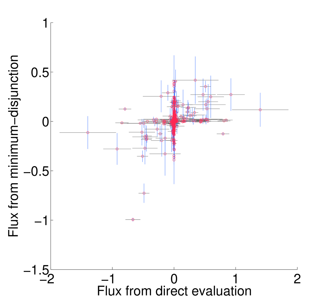
Using the minimum disjunction method results in several differences from direct substitution and evaluation in yeast GPR rules. When data completely covers the genes in the model (e.g. Lee et al. 8), complex abundance tends to have few differences in yeast regardless of the evaluation method (25 rules; 1.08% of all rules for Yeast 7). This number goes up significantly in Human Recon 2 [19] due to more complex GPR rules (935 rules; 22% of all rules). For the human model, we could not find any data set that covered every gene, so instead random expression data roughly matching a power law was used to generate this statistic. If we use proteomics data for yeast and human models, the algorithmic variation in how missing gene data is handled causes some additional increase in differences [20, 21]. For proteomics, in the Yeast 7 model 205 rules (8.87% of all rules) differed, and in Human Recon 2, 1002 rules (23.57% of all rules) differed. We can see that for yeast, the changes in flux attributed to enzyme abundance evaluation can be relatively small for data with 100% gene coverage, but can be significant in Human (Figure 5).
3 The FALCON algorithm
Prior work that served as an inspiration for this method used Flux Variability Analysis (FVA) to determine reaction direction [8]. Briefly, this involves two FBA simulations per reaction catalyzed by an enzyme, and as the algorithm is iterative, this global procedure may be run several times before converging to a flux vector. We removed FVA to mitigate some of the cost, and instead assign flux direction in batch; while it is possible that the objective value may decrease in subsequent iterations of the algorithm, this is not an issue since the objective function is changed at each iteration to include more irreversible fluxes. The objective value of a function with more fluxes should supersede the importance of one with fewer fluxes, as the functions are not the same and thus not directly comparable, and we wish to include as many data points in the fitting as possible.
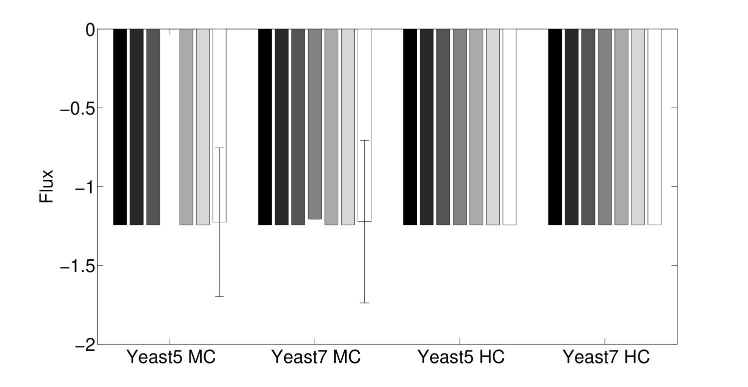
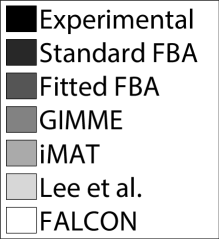
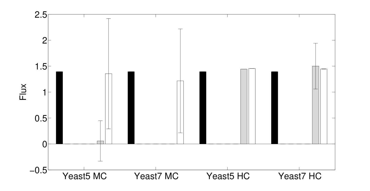
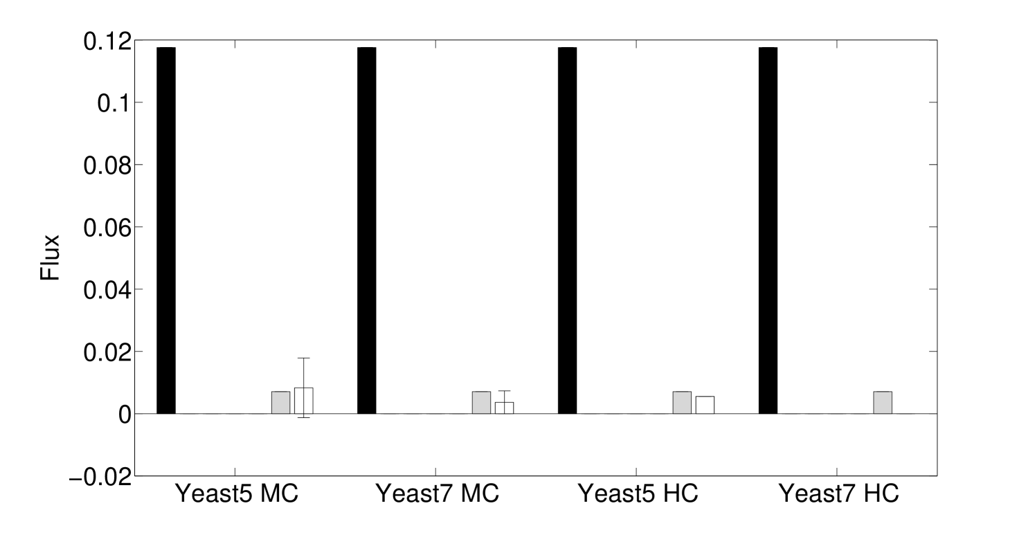
One major advance in our method is the consideration of enzyme complexes sharing multiple reactions, which we call reaction groups. This is done by partitioning an enzyme complex’s abundance across its reactions by including all reactions associated to the complex in the same constraint. Both minimally and highly constrained models (Section 4.2) show some fluxes with significant differences depending on the use of group information, particularly in the minimally constrained model (Figure 2). We now discuss the algorithm in detail, including several other important features, including automatic scaling of expression.
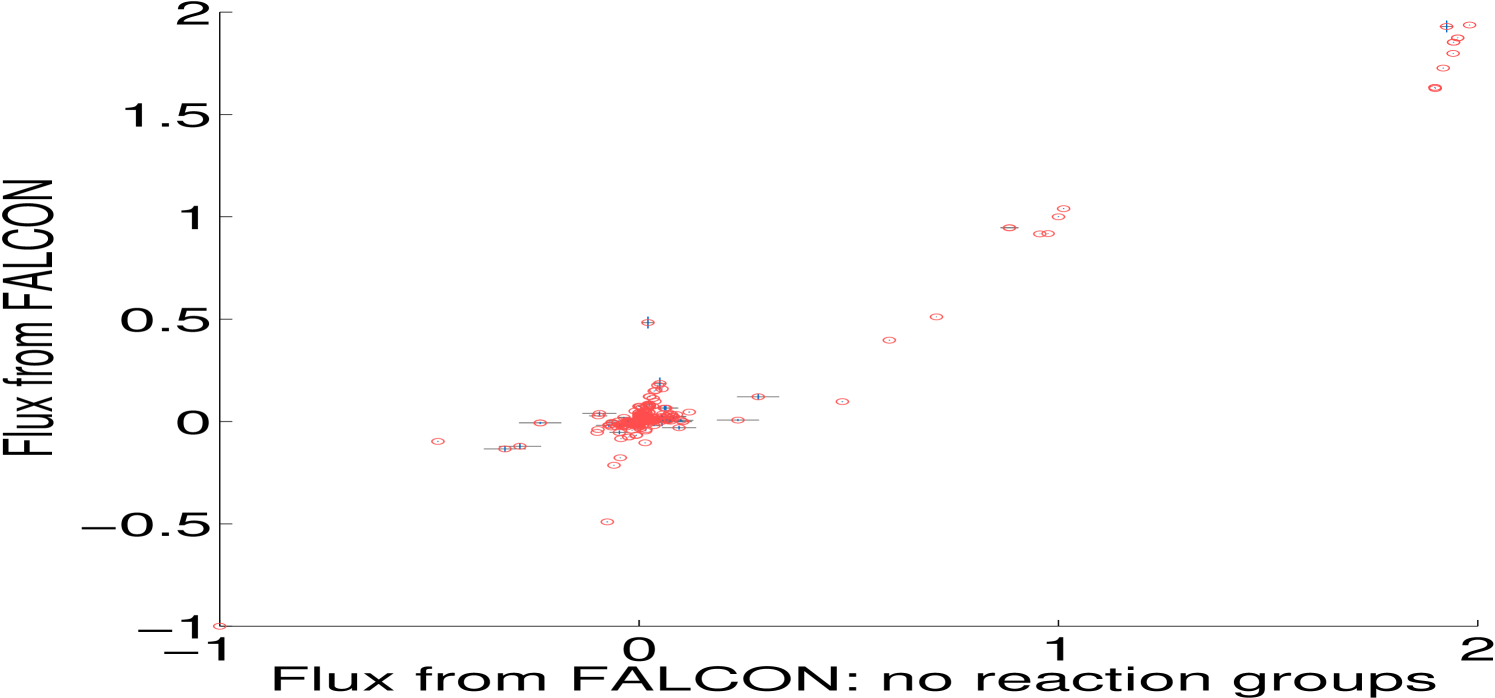
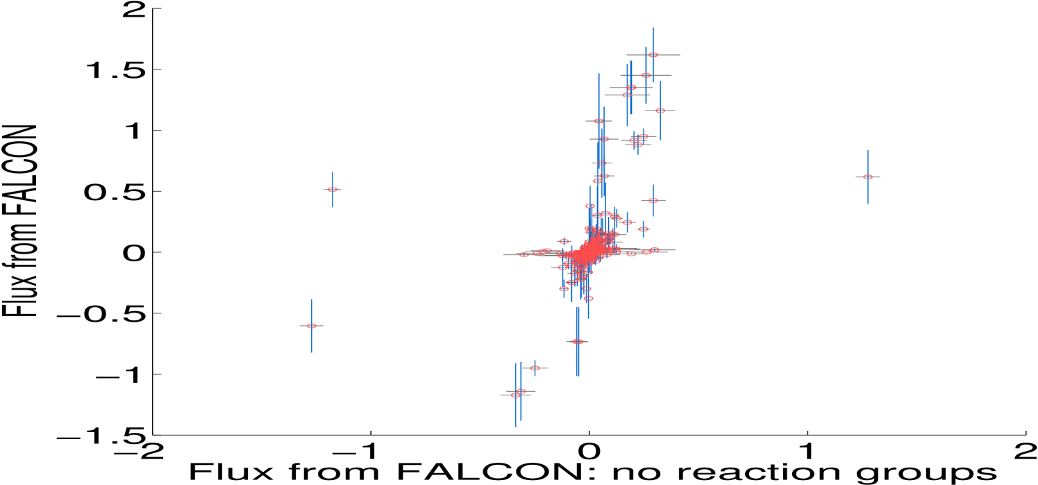
To make working with irreversible fluxes simpler, we convert the model to an irreversible model, where each reversible flux in the original model is split into a forward and a backward reaction that take strictly positive values: and . We also account for enzyme complexes catalyzing multiple reactions by including all reactions with identical GPR rules in the same residual constraint; indexed sets of reactions are denoted and their corresponding estimated enzyme abundance is . Figure 2 shows the difference in Algorithm 3.1 when we do not use reaction group information. The standard deviation of enzyme abundance, , is an optional weighting of uncertainty in biological or technical replicates.
We employ a normalization variable in the problem’s objective and flux-fitting constraints to find the most agreeable scaling of expression data. The linear fractional program shown below can be converted to a linear program by the Charnes-Cooper transformation [12]. To avoid the need for fixing any specific flux, which may introduce bias, we introduce the bound . This guarantees that the optimization problem will yield a non-zero flux vector. As an example of how this can be beneficial, this means we do not need to measure any fluxes or assume a flux is fixed to achieve good results; though this does not downplay the value of obtaining experimentally-based constraints on flux when available (Figure 6).
The actual value of is not very important due to the scaling introduced by , and we include a conservatively small value that should work with any reasonable model. However, for numeric reasons, it may be best if a user chooses to specify a value appropriate for the model. Similarly, if any fluxes are known or assumed to be non-zero, this constraint becomes unnecessary. To keep track of how many reactions are irreversible in the current and prior iteration, we use the variables and . The algorithm terminates when no reactions are constrained to be exclusively forward or backward after an iteration.
Algorithm 3.1 and the method in Lee et al. 8 are both non-deterministic. In the first case, Algorithm 3.1 solves an LP during each iteration, and subsequent iterations depend on the LP solution, so that alternative optima may affect the outcome. In the latter case, alternative optima of individual LPs is not an issue, but the order in which reactions assigned to be irreversible can lead to alternative solutions. However, we found that the variation due to this stochasticity is typically relatively minor, particularly in cases where the model is more heavily constrained (Figs. 5 and 6).
4 Results and Discussion
4.1 Performance benchmarks
Using the same yeast exometabolic and expression data employed for benchmarking in the antecedent study [8] that included an updated version of the Yeast 5 model [22] and the latest yeast model [18], we find that our algorithm has significant improvements in time efficiency while maintaining correlation with experimental fluxes, and is much faster than any similarly performing method (Table 1; Figure 6). Timing for the human model also improved in FALCON; in a model with medium constraints and exometabolic directionality constraints, FALCON completed on average in 3.6 m and the method from Lee et al. 8 in 1.04 h. Furthermore, when we remove many bounds constraining the direction of enzymatic reactions that aren’t explicitly annotated as being irreversible in prior work [8], we find that our formulation of the approach seems to be more robust than other methods.
| (a) | Max. | Model | Experimental | Standard FBA | Fitted FBA | GIMME | iMAT | Lee et al. | FALCON |
|---|---|---|---|---|---|---|---|---|---|
| 75 % | Yeast 5 MC | 1 | 0.66 | 0.66 | NaN | 0.57 | 0.64 | 1 | |
| 75 % | Yeast 7 MC | 1 | 0.66 | 0.66 | 0.68 | 0.66 | 0.66 | 0.98 | |
| 75 % | Yeast 5 HC | 1 | 0.73 | 0.78 | 0.75 | 0.66 | 0.98 | 0.99 | |
| Pearson’s r | 75 % | Yeast 7 HC | 1 | 0.70 | 0.70 | 0.80 | 0.66 | 0.98 | 0.99 |
| 85 % | Yeast 7 MC | 1 | 0.62 | 0.62 | 0.65 | 0.62 | 0.62 | 0.97 | |
| 85 % | Yeast 5 HC | 1 | 0.88 | 0.89 | 0.9 | 0.81 | 0.99 | 0.99 | |
| 85 % | Yeast 7 HC | 1 | 0.67 | 0.67 | 0.87 | 0.62 | 0.98 | 0.98 |
| (b) | Max. | Model | Experimental | Standard FBA | Fitted FBA | GIMME | iMAT | Lee et al. | FALCON |
| 75 % | Yeast 5 MC | 0 | 0.9 | 470 | 0.81 | 50 | 110 | 1.8 | |
| 75 % | Yeast 7 MC | 0 | 1.9 | 3,100 | 2.1 | 12,000 | 600 | 5.6 | |
| 75 % | Yeast 5 HC | 0 | 0.12 | 110 | 0.18 | 1.4 | 15 | 0.27 | |
| Time (s) | 75 % | Yeast 7 HC | 0 | 0.72 | 940 | 1.7 | 240 | 670 | 5.5 |
| 85 % | Yeast 7 MC | 0 | 2.3 | 3,100 | 3.8 | 14,000 | 610 | 4.6 | |
| 85 % | Yeast 5 HC | 0 | 0.12 | 110 | 0.18 | 2.5 | 15 | 0.22 | |
| 85 % | Yeast 7 HC | 0 | 0.70 | 110 | 2.5 | 100 | 530 | 5.9 |
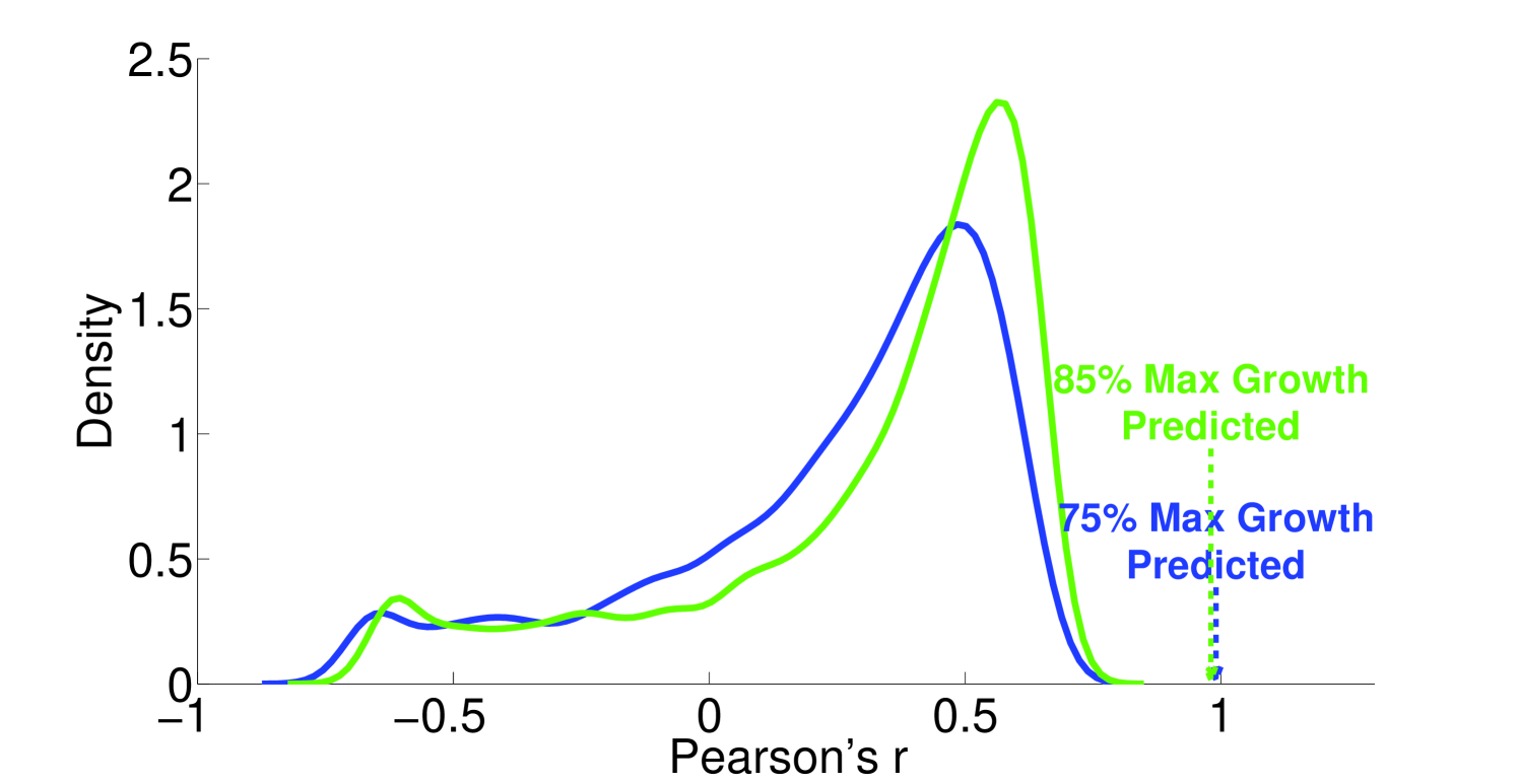
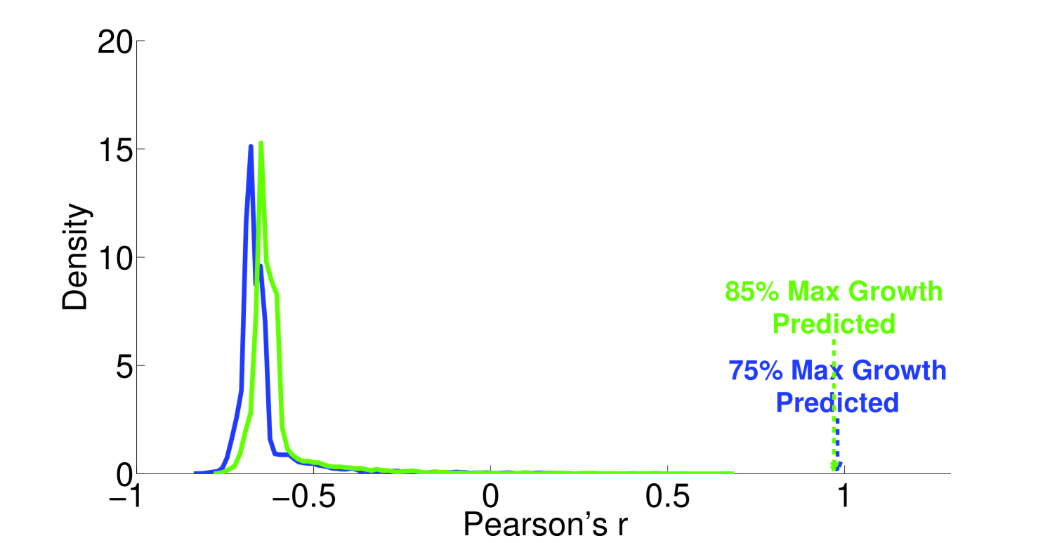
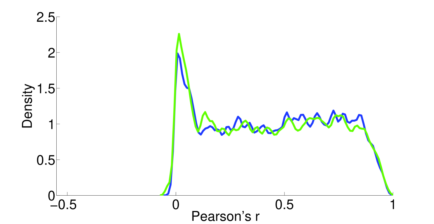
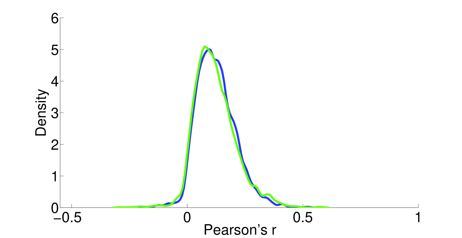
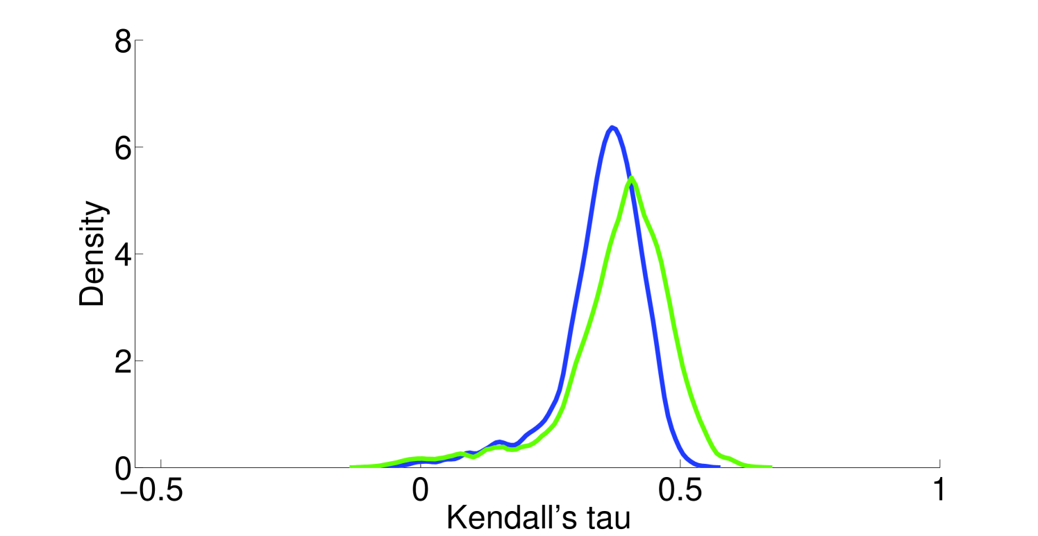
We see that the predictive ability of the algorithm does not appear to be an artifact; when FALCON is run on permuted expression data, it doesn’t do as well as the actual expression vector (Figure 3). The full-sized flux vectors estimated from permuted expression as a whole also does not correlate well with the flux vector estimated from the actual expression data, but we notice that the difference is visibly larger in the minimally constrained model compared to the highly constrained model (Figure 7). Rigidity in the highly constrained model appears to keep most permutations from achieving an extremely low Pearson correlation, likely due to forcing fluxes through the same major pathways, but a rank-based correlation still shows strong differences.
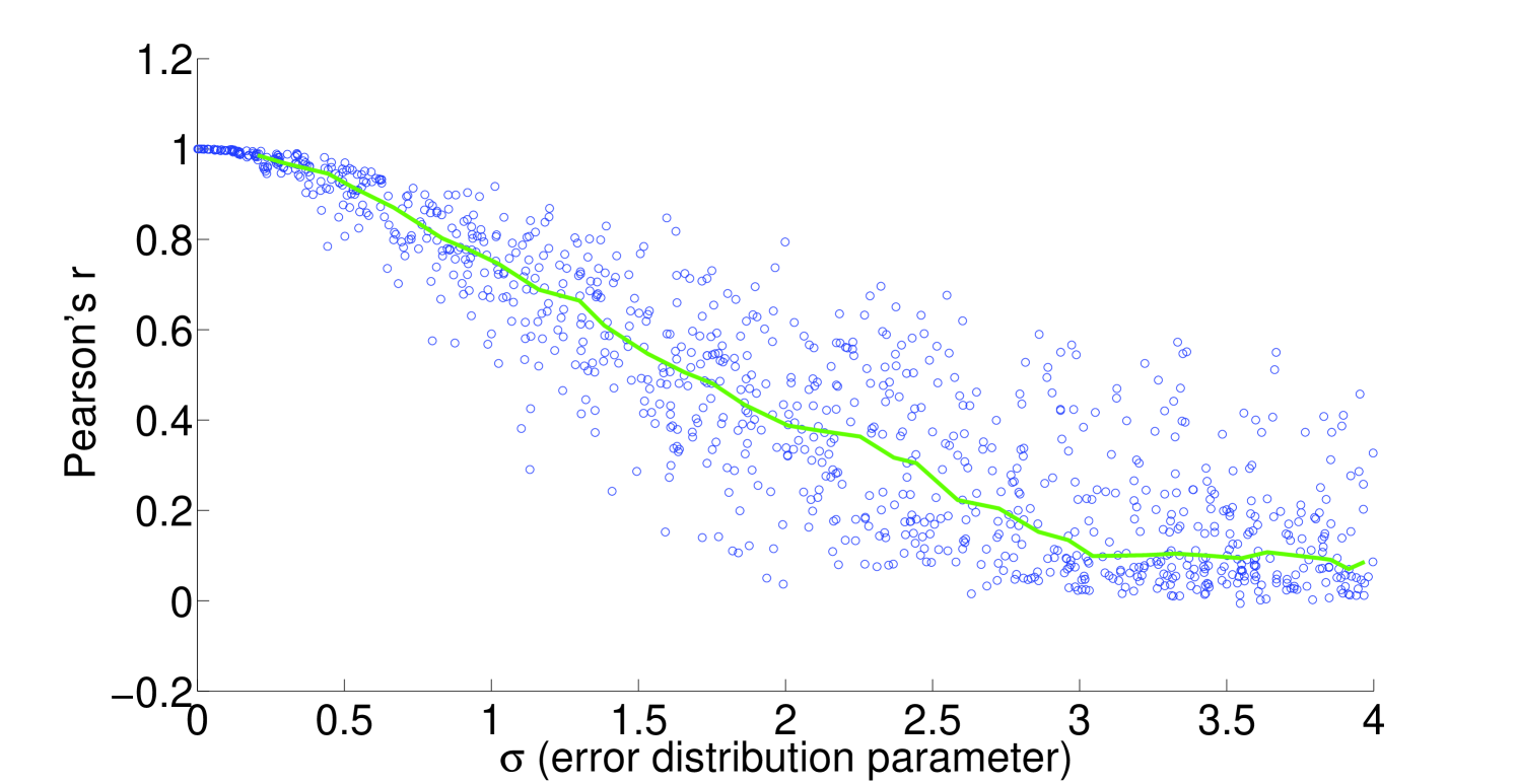
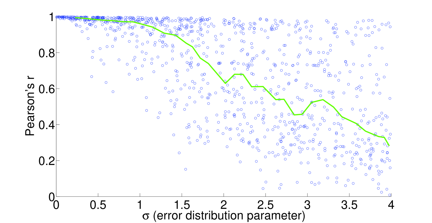
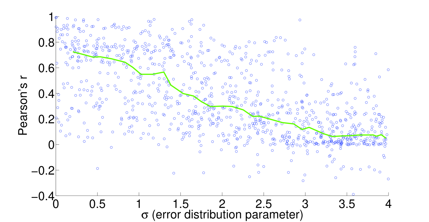
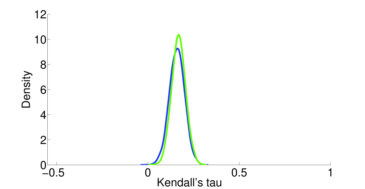
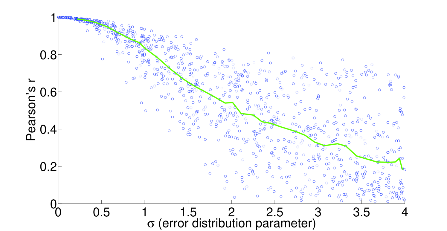
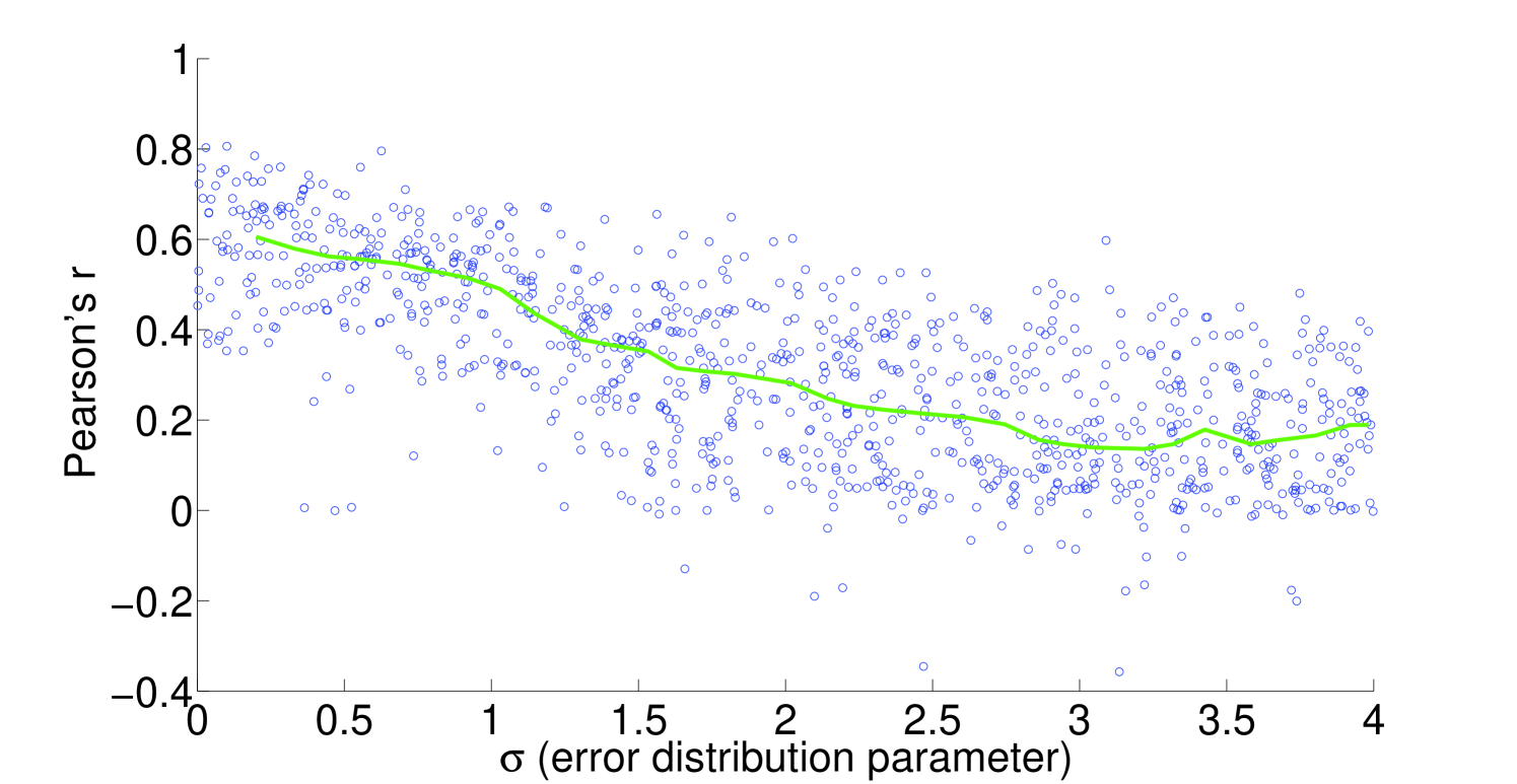
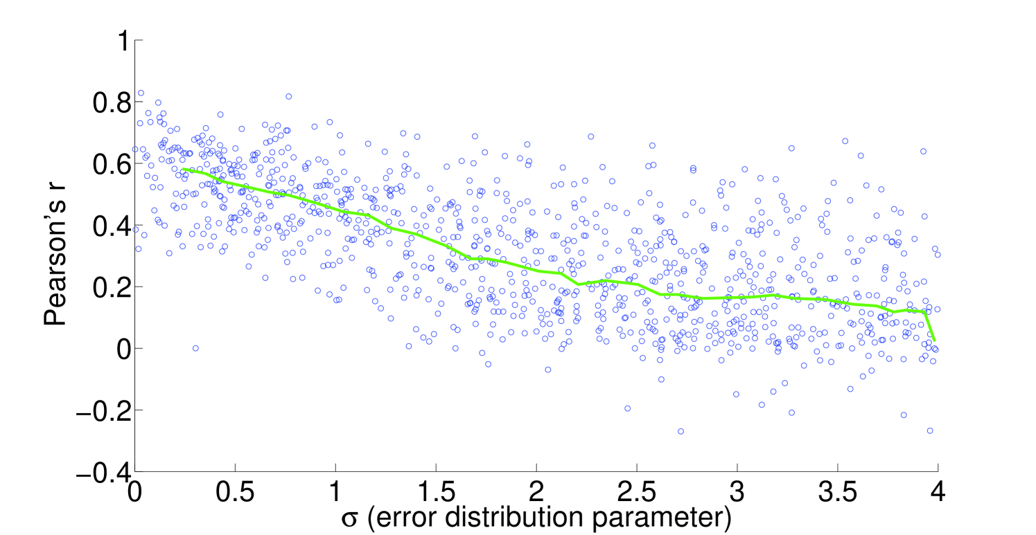
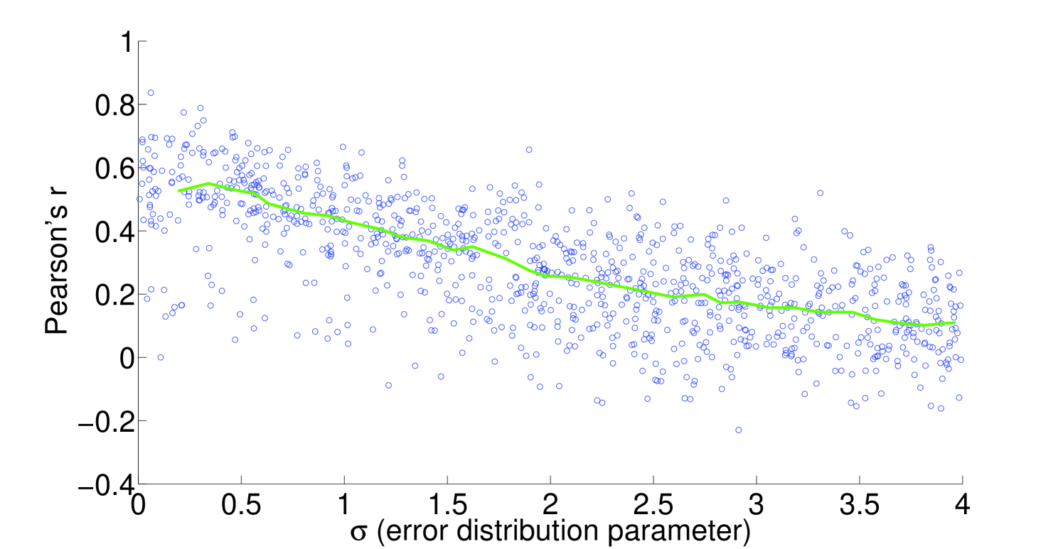
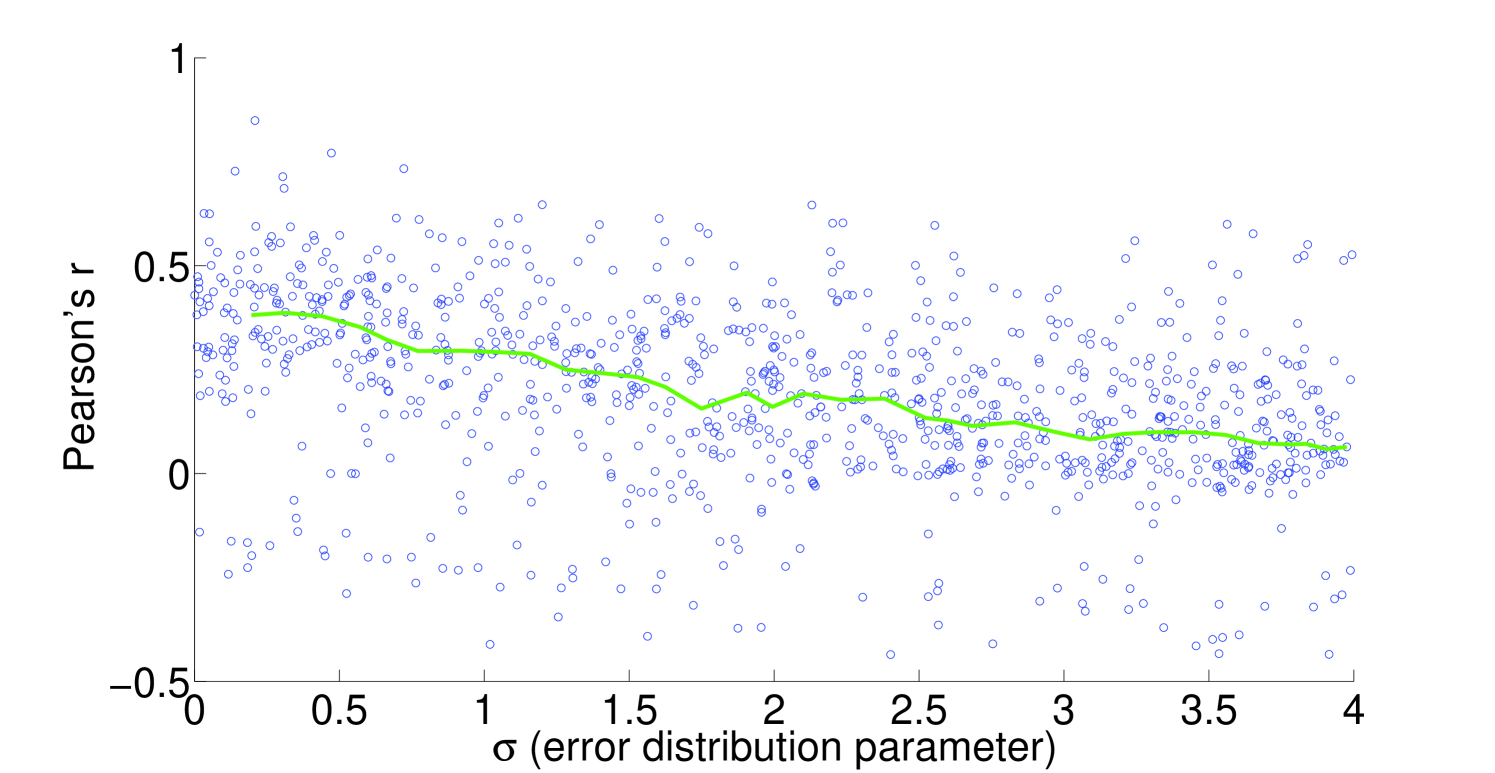
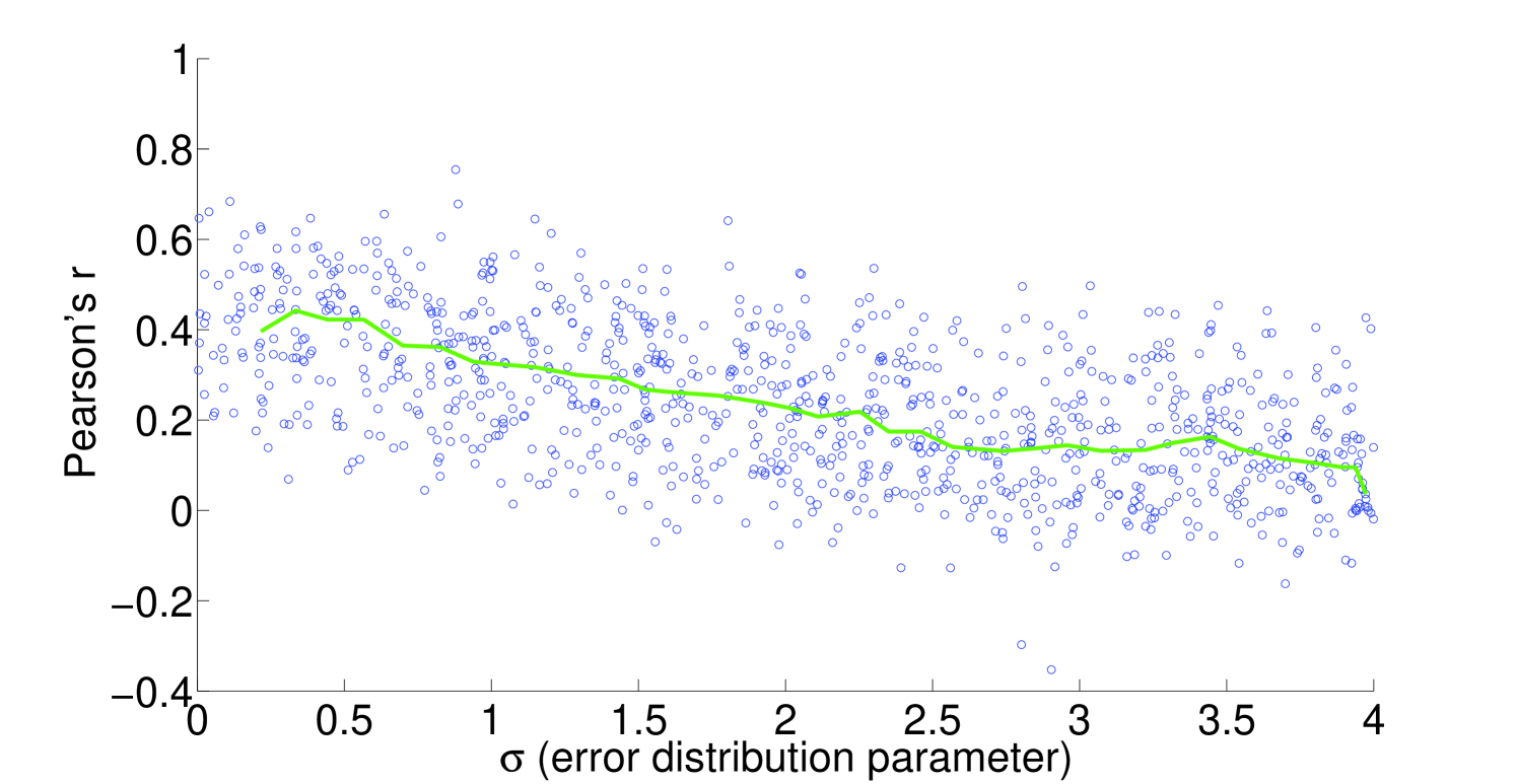
4.2 Sensitivity to expression noise
To understand the sensitivity of flux to expression, we multiply noise from multivariate log-normal distributions with the expression vector and see the effect on the estimated fluxes. For instance, correlation between two types of proteomics data yields a Pearson’s [21], corresponding to an expected and expected for flux in our most highly constrained human model (Figure 8). We find that enzymatic reaction directionality constraints influence the sensitivity of the model to expression perturbation (Figure 4). It is important to note that mere presence of the constraints does not help us determine the correct experimental fluxes when other classes of methods (e.g. FBA; Table 1) are used. Additionally, it is possible to obtain good predictions even without a heavily constrained model (Table 1).
With Human Recon 2, additional constraint sets supply some benefit, but even the most extreme constraint set does not compare to what is available in Yeast 7, which is also inherently constrained by the fact that yeast models will be smaller than comparable human models (Figure 8). For mammalian models, more sophisticated means of constraint, such as enzyme crowding constraints [23], or using FALCON in conjunction with tissue specific modeling tools, may prove highly beneficial.
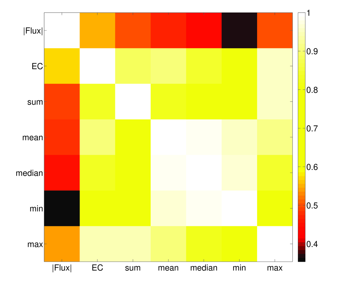
4.3 Flux estimates provides information beyond enzyme complex abundance
It is not an unreasonable hypothesis that fluxes would correlate well with their associated complex abundances. Indeed, the general principle needed for fitting fluxes to enzyme complex abundances is to assume the values would be correlated in the absence of other constraints (e.g. branch points that arise from the stoichiometry). More specifically, it should be the case that flux is proportional to enzyme complex abundance given ample availability of substrate, and that this proportionality constant does not vary too much between reactions. There are undoubtedly many exceptions to this rule, but it seems as though there may be some underlying evolutionary principles for it to work in this parsimonious fashion, as has been partly verified [24].
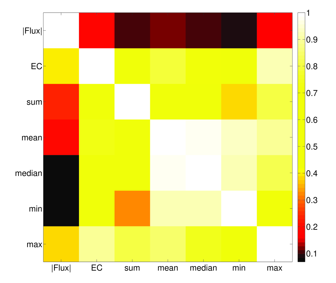
Aside from the obvious benefits of constraint-based methods also estimating fluxes for non-enzymatic reactions, and assigning a direction for reversible enzymatic reactions, we see that in general, our method does not predict a strong correlation between complex abundance and flux (Figure 9). Recently it has been shown that many fluxes are not under direct control of their associated enzyme expression level [25], which gives experimental support to the idea that a network-based approach, such as that presented in this paper, may be useful in understanding how fluxes may be constrained by expression data. Chubukov et al. 25 also note that enzymes may be overexpressed in some cases, either for robustness or because of noise in transcriptional regulation. This will not usually be a problem in FALCON, unless entire pathways are overexpressed, which would be unusual as it would represent a seemingly large energetic inefficiency.
The present work doesn’t attempt to use empirically obtained kinetic parameters to estimate , but this approach does not seem as promising in light of experimental evidence that many reactions in central carbon metabolism tend to operate well below [24]. Still, a better understanding of these phenomena may make it possible to improve flux estimation methods such as the one presented here, or more traditional forms of MFA [1] by incorporating enzyme complexation and kinetic information.
4.4 Increasing roles for GPR rules and complex abundance estimates
Still, complex abundance may have uses aside from being a first step in FALCON. The method presented here for complex abundance estimation can be used as a stand-alone method, as long as GPR rules from a metabolic reconstruction are present. For instance, it may not always be desirable to directly compute a flux. As an example, the relative abundance of enzyme complexes present in secretions from various biological tissues, such as milk or pancreatic secretions, may still be of interest even without any intracellular flux data. Perhaps more importantly, this approach to estimating relative complex levels can be employed with regulatory models such as PROM [26] or other regulatory network models that can estimate individual gene expression levels at time given the state of the model at a time .
GPR rules and stoichiometry may be inaccurate or incomplete in any given model. In fact, for the foreseeable future, this is a given. By using the GPR and not just the stoichiometry to estimate flux, it is possible that future work could make use of this framework to debug not just stoichiometry as some methods currently do (e.g. Reed et al. 27) , but also GPR rules. Hope for improved GPR rule annotation may come from many different avenues of current research. For instance, algorithms exist for reconstructing biological process information from large-scale datasets, and could be tuned to aid in the annotation of GPR rules [28]. Flexible metabolic reconstruction pipelines such as GLOBUS may also be extended to incorporate GPR rules into their output, and in so doing, extend this type of modeling to many non-model organisms [29]. Another limitation that relates to lack of biological information is that we always assume a one-to-one copy number for each gene in a complex. Once more information on enzyme complex structure and reaction mechanism becomes available, an extension to the current method could make use of this information. Even at the current level of structure, we think it is evident that GPR rules should undergo some form of standardization; Boolean rules without negation may not always capture the author’s intent for more complex purposes like flux fitting.
5 Conclusion
We have formalized and improved an existing method for estimating flux from expression data, as well as listing detailed assumptions in Table 2 that may prove useful in future work. Although we show that expression does not correlate well with flux, we are still essentially trying to fit fluxes to expression levels. The number of constraints present in metabolic models (even the minimally constrained models) prevents a good correlation between the two. However, as with all constraint-based models, constraints are only part of the problem in any largely underdetermined system. We show that gene expression can prove to be a valuable basis for forming an objective, as opposed to methods that only use expression to further constrain the model by creating tissue-specific or condition-specific models [9, 14, 13, 30].
For better curated models, the approach described immediately finds use for understanding metabolism, as well as being a scaffold to find problems for existing GPR rules, and more broadly the GPR formalism itself. The present results and avenues for future improvement show that there is much promise for using expression to estimate fluxes, and that it can already be a useful tool for performing flux estimation and analysis.
6 Acknowledgments
We thank Neil Swainston for his previous work on these research issues and many helpful discussions about considerations in various genome scale models of metabolism. We also thank Michael Stillman for general discussions about modeling and for reading the paper. Finally we thank Alex Shestov, Lei Huang, and Eli Bogart for many helpful discussions about metabolism.
BEB and YW are supported by the Tri-Institutional Training Program in Computational Biology and Medicine. BEB and ZG are thankful for support from NSF grant MCB-1243588. KS is grateful for the financial support of the EU FP7 project BioPreDyn (grant 289434). CRM acknowledges support from NSF Grant IOS-1127017. JWL thanks the NIH for support through grants R00 CA168997 and R01 AI110613.
7 Supporting figures
8 Assumptions for enzyme complex formation
In order to quantify enzyme complex formation (sometimes called enzyme complexation), the notion of an enzyme complex should be formalized. A protein complex typically refers to two or more physically associated polypeptide chains, which is sometimes called a quaternary structure. Since we are not exclusively dealing with multiprotein complexes, we refer to an enzyme complex as being one or more polypeptide chains that act together to carry out metabolic catalysis.
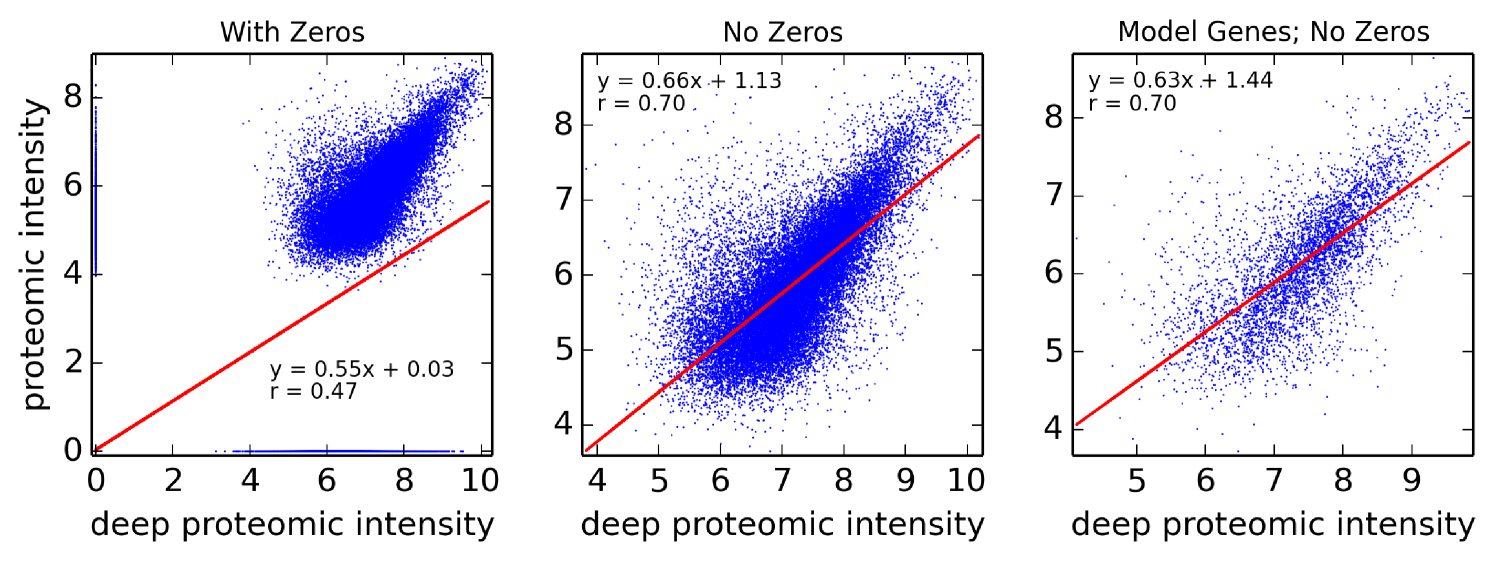
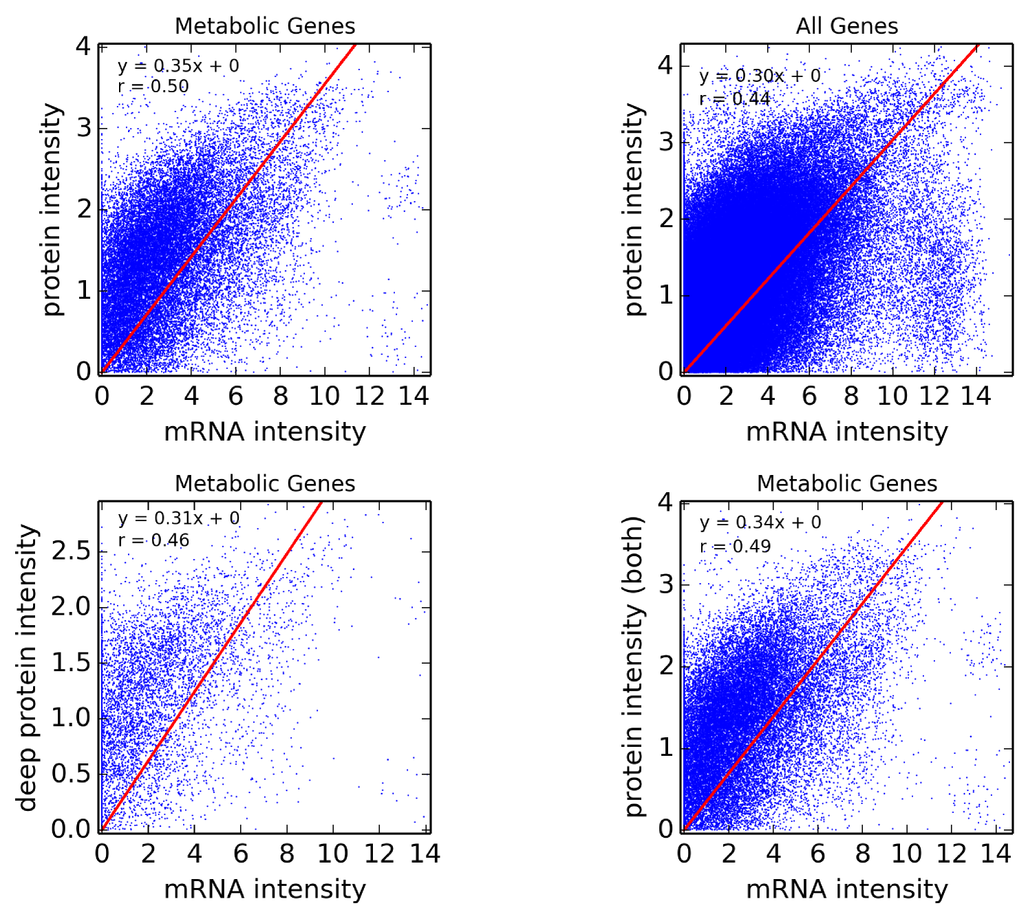
Assumption 1. A fundamental assumption that we need in order to guarantee an accurate estimate of (unitless) enzyme complex abundance are the availability of accurate measurements of their component subunits. Unfortunately, this is currently not possible, and we almost always must make do with mRNA measurements, which may even have some degree of inaccuracy in measuring the mRNA abundance. What has been seen is that Spearman’s for correlation between RNA-Seq and protein intensity in datasets from HeLa cells [32]. We also found that there is moderate correlation (Pearson’s ) between proteomic and microarray data and fairly strong correlation between proteomic data obtained from different instruments (Pearson’s ; Figure 10). This implies that much can likely still be gleaned from analyzing various types of expression data, but, an appropriate degree of caution must be used in interpreting results. By incorporating more information, such as metabolic constraints, we hope to obviate some of the error in estimating protein intensity from mRNA data.
Assumption 2. We also include the notion of isozymes–different proteins that catalyze the same reaction–in our notion of enzyme complex. Isozymes may arise by having one or more differing protein isoforms, and even though these isoforms may not be present in the same complex at the same moment, we consider them to be part of the enzyme complex since one could be substituted for the other.
As an example for assumptions described so far, take the subcomplex of ATP Synthase (Figure 11), which is composed of seven protein subunits (distinguished by color, left). On the right-hand side we see different isoforms depicted as different colors. Error in expression data aside, instead of considering the abundances with multiplicity and dividing their expression values by their multiplicity, it may be easier to simply note that the axle peptide (shown in red in the center of the complex) only has one copy in the complex, so its expression should be an overall good estimation of the subcomplex abundance. This reasoning will be useful later in considering why GPR rules may be largely adequate for estimating the abundance of most enzyme complexes.
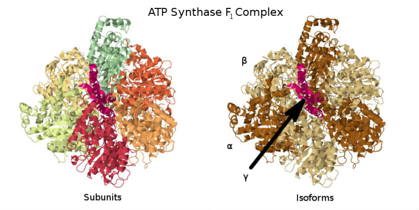
Assumption 3. The modeling of enzyme complex abundance can be tackled by using nested sets of subcomplexes; each enzyme complex consists of multiple subcomplexes, unless it is only a single protein or family of protein isozymes. These subcomplexes are required for the enzyme complex to function (AND relationships), and can be thought of as the division of the complex in to distinct units that each have some necessary function for the complex, with the exception that we do not keep track of the multiplicity of subcomplexes within a complex since this information is, in the current state of affairs, not always known. However, there may be alternative versions of each functional set (given by OR relationships). Eventually, this nested embedding terminates with a single protein or set of peptide isoforms (e.g. isozymes). In the case of ATP Synthase, one of its functional sets is represented by the subcomplex. The subcomplex itself can be viewed as having two immediate subcomplexes: the single (axle) subunit and three identical subcomplexes each made of an and subunit. Each pair works together to bind ADP and catalyze the reaction [36]. The subcomplex itself then has two subcomplexes composed of just an subunit on the one hand and the subunit on the other. It is obvious that one of these base-level functional subcomplexes (in this example, either or ) will be in most limited supply, and that it will best represent the overall enzyme complex abundance (discounting the issues of multiplicity for , see Assumption 4).
The hierarchical structure just described, when written out in Boolean, will give a rule in CNF (conjunctive normal form), or more specifically (owing to the lack of negations), clausal normal form, where a clause is a disjunction of literals (genes). This is because all relations are ANDs (conjunctions), except possibly at the inner-most subcomplexes that have alternative isoforms, which are expressed as ORs (disjunctions). Since GPR rules alone only specify the requirements for enzyme complex formation, we will see that not all forms of Boolean rules are equally useful in evaluating the enzyme complex abundance, but we have established the assumptions in Table 2 and an alternative and logically equivalent rule [16] under which we can estimate enzyme complex copy number.
| Table 2. Assumptions in GPR-based Enzyme Complex Formation |
| 1. Expression values are highly correlated with the copy numbers of their corresponding peptide isoforms. 2. Protein isoforms contributing to isozymes are considered part of the same enzyme complex. 3. Any enzyme complex can be described as a hierarchical subset of (possibly redundant) subcomplexes; redundant subcomplexes, as elaborated in (4), are not currently modeled. 4. Assume one copy of peptide per complex; exact isoform stoichiometry is not considered. 5. With the exception of complexes having identical rules (i.e. the same complex listed for different reactions), each copy of a peptide is available for all complexes in the model. 6. There is only one active site per enzyme complex. 7. We assume that different pathways have similar flux sensitivities with respect to their enzyme abundances. 8. If a particular subcomplex can be catalyzed by A and it can also be catalyzed by A and B (e.g. B acts as a regulatory unit, as in holoenzymes), this just simplifies to A once expression values are substituted in. Similarly, allosteric regulation is not modeled. Relatedly, there are no NOT operations in GPR rules (just ANDs and ORs). 9. Enzyme complexes form without the assistance of protein chaperones and formation is not coupled to other reactions. 10. Post-translational modifications do not affect complex formation. 11. Rate of formation and degradation of complexes doesn’t play a role, since we assume steady-state. |
There is no guarantee that a GPR rule has been written down with this hierarchical structure in mind, though it is likely the case much of the time as it is a natural way to model complexes. However, any GPR rule can be interpreted in the context of this hierarchical view due to the existence of a logically equivalent CNF rule for any non-CNF rule, and it is obvious that logical equivalence is all that is required to check for enzyme complex formation when exact isoform stoichiometry is unknown. As an example, we consider another common formulation for GPR rules, and a way to think about enzyme structure—disjunctive normal form (DNF). A DNF rule is a disjunctive list of conjunctions of peptide isoforms, where each conjunction is some variation of the enzyme complex due to substituting in different isoforms for some of the required subunits. A rule with a more complicated structure and compatible isoforms across subcomplexes may be written more succinctly in CNF, whereas a rule with only very few alternatives derived from isoform variants may be represented clearly with DNF. In rare cases, it is possible that a GPR rule is written in neither DNF or CNF, perhaps because neither of these two alternatives above are strictly the case, and some other rule is more succinct.
Assumptions 4, 5 and 6. One active site per enzyme complex implies a single complex can only catalyze one reaction at a time. Multimeric complexes with one active site per identical subunit would be considered as one enzyme complex per subunit in this model. Note that it is possible for an enzyme complex to catalyze different reactions. In fact, some transporter complexes can transfer many different metabolites across a lipid bilayer—up to 294 distinct reactions in the reversible model for solute carrier family 7 (Gene ID 9057). Another example is the ligation or hydrolysis of nucleotide, fatty acid, or peptide chains, where chains of different length may all be substrates or products of the same enzyme complex. While we do not explicitly consider these in in the minimum disjunction algorithm, these redundancies are taken into account subsequently in Algorithm 3.1.
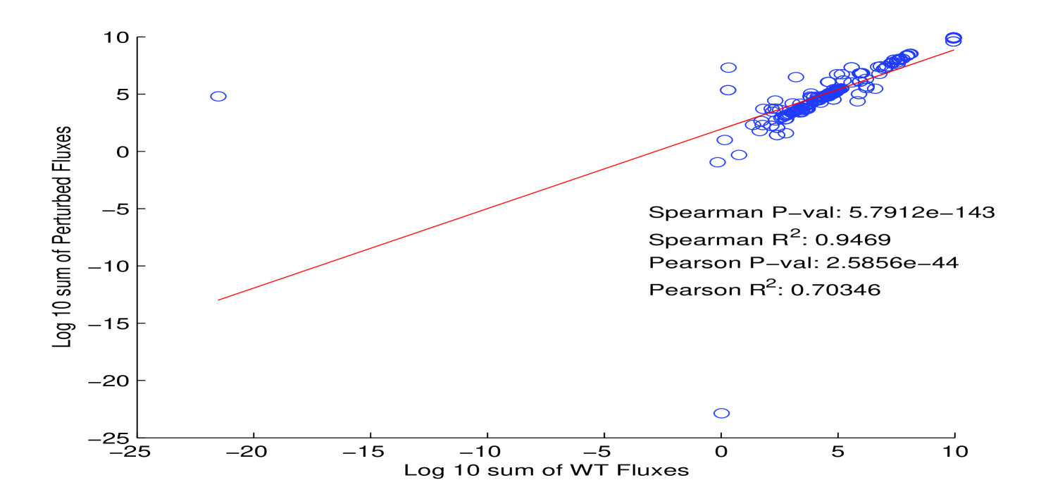
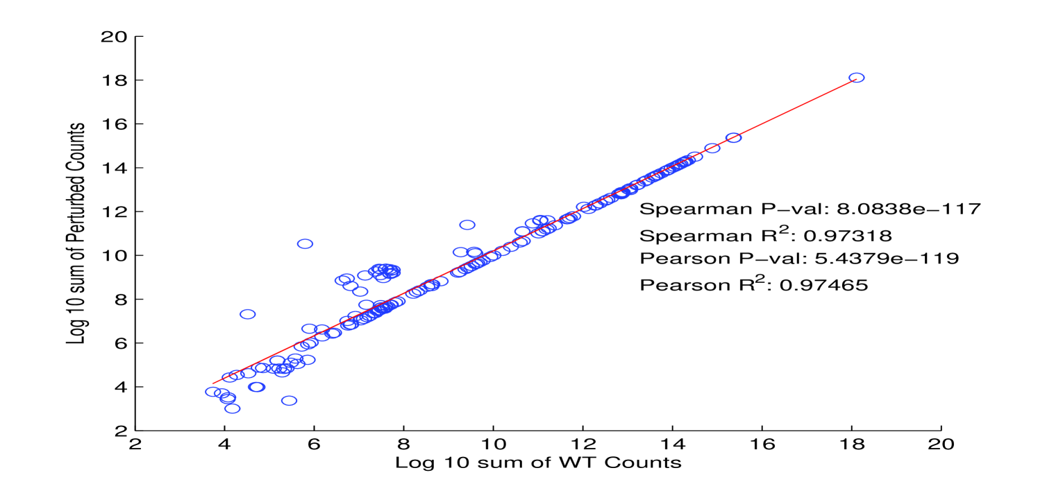
In order to explore the effect that stoichiometry of protein complexes can have on metabolism, we compared time series aggregates of fluxes and metabolite counts from a whole cell model of Mycoplasma genitalium [37] in two different conditions (Figure 12). While there are outliers and deviations from perfect correlation, the results indicate that, at least in a whole cell model of M. genitalium, our assumption for protein complex stoichiometry may be acceptable. Nonetheless, we hope to address this assumption at a future date.
What is currently not considered in our process is that some peptide isoforms may find use in completely different complexes, and in some cases, individual peptides may have multiple active sites; in the first case, we assume an unrealistic case of superposition where the isoform can simultaneously function in more than one complex. The primary reason we have not tackled this problem is because exact subunit stoichiometry of most enzyme complexes is not accurately known, but an increasing abundance of data on BRENDA [38] gives some hope to this problem. A recent E. coli metabolic model incorporating the metabolism of all known gene products [39] also includes putative enzyme complex stoichiometry in GPR rules. For the second point, there are a few enzymes where a single polypeptide may have multiple active sites (e.g. fatty acid synthase), and this is not currently taken into account in our model. One way that we may take this into account has been illustrated online by one of the authors [40].
Assumption 8. We do not make any special assumptions requiring symmetry of an isoform within a complex. For instance, the example in assumption 8 shows how you might have one subcomponent composed of a single isoform, and another subcomponent composed of that gene in addition to another isoform. In this case, it is simply reduced to being the first gene only that is required, since clearly the second is strictly optional. That isn’t to say that the second gene may not have some metabolic effect, such as (potentially) aiding in structural ability or altering the catalytic rate, but it should have no bearing on the formation of a functional catalytic complex. Holoenzymes—enzymes with metabolic cofactors or protein subunits that have a regulatory function for the complex—would likely be the only situation where this type of rule might need to be considered in more detail. But in the absence of detailed kinetic information, this consideration (much like allosteric regulation) is not useful.
No additional algorithmic considerations are needed, as this is a by-product of the conversion to CNF. For instance, take the following example where the second conjunction has the redundant gene :
Distributing during the process of conversion to CNF results in:
Because every disjunction with more than one literal is in conjunction with another disjunction with only one of its literals, the disjunction with fewer literals will be the minimum of the two once evaluated. This applies to both of the singleton disjunctions and , so all other disjunctions will effectively be ignored (it is up to the implementer whether the redundant sub-expressions are removed before evaluation):
Assumption 7. Another important biochemical assumption is that reactions should operate in a regime where they are sensitive to changes in the overall enzyme level in the pathways that they belong in [24, 25]. This is perhaps the most important issue to be explored further for methods like this, since if it is not true, some other adjustment factor would be needed to make the method realistic. For instance, if all reactions in a pathway are operating far below , but it is not the case in another pathway, the current method does not have information on this, and will try to put more flux through the first pathway than should be the case.
Assumptions 9, 10 and 11. Due to the quickness, stability, and energetic favorability of enzyme complex formation, the absence of chaperones or coupled metabolic reactions required for complex formation may be reasonable assumptions, but further research is warranted [37]. Additionally, as in metabolism, we assume a steady state for complex formation, so that rate laws regarding complex formation aren’t needed. However, further research may be warranted to investigate the use of a penalty for complex levels based on mass action and protein-docking information. Requisite to this would be addressing assumption 4. It would be surprising (but not impossible) if such a penalty were very large due to the cost this would imply for many of the large and important enzyme complexes present in all organisms [41]. A more serious consideration may be that information on post-translational modification is not currently considered. Post-translational modification is highly context-specific and the relevant data is not as cheap to get as expression data, so it may be some time before it can be integrated into the modeling framework.
9 Benchmarking of solvers
We have exclusively used the Gurobi solver [42] for this work, which is a highly competitive solver that employs by default a parallel strategy to solving problems: a different algorithm is run simultaneously, and as soon as one algorithm finished the others terminate. Of course, if there is a clear choice of algorithm for a particular problem class, this should be used in production settings to avoid wasted CPU time and memory. In order to address this, we benchmarked the three non-parallel solver methods in Gurobi (since parallel solvers simply use multiple methods simultaneously). The exception to this rule is the Barrier method, which can use multiple threads, but in practice for our models appears to use no more than about 6 full CPU cores simultaneously for our models. Our results for Yeast 5 and Yeast 7 with minimal directionality constraints [22, 8, 18] and Human Recon 2 [19] are shown in Table 3).
| Model | Primal-Simplex | Dual-Simplex | Barrier |
|---|---|---|---|
| Yeast 5.21 (2,061 reactions) | |||
| Yeast 7.0 (3,498 reactions) | |||
| Human 2.03 (7,440 reactions) |
We found that in Yeast 7 with the primal-simplex solver, there is a chance the solver will fail to find a feasible solution. We verified that this is a numeric issue in Gurobi and can be fixed by setting the Gurobi parameter MarkowitzTol to a larger value (which decreases time-efficiency but limits the numerical error in the simplex algorithm). In practice, failure for the algorithm to converge at an advanced iteration is rare and is not always a major problem (since the previous flux estimate by the advanced iteration should already be quite good), but it is certainly undesirable; a warning message will be printed by falcon if this occurs, at which point parameter settings can be investigated. In the future, we plan to improve falcon so that parameters will be adjusted as needed during progression of the algorithm after finding a good test suite of models and data. For now, we use the dual-simplex solver, for which we have always had good results.
Because the number of iterations depends non-trivially on the model and the expression data, it may be more helpful to look at the average time per iteration in the above examples (Table 4).
| Model | Primal-Simplex | Dual-Simplex | Barrier |
|---|---|---|---|
| Yeast 5.21 (2,061 reactions) | |||
| Yeast 7.0 (3,498 reactions) | |||
| Human 2.03 (7,440 reactions) |
Given the above rare trouble with primal simplex solver the universal best performance enjoyed by the dual-simplex method (Tables 3 and 4), we would advise the dual-simplex algorithms, all else being equal. The dual-simplex method is also recommended for memory-efficiency by Gurobi documentation, but we did not observe any differences in memory for different solver methods.
All timing analyses were performed on a system with four 8-core AMD Opteron™ 6136 processors operating at 2.4 GHz. Figure 6, Table 1, and Tables 3 and 4 used a single unperturbed expression file per species (S. cerevisiae and H. sapiens; see timingAnalysis.m for details). Values were averaged across 32 replicates. Note that the iMAT method is formulated as a mixed integer program [14], and was able to use additional parallelization of the solver [42] whereas other methods only used a single core (our system had 32 cores and iMAT with Gurobi would use all of them). Tables 3 and 4 used multivariate log-normal noise multiplied by the original expression vector to introduce more variance in the calculations; the human models were tested with 100 replicates and the yeast models with 500 replicates.
10 Generation of figures and tables
All non-trivial figures can be generated using MATLAB scripts found in the analysis/figures subdirectory of the FALCON installation. In particular, figures should be generated through the master script makeMethodFigures.m by calling makeMethodFigures(figName) where figName has a name corresponding to the desired figure. In some cases, some MATLAB .mat files will need to be generated by other scripts first; see the plotting scripts or the subsections below for details. An example is to make the scatter plots showing the difference between running falcon with enzyme abundances determined by direct evaluation or the minimum disjunction algorithm; all three scatter plots are generated with the command makeMethodFigures('fluxCmpScatter'). Note that, as written, this requires a graphical MATLAB session.
Several figures can be generated that are related to comparing human proteomic and transcriptomic data by executing the script proteomic_file_make.py in the analysis/nci60 subdirectory; this includes Figure 10.
Comparison of the effects of the employed enzyme complexation methods were evaluated using compareEnzymeExpression.m and compareFluxByRGroup.m. Comparison of reaction groups was performed in compareFluxByRGroup.m.
10.1 Timing analyses
All timing analyses were performed on a system with four 8-core AMD Opteron™ 6136 processors operating at 2.4 GHz. Figure 6 and Table 1 used unperturbed expression data; see yeastResults.m for details). Values for the FALCON method were averaged across 32 replicates, while values for the Lee et al. 8 method were averaged across 8 replicates. Human timing analyses were performed using methodTimer.m with 8 replicates.
10.2 Data sources
Enzyme complexation comparisons were performed on proteomics data from Gholami et al. 21 (Human; 786-O cell line) and Picotti et al. 20 (yeast; BY strain), and on RNA-Seq data from Lee et al. 8 (yeast; 75% max condition). Human proteomic and trascriptomic data used for comparison in Figure 10 were taken from Gholami et al. 21.
References
- Shestov et al. [2013] Alexander A Shestov, Brandon Barker, Zhenglong Gu, and Jason W Locasale. Computational approaches for understanding energy metabolism. Wiley Interdisciplinary Reviews: Systems Biology and Medicine, 5(6):733–750, July 2013. ISSN 1939-005X. doi: 10.1002/wsbm.1238. URL http://dx.doi.org/10.1002/wsbm.1238.
- Lewis et al. [2012] Nathan E Lewis, Harish Nagarajan, and Bernhard Ø Palsson. Constraining the metabolic genotype-phenotype relationship using a phylogeny of in silico methods. Nature reviews. Microbiology, 10(4):291–305, April 2012. ISSN 1740-1534. doi: 10.1038/nrmicro2737. URL http://www.ncbi.nlm.nih.gov/pubmed/22367118.
- Schuetz et al. [2012] R. Schuetz, N. Zamboni, M. Zampieri, M. Heinemann, and U. Sauer. Multidimensional Optimality of Microbial Metabolism. Science, 336(6081):601–604, May 2012. ISSN 0036-8075. doi: 10.1126/science.1216882. URL http://www.sciencemag.org/cgi/doi/10.1126/science.1216882.
- Fong and Palsson [2004] Stephen S Fong and Bernhard Ø Palsson. Metabolic gene-deletion strains of Escherichia coli evolve to computationally predicted growth phenotypes. Nature genetics, 36(10):1056–8, October 2004. ISSN 1061-4036. doi: 10.1038/ng1432. URL http://www.ncbi.nlm.nih.gov/pubmed/15448692.
- Pirkmajer and Chibalin [2011] Sergej Pirkmajer and Alexander V Chibalin. Serum starvation: caveat emptor. American journal of physiology. Cell Physiology., 301(2):C272–C279, July 2011. URL http://ajpcell.physiology.org/highwire/citation/1105/mendeley.
- Blazier and Papin [2012] Anna S Blazier and Jason a Papin. Integration of expression data in genome-scale metabolic network reconstructions. Frontiers in physiology, 3(August):299, January 2012. ISSN 1664-042X. doi: 10.3389/fphys.2012.00299. URL http://www.pubmedcentral.nih.gov/articlerender.fcgi?artid=3429070\&tool=pmcentrez\&rendertype=abstract.
- Segrè et al. [2002] Daniel Segrè, Dennis Vitkup, and George M Church. Analysis of optimality in natural and perturbed metabolic networks. Proceedings of the National Academy of Sciences of the United States of America, 99(23):15112–7, November 2002. ISSN 0027-8424. doi: 10.1073/pnas.232349399. URL http://www.pubmedcentral.nih.gov/articlerender.fcgi?artid=137552\&tool=pmcentrez\&rendertype=abstract.
- Lee et al. [2012] Dave Lee, Kieran Smallbone, Warwick B Dunn, Ettore Murabito, Catherine L Winder, Douglas B Kell, Pedro Mendes, and Neil Swainston. Improving metabolic flux predictions using absolute gene expression data. BMC systems biology, 6(1):73, January 2012. ISSN 1752-0509. doi: 10.1186/1752-0509-6-73. URL http://www.pubmedcentral.nih.gov/articlerender.fcgi?artid=3477026\&tool=pmcentrez\&rendertype=abstract.
- Colijn et al. [2009] Caroline Colijn, Aaron Brandes, Jeremy Zucker, Desmond S Lun, Brian Weiner, Maha R Farhat, Tan-Yun Cheng, D Branch Moody, Megan Murray, and James E Galagan. Interpreting Expression Data with Metabolic Flux Models: Predicting Mycobacterium tuberculosis Mycolic Acid Production. PLoS Comput Biol, 5(8):e1000489, 2009. doi: 10.1371/journal.pcbi.1000489. URL http://dx.doi.org/10.1371/journal.pcbi.1000489.
- [10] Eli Bogart and Christopher R Myers. Multiscale metabolic modeling of C4 plants: connecting nonlinear genome-scale models to leaf-scale metabolism in developing maize leaves. URL http://arxiv.org/art/1502.07969.
- Shlomi et al. [2005] Tomer Shlomi, Omer Berkman, and Eytan Ruppin. Regulatory on/off minimization of metabolic flux. Proceedings of the National Academy of Sciences, 102(21):7695–7700, 2005.
- Boyd and Vandenberghe [2004] Stephen Boyd and Lieven Vandenberghe. Convex Optimization. Cambridge University Press, New York, 2004. ISBN 978-0-521-83378-3. URL http://www.stanford.edu/~boyd/cvxbook/.
- Becker and Palsson [2008] Scott A Becker and Bernhard Ø Palsson. Context-specific metabolic networks are consistent with experiments. PLoS computational biology, 4(5):1–10, May 2008. ISSN 1553-7358. doi: 10.1371/journal.pcbi.1000082. URL http://www.pubmedcentral.nih.gov/articlerender.fcgi?artid=2366062\&tool=pmcentrez\&rendertype=abstract.
- Shlomi et al. [2008] Tomer Shlomi, Moran N Cabili, Markus J Herrgård, Bernhard Ø Palsson, and Eytan Ruppin. Network-based prediction of human tissue-specific metabolism. Nature biotechnology, 26(9):1003–10, September 2008. ISSN 1546-1696. doi: 10.1038/nbt.1487. URL http://www.ncbi.nlm.nih.gov/pubmed/18711341.
- Jüschke et al. [2013] Christoph Jüschke, Ilse Dohnal, Peter Pichler, Heike Harzer, Remco Swart, Gustav Ammerer, Karl Mechtler, and Juergen A Knoblich. Transcriptome and proteome quantification of a tumor model provides novel insights into post-transcriptional gene regulation. Genome Biology, 14(11):1–33, 2013. ISSN 1465-6906. doi: 10.1186/gb-2013-14-11-r133. URL http://genomebiology.com/2013/14/11/R133.
- Russell and Norvig [2009] Stuart Russell and Peter Norvig. Artificial Intelligence: A Modern Approach, 3rd edition. Prentice Hall, 2009. ISSN 0269-8889. doi: 10.1017/S0269888900007724. URL http://portal.acm.org/citation.cfm?id=1671238\&coll=DL\&dl=GUIDE\&CFID=190864501\&CFTOKEN=29051579$\backslash$npapers2://publication/uuid/4B787E16-89F6-4FF7-A5E5-E59F3CFEFE88.
- Orth et al. [2011] Jeffrey D Orth, Tom M Conrad, Jessica Na, Joshua a Lerman, Hojung Nam, Adam M Feist, and Bernhard Ø Palsson. A comprehensive genome-scale reconstruction of Escherichia coli metabolism—2011. Molecular Systems Biology, 7(535):1–9, October 2011. ISSN 1744-4292. doi: 10.1038/msb.2011.65. URL http://www.nature.com/doifinder/10.1038/msb.2011.65.
- Aung et al. [2013] Hnin W Aung, Susan A Henry, and Larry P Walker. Revising the Representation of Fatty Acid, Glycerolipid, and Glycerophospholipid Metabolism in the Consensus Model of Yeast Metabolism. Industrial Biotechnology, 9(4):215–228, August 2013. ISSN 1550-9087. doi: 10.1089/ind.2013.0013. URL http://online.liebertpub.com/doi/abs/10.1089/ind.2013.0013.
- Thiele et al. [2013] Ines Thiele, Neil Swainston, Ronan M T Fleming, Andreas Hoppe, Swagatika Sahoo, Maike K Aurich, Hulda Haraldsdottir, Monica L Mo, Ottar Rolfsson, Miranda D Stobbe, Stefan G Thorleifsson, Rasmus Agren, Christian Bölling, Sergio Bordel, Arvind K Chavali, Paul Dobson, Warwick B Dunn, Lukas Endler, David Hala, Michael Hucka, Duncan Hull, Daniel Jameson, Neema Jamshidi, Jon J Jonsson, Nick Juty, Sarah Keating, Intawat Nookaew, Nicolas Le Novère, Naglis Malys, Alexander Mazein, Jason A Papin, Nathan D Price, Anatoly Sorokin, Johannes H G M Van Beek, Dieter Weichart, Igor Goryanin, and Jens Nielsen. A community-driven global reconstruction of human metabolism. Nature biotechnology, 31(March 2013):1–9, 2013. doi: 10.1038/nbt.2488.
- Picotti et al. [2013] Paola Picotti, Mathieu Clement-Ziza, Henry Lam, David S Campbell, Alexander Schmidt, Eric W Deutsch, Hannes Rost, Zhi Sun, Oliver Rinner, Lukas Reiter, Qin Shen, Jacob J Michaelson, Andreas Frei, Simon Alberti, Ulrike Kusebauch, Bernd Wollscheid, Robert L Moritz, Andreas Beyer, and Ruedi Aebersold. A complete mass-spectrometric map of the yeast proteome applied to quantitative trait analysis. Nature, 494(7436):266–270, February 2013. ISSN 0028-0836. URL http://dx.doi.org/10.1038/nature11835http://www.nature.com/nature/journal/v494/n7436/abs/nature11835.html\#supplementary-information.
- Gholami et al. [2013] Amin Moghaddas Gholami, Hannes Hahne, Zhixiang Wu, Florian Johann Auer, Chen Meng, Mathias Wilhelm, and Bernhard Kuster. Global Proteome Analysis of the NCI-60 Cell Line Panel. Cell Reports, 4(3):609–620, August 2013. URL http://linkinghub.elsevier.com/retrieve/pii/S221112471300380X.
- Heavner et al. [2012] Benjamin D Heavner, Kieran Smallbone, Brandon Barker, Pedro Mendes, and Larry P Walker. Yeast 5 - an expanded reconstruction of the Saccharomyces cerevisiae metabolic network. BMC systems biology, 6(1):55, January 2012. ISSN 1752-0509. doi: 10.1186/1752-0509-6-55. URL http://www.pubmedcentral.nih.gov/articlerender.fcgi?artid=3413506\&tool=pmcentrez\&rendertype=abstract.
- Shlomi et al. [2011] Tomer Shlomi, Tomer Benyamini, Eyal Gottlieb, Roded Sharan, and Eytan Ruppin. Genome-scale metabolic modeling elucidates the role of proliferative adaptation in causing the Warburg effect. PLoS computational biology, 7(3):e1002018, March 2011. ISSN 1553-7358. doi: 10.1371/journal.pcbi.1002018. URL http://www.pubmedcentral.nih.gov/articlerender.fcgi?artid=3053319\&tool=pmcentrez\&rendertype=abstract.
- Bennett et al. [2009] Bryson D Bennett, Elizabeth H Kimball, Melissa Gao, Robin Osterhout, Stephen J Van Dien, and Joshua D Rabinowitz. Absolute metabolite concentrations and implied enzyme active site occupancy in Escherichia coli. Nature chemical biology, 5(8):593–599, August 2009. ISSN 1552-4450. URL http://dx.doi.org/10.1038/nchembio.186http://www.nature.com/nchembio/journal/v5/n8/suppinfo/nchembio.186\_S1.html.
- Chubukov et al. [2013] Victor Chubukov, Markus Uhr, Ludovic Le Chat, Roelco J Kleijn, Matthieu Jules, Hannes Link, Stephane Aymerich, Jorg Stelling, and Uwe Sauer. Transcriptional regulation is insufficient to explain substrate-induced flux changes in Bacillus subtilis. Molecular systems biology, 9, November 2013. URL http://dx.doi.org/10.1038/msb.2013.6610.1038/msb.2013.66.
- Chandrasekaran and Price [2010] Sriram Chandrasekaran and Nathan D Price. Probabilistic integrative modeling of genome-scale metabolic and regulatory networks in Escherichia coli and Mycobacterium tuberculosis. Proceedings of the National Academy of Sciences of the United States of America, 107(41):17845–50, October 2010. ISSN 1091-6490. doi: 10.1073/pnas.1005139107. URL http://www.pubmedcentral.nih.gov/articlerender.fcgi?artid=2955152\&tool=pmcentrez\&rendertype=abstract.
- Reed et al. [2006] Jennifer L Reed, Trina R Patel, Keri H Chen, Andrew R Joyce, Margaret K Applebee, Christopher D Herring, Olivia T Bui, Eric M Knight, Stephen S Fong, and Bernhard Ø Palsson. Systems approach to refining genome annotation. Proceedings of the National Academy of Sciences, 103(46):17480–17484, 2006. doi: 10.1073/pnas.0603364103. URL http://www.pnas.org/content/103/46/17480.abstract.
- Mitra et al. [2013] Koyel Mitra, Anne-Ruxandra Carvunis, Sanath Kumar Ramesh, and Trey Ideker. Integrative approaches for finding modular structure in biological networks. Nature reviews. Genetics, 14(10):719–732, October 2013. ISSN 1471-0056. URL http://dx.doi.org/10.1038/nrg355210.1038/nrg3552%****␣falcon_main.bbl␣Line␣300␣****http://www.nature.com/nrg/journal/v14/n10/abs/nrg3552.html\#supplementary-information.
- Plata et al. [2012] Germán Plata, Tobias Fuhrer, Tzu-Lin Hsiao, Uwe Sauer, and Dennis Vitkup. Global probabilistic annotation of metabolic networks enables enzyme discovery. Nature chemical biology, 8(10):848–854, October 2012. ISSN 1552-4450. URL http://dx.doi.org/10.1038/nchembio.1063http://www.nature.com/nchembio/journal/v8/n10/abs/nchembio.1063.html\#supplementary-information.
- Gowen and Fong [2010] Christopher M Gowen and Stephen S Fong. Genome-scale metabolic model integrated with RNAseq data to identify metabolic states of Clostridium thermocellum. Biotechnology Journal, 5(7):759–767, July 2010. ISSN 1860-7314. doi: 10.1002/biot.201000084. URL http://dx.doi.org/10.1002/biot.201000084.
- Jain et al. [2012] Mohit Jain, Roland Nilsson, Sonia Sharma, Nikhil Madhusudhan, Toshimori Kitami, Amanda L Souza, Ran Kafri, Marc W Kirschner, Clary B Clish, and Vamsi K Mootha. Metabolite Profiling Identifies a Key Role for Glycine in Rapid Cancer Cell Proliferation. Science, 336(6084):1040–1044, May 2012. doi: 10.1126/science.1218595. URL http://www.sciencemag.org/content/336/6084/1040.abstract.
- Nagaraj et al. [2011] Nagarjuna Nagaraj, Jacek R Wisniewski, Tamar Geiger, Juergen Cox, Martin Kircher, Janet Kelso, Svante Paabo, and Matthias Mann. Deep proteome and transcriptome mapping of a human cancer cell line. Molecular systems biology, 7, November 2011. URL http://dx.doi.org/10.1038/msb.2011.81http://www.nature.com/msb/journal/v7/n1/suppinfo/msb201181\_S1.html.
- Gibbons et al. [2000] Clyde Gibbons, Martin G Montgomery, Andrew G W Leslie, and John E Walker. The structure of the central stalk in bovine F1-ATPase at 2.4 A resolution. Nat Struct Mol Biol, 7(11):1055–1061, November 2000. ISSN 1072-8368. URL http://dx.doi.org/10.1038/80981.
- Bernstein et al. [1978] Frances C Bernstein, Thomas F Koetzle, Graheme J B Williams, Edgar F Meyer Jr., Michael D Brice, John R Rodgers, Olga Kennard, Takehiko Shimanouchi, and Mitsuo Tasumi. The protein data bank: A computer-based archival file for macromolecular structures. Archives of Biochemistry and Biophysics, 185(2):584–591, January 1978. ISSN 0003-9861. doi: http://dx.doi.org/10.1016/0003-9861(78)90204-7. URL http://www.sciencedirect.com/science/article/pii/0003986178902047.
- Gezelter et al. [2013] Dan Gezelter, Bradley A Smith, and Egon Willighagen. Jmol: an open-source Java viewer for chemical structures in 3D, 2013. URL http://www.jmol.org/.
- Oster and Wang [2003] George Oster and Hongyun Wang. Rotary protein motors. Trends in cell biology, 13(3):114–121, March 2003. URL http://linkinghub.elsevier.com/retrieve/pii/S0962892403000047.
- Karr et al. [2012] Jonathan R Karr, Jayodita C Sanghvi, Derek N Macklin, Miriam V Gutschow, Jared M Jacobs, Benjamin Bolival, Nacyra Assad-Garcia, John I Glass, and Markus W Covert. A whole-cell computational model predicts phenotype from genotype. Cell, 150(2):389–401, July 2012. ISSN 1097-4172. doi: 10.1016/j.cell.2012.05.044. URL http://www.ncbi.nlm.nih.gov/pubmed/22817898.
- Schomburg et al. [2013] Ida Schomburg, Antje Chang, Sandra Placzek, Carola Söhngen, Michael Rother, Maren Lang, Cornelia Munaretto, Susanne Ulas, Michael Stelzer, Andreas Grote, Maurice Scheer, and Dietmar Schomburg. BRENDA in 2013: integrated reactions, kinetic data, enzyme function data, improved disease classification: new options and contents in BRENDA. Nucleic Acids Research, 41(D1):D764–D772, January 2013. doi: 10.1093/nar/gks1049. URL http://nar.oxfordjournals.org/content/41/D1/D764.abstract.
- O’Brien et al. [2013] Edward J O’Brien, Joshua A Lerman, Roger L Chang, Daniel R Hyduke, and Bernhard Ø Palsson. Genome-scale models of metabolism and gene expression extend and refine growth phenotype prediction. Molecular systems biology, 9, October 2013. URL http://dx.doi.org/10.1038/msb.2013.5210.1038/msb.2013.52.
- Smallbone [2014] Kieran Smallbone. From genes to fluxes, 2014. URL https://u003f.wordpress.com/2014/02/19/from-genes-to-fluxes-2/.
- Nelson and Cox [2008] David L Nelson and Michael M Cox. Lehninger Principles of Biochemistry. W.H. Freeman, New York, NY, USA, 5 edition, 2008. ISBN 071677108X. URL http://www.amazon.com/Lehninger-Principles-Biochemistry-Fourth-Nelson/dp/0716743396.
- Inc. [2013] Gurobi Optimization Inc. Gurobi Optimizer Reference Manual, 2013. URL http://www.gurobi.com.