2128 \lmcsheadingLABEL:LastPageSep. 27, 2021Apr. 24, 2025
[a] [b] [a]
A robust graph-based approach to observational equivalence
Abstract.
We propose a new step-wise approach to proving observational equivalence, and in particular reasoning about fragility of observational equivalence. Our approach is based on what we call local reasoning. The local reasoning exploits the graphical concept of neighbourhood, and it extracts a new, formal, concept of robustness as a key sufficient condition of observational equivalence. Moreover, our proof methodology is capable of proving a generalised notion of observational equivalence. The generalised notion can be quantified over syntactically restricted contexts instead of all contexts, and also quantitatively constrained in terms of the number of reduction steps. The operational machinery we use is given by a hypergraph-rewriting abstract machine inspired by Girard’s Geometry of Interaction. The behaviour of language features, including function abstraction and application, is provided by hypergraph-rewriting rules. We demonstrate our proof methodology using the call-by-value lambda-calculus equipped with (higher-order) state.
1. Introduction
1.1. Context and motivation
Observational equivalence [MJ69] is an old and central question in the study of programming languages. Two executable programs are observationally equivalent when they have the same behaviour. Observational equivalence between two program fragments (aka. terms) is the smallest congruence with respect to arbitrary program contexts. By formally establishing observational equivalence, one can justify compiler optimisation, and verify and validate programs.
There are two mathematical challenges in proving observational equivalence. Firstly, universal quantification over contexts is unwieldy. This has led to various indirect approaches to observational semantics. As an extremal case, denotational semantics provides a model-theoretic route to observational equivalence. There are also hybrid approaches that employ both denotational and operational techniques, such as Kripke logical relations [Sta85] and trace semantics [JR05]. Moreover, an operational and coinductive approach exists, under the name of applicative bisimilarity [Abr90].
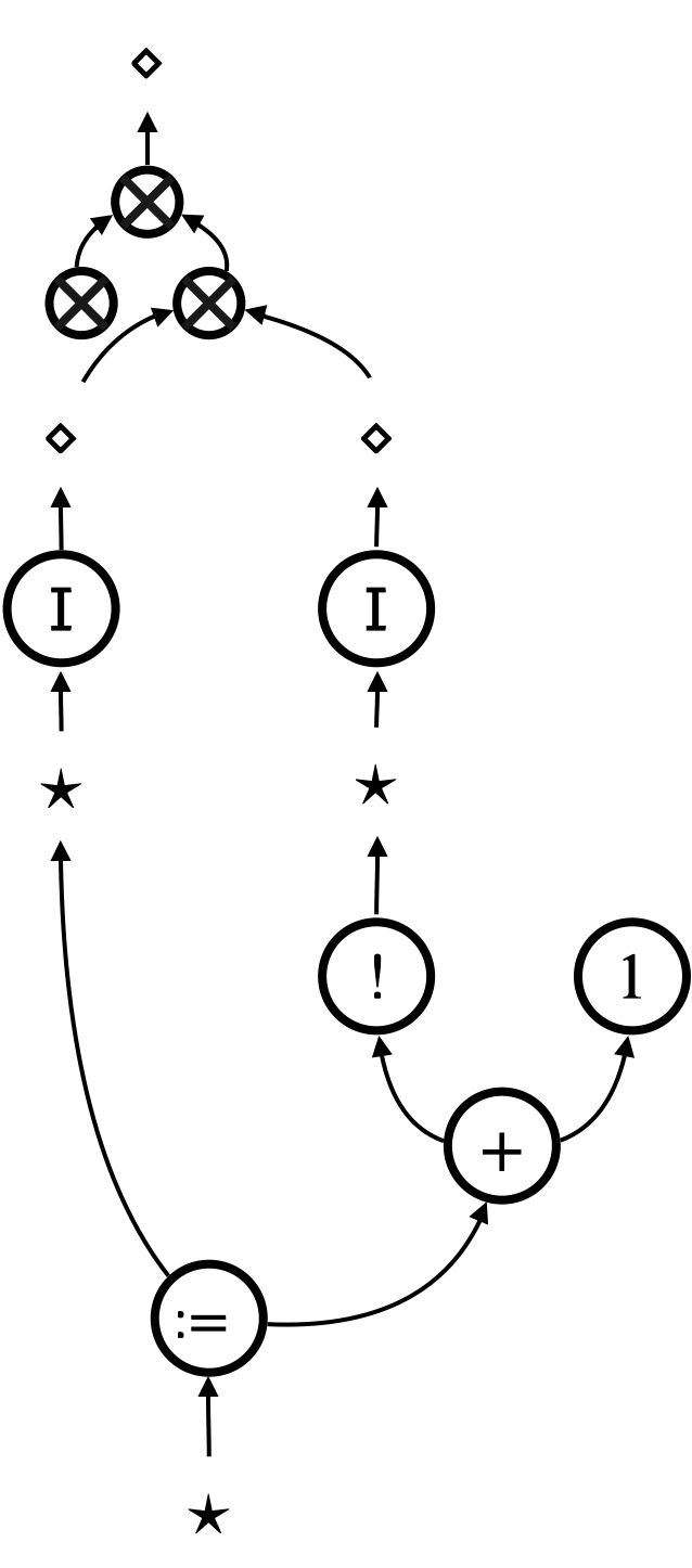
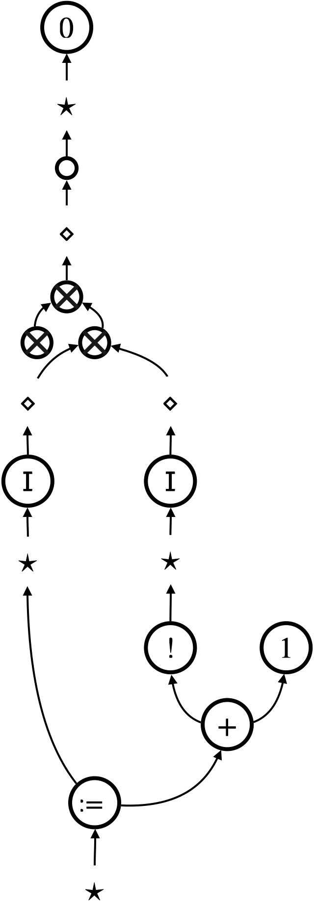
The second challenge is fragility of observational equivalence. The richer a programming language is, the more discriminating power program contexts have and hence the less observational equivalences hold in the language. For example, the beta-law is regarded as the fundamental observational equivalence in functional programming. However, it can be violated in the presence of a memory inspection feature like the one provided by the OCaml garbage-collection (Gc) module. A function that returns the size of a given program enables contexts to distinguish from , for example111See a concrete example written in OCaml, on the online platform Try It Online: https://bit.ly/3TqnGOW.
The fragility of observational equivalence extends to its proof methodologies. There have been studies of the impact that language features have on semantics and hence on proof methodologies for observational equivalence. The development of game semantics made it possible to give combinatorial, syntax-independent and orthogonal characterisations for classes of features such as state and control, e.g. the so-called “Abramsky cube” [Abr97, Ghi23], or to replace the syntactic notion of context by an abstracted adversary [GT12]. A classification [DNB12] and characterisation [DNRB10] of language features and their impact on reasoning has also been undertaken using logical relations. Applicative bisimilarity has been enriched to handle effects such as algebraic effects, local state, names and continuations [SKS07, KLS11, DGL17, SV18].
1.2. Overview and contribution
What is missing and desirable seems a general semantical framework with which one can directly analyse fragility, or robustness, of observational equivalences. To this end, we introduce a graphical abstract machine that implements focussed hypernet rewriting. We then propose a radically new approach to proving observational equivalence that is based on step-wise and local reasoning and centred around a concept of robustness. All these concepts will be rigorously defined in the paper.
The main contribution of the paper is rather conceptual, showing how the graphical concept of neighbourhood can be exploited to reason about observational equivalence, in a new and advantageous way. The technical development of the paper might seem quite elaborate, but this is because we construct a whole new methodology from scratch: namely, focussed hypernet rewriting and reasoning principles for it. These reasoning principles enable us to analyse fragility, or robustness, of observational equivalences in a formal way.
We introduce and use hypernets to represent (functional) programs with effects. Hypernets are an anonymised version of abstract syntax trees, where variables are simply represented as connections. Formally, hypernets are given by hierarchical hypergraphs. Hierarchy allows a hypergraph to be an edge label recursively. An extensive introduction to hypernets and rewriting of them can be found in the literature [GZ23].
Given a hypernet that represents a term, its evaluation is modelled by step-by-step traversal and update of the hypernet. Traversal steps implement depth-first search on the hypernet for a redex, and each update step triggers application of a rewrite rule to the hypernet. Traversal and update are interwoven strategically using a focus that is simply a dedicated edge passed around the hypernet. Importantly, updates are always triggered by a certain focus, and designed to only happen around the focus. We call this model of evaluation focussed hypernet rewriting.
There are mainly two differences compared with conventional reduction semantics. The first difference is the use of hypernets instead of terms. This makes renaming of variables irrelevant. The second difference is the use of the focus instead of evaluation contexts. In conventional reduction semantics, redexes are identified using evaluation contexts. Whenever the focus triggers an update of a hypernet, its position in the hypernet coincides with where the hole is in an evaluation context.
A new step-wise approach.
This work takes a new coinductive, step-wise, approach to proving observational equivalence. We introduce a novel variant of the weak simulation dubbed counting simulation. We demonstrate that, to prove observational equivalence, it suffices to construct a counting simulation that is closed under contexts by definition. This approach is opposite to the known coinductive approach which uses applicative bisimilarity; one first constructs an applicative bisimulation and then proves that it is a congruence, typically using Howe’s method [How96].
Local reasoning.
In combination with our new step-wise approach, focussed hypernet rewriting facilitates what we call local reasoning. Our key observation is that, to obtain the counting simulation that is closed under contexts by definition, it suffices to simply trace sub-graphs and analyse their interaction with the focus. The interaction can namely be analysed by inspecting updates that happen around the focus and how these updates can interfere with the sub-graphs of interest. The reasoning principal here is the graphical concept of neighbourhood, or graph locality.
The local reasoning is a graph counterpart of analysing interaction between (sub-)terms and contexts using the conventional reduction semantics. In fact, it is not just a counterpart but an enhancement in two directions. Firstly, sub-graphs are more expressive than sub-terms; sub-graphs can represent parts of a program that are not necessarily well-formed. Secondly, the focus can indicate which part of a context is relevant in the interaction between the context and a term, which is not easy to make explicit in the conventional semantics that uses evaluation contexts.
Robustness.
Finally, local reasoning extracts a formal concept of robustness in proving observational equivalence. Robustness is identified as the key sufficient condition that ensures two sub-graphs that we wish to equate interact with updates of a hypernet, which is triggered by the focus, in the same way; for example, if one sub-graph is duplicated (or discarded), the other is also duplicated (or discarded).
The concept of robustness helps us gain insights into fragility of observational equivalence. If robustness of two sub-graphs fails, we obtain a counterexample, which is given by a rewrite rule that interferes with the two sub-graphs in different ways. Let be the two different results of interference (i.e. is the result of updating , and is the result of updating ). There are two possibilities.
-
(1)
The sub-graphs are actually observationally equivalent. In this case, the counterexample suggests that the two different results should first be equated. The observational equivalence we wish to establish is likely to depend on the ancillary observational equivalence .
-
(2)
The observational equivalence fails too. In this case, the counterexample provides the particular computation that violates the equivalence, in terms of a rewrite rule. We can conclude that the language feature that induces the computation violates the observational equivalence.
Generalised contextual equivalence.
Using focussed hypernet rewriting, we propose a generalised notion of contextual equivalence. The notion has two parameters: a class of contexts and a preorder on natural numbers. The first parameter enables us to quantify over syntactically restricted contexts, instead of all contexts as in the standard notion. This can be used to identify a shape of contexts that respects or violates certain observational equivalences, given that not necessarily all arbitrarily generated contexts arise in program execution. The second parameter, a preorder on natural numbers, deals with numbers of steps it takes for program execution to terminate. Taking the universal relation recovers the standard notion of contextual equivalence. Another instance is contextual equivalence with respect to the greater-than-or-equal relation on natural numbers, which resembles the notion of improvement [San95, ADV20, ADV21] that is used to establish equivalence and also to compare efficiency of abstract machines. This instance of contextual equivalence is useful to establish that two programs have the same observable execution result, and also that one program terminates with fewer steps than the other.
1.3. Organisation of the paper
Section 2 provides a gentle introduction to our graph-based approach to modelling program evaluation, and reasoning about observational equivalence with the key concepts of locality and robustness. Section 3 formalises the graphs we use, namely hypernets. The rest of the paper is in two halves.
In the first half, we develop our reasoning framework, targeting the linear lambda-calculus. Although linear lambda-terms have restricted expressive power, they are simple enough to demonstrate the development throughout. Section 4 presents the hypernet representation of linear lambda-terms. Section 5 then presents our operational semantics, i.e. focussed hypernet rewriting. Section 6 formalises it as an abstract machine called universal abstract machine (UAM).
Section 7 sets the target of our proof methodology, introducing the generalised notion of contextual equivalence. Section 8 presents our main technical contributions: it formalises the concept of robustness, and presents our main technical result which is the sufficiency-of-robustness theorem (6).
In the second half, we extend our approach to the general (non-linear) lambda-calculus equipped with store. Section 9 describes how the hypernet representation can be adapted. Section 10 shows how the UAM can be extended accordingly, and presents the copying UAM. Section 11 formalises observational equivalence between lambda-terms by means of contextual equivalence between hypernets. Section 12 then demonstrates our approach by proving some example equivalences for the call-by-value lambda-calculus extended with state. The choice of the language here is pedagogical; our methodology can accommodate other effects as long as they are deterministic.
Finally, Section 13 discusses related and future work, concluding the paper. Some details of proofs are presented in Appendix.
2. A gentle introduction
2.1. Hypernets
Compilers and interpreters deal with programs mainly in the form of an abstract syntax tree (AST) rather than text. It is broadly accepted that such a data structure is easier to manipulate algorithmically. Somewhat curiously perhaps, reduction semantics (or small-step operational semantics), which is essentially a list of rules for program manipulation, is expressed using text rather than the tree form. In contrast, our graph-based semantics is expressed as algorithmic manipulations of the data structure that represents syntax.
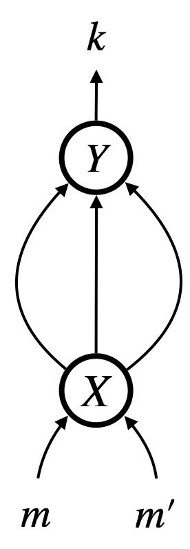
Let us demonstrate our graphical representation, using the beta-law
| (1) |
in the linear lambda-calculus. We use colours to clarify some variable scopes. This law substitutes for the variable , and in doing so, the bound variable has to be renamed to so it does not capture the variable in .
Our first observation is that ASTs are not satisfactory to represent syntax, when it comes to define operational semantics. They contain more syntactic details than necessary, namely by representing variables using names. This makes an operation on terms like substitution a global affair. To avoid variable capturing, substitution needs to clarify the scope of each variable and appropriately rename some variables.
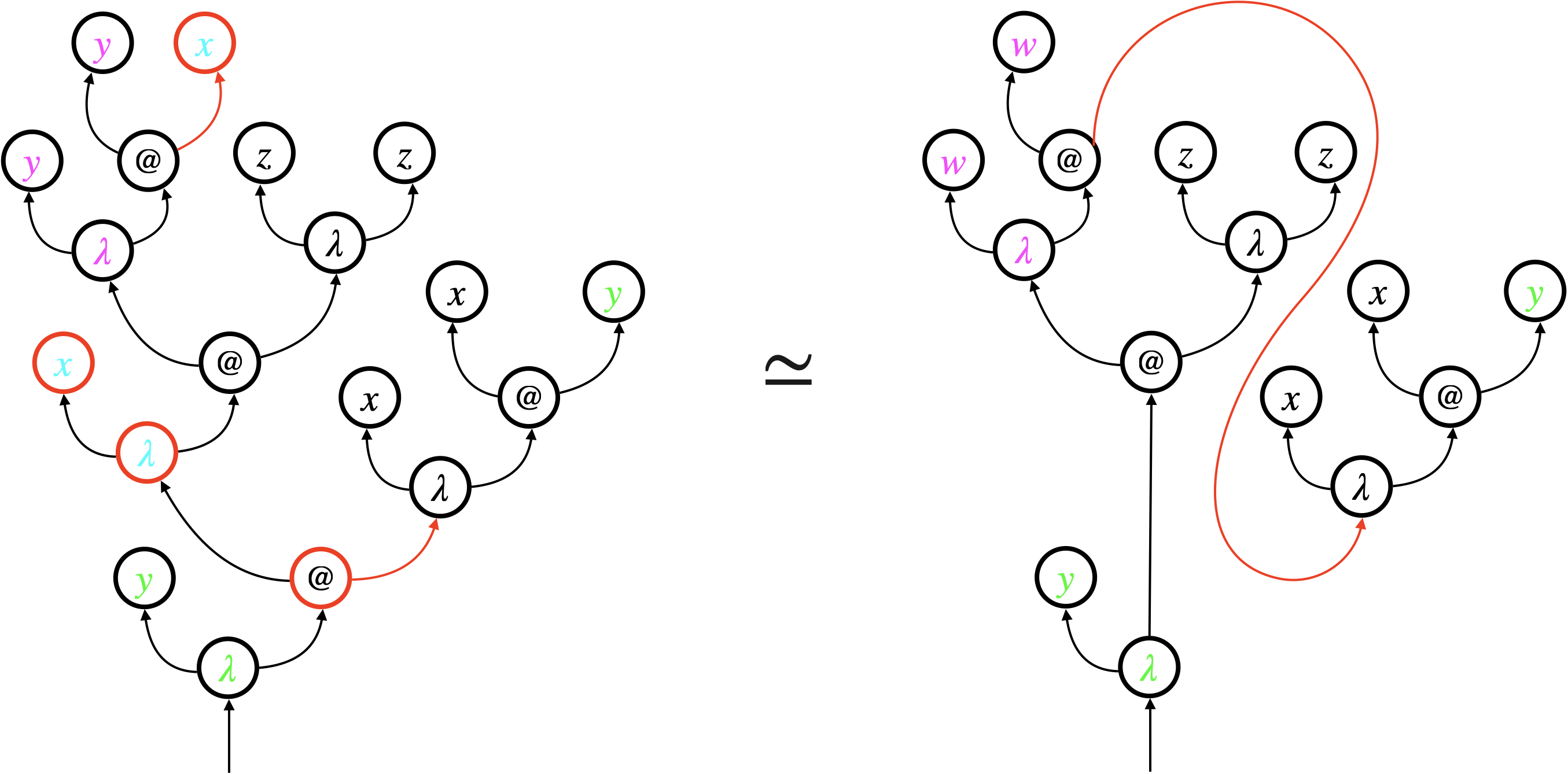
Figure 1a shows the beta-law (1) using ASTs. The scope of each variable is not obvious in the ASTs, which is why we keep using colours to distinguish variable scopes. The law deletes the four red nodes of the left AST, and connects two red arrows to represent substitution for . Additionally, all occurrences of the variable has to be renamed to .
We propose hypernets as an alternative graph representation. Hypernets, inspired by proof nets [Gir87], replace variable names with virtual connection, and hence keep variables anonymous. Binding structures and scopes are made explicit by (dashed) boxes around sub-graphs.
Figure 1b shows the same beta-law (1) using hypernets instead of ASTs. Each bound variable is simply represented by an arrow that points at the left edge of the associated dashed box. For example, the upper one of the two red arrows in the left hypernet represents the bound variable . It points at the left edge of the red dashed box that represents the scope of the variable. The dashed box is connected to the corresponding binder ().
The beta-law requires relatively local changes to hypernets. In Figure 1b, the two red nodes are deleted, the associated red dashed box is also deleted, and the two red arrows are connected to represent substitution for . There is no need for renaming , as it is simply represented by an anonymous arrow.
Remark 1 (Arrows representing bound variables).
In hypernets, the arrow representing a bound variable points at the left edge of the associated dashed box. In other graphical notations (e.g. proof nets [Gir87]), the bound variable would be connected to the corresponding binder (), as shown by red arrows in Figure 1c. We treat these red arrows as mere decorations, and exclude them from the formalisation of hypernets. We find that boxes suffice to delimit the scope of variables and sub-terms. Exclusion of decorations also simplifies the formalisation by reducing the number of loops in each hypernet. ∎
2.2. Focussed hypernet rewriting
The main difference between a law (an equation) and a reduction is that the former can be applied in any context, at any time, whereas the latter must be applied strategically, in a particular (evaluation) context and in a particular order. Different reduction strategies, for instance, make different programming languages out of the same calculus.
The question to be addressed here is how to define strategies for determining redexes in hypernets. Our operational semantics, i.e. focussed hypernet rewriting, combines graph traversal with update, and exploits the traversal to search for a redex.
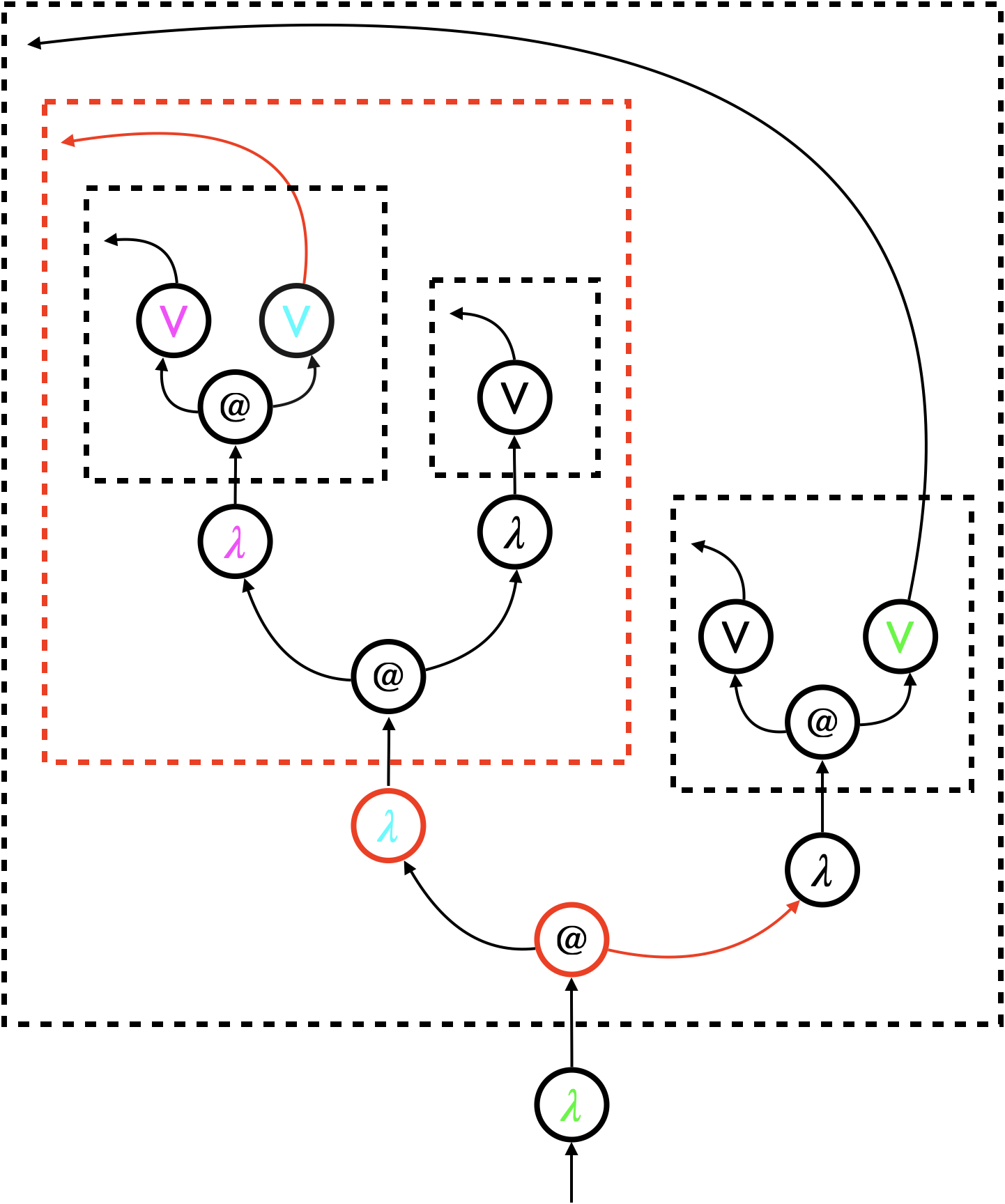
Let us illustrate focussed hypernet rewriting, using the call-by-value reduction of the linear lambda-term as shown in Figure 2. The thicker green arrows are not part of the hypernets but they show the traversal. The reduction proceeds as follows.
-
(1)
The depth-first traversal witnesses that the abstraction is a value, and that the sub-term contains two abstractions and it is ready for the beta-reduction. In the reduction, an application node () and its matching abstraction node () are deleted, and the associated dashed box is removed. The argument is then connected to the bound variable , yielding the second hypernet.
-
(2)
The traversal continues on the resultant hypernet (representing ), confirming that the result of the beta-reduction is a value. Note that the abstraction has already been inspected in the previous step, so the traversal does not repeat the inspection. It only witnesses the abstraction at this stage. The beta-reduction is then triggered, yielding the third and final hypernet representing .
-
(3)
The traversal confirms that the result of the beta-reduction is a value, and it finishes.
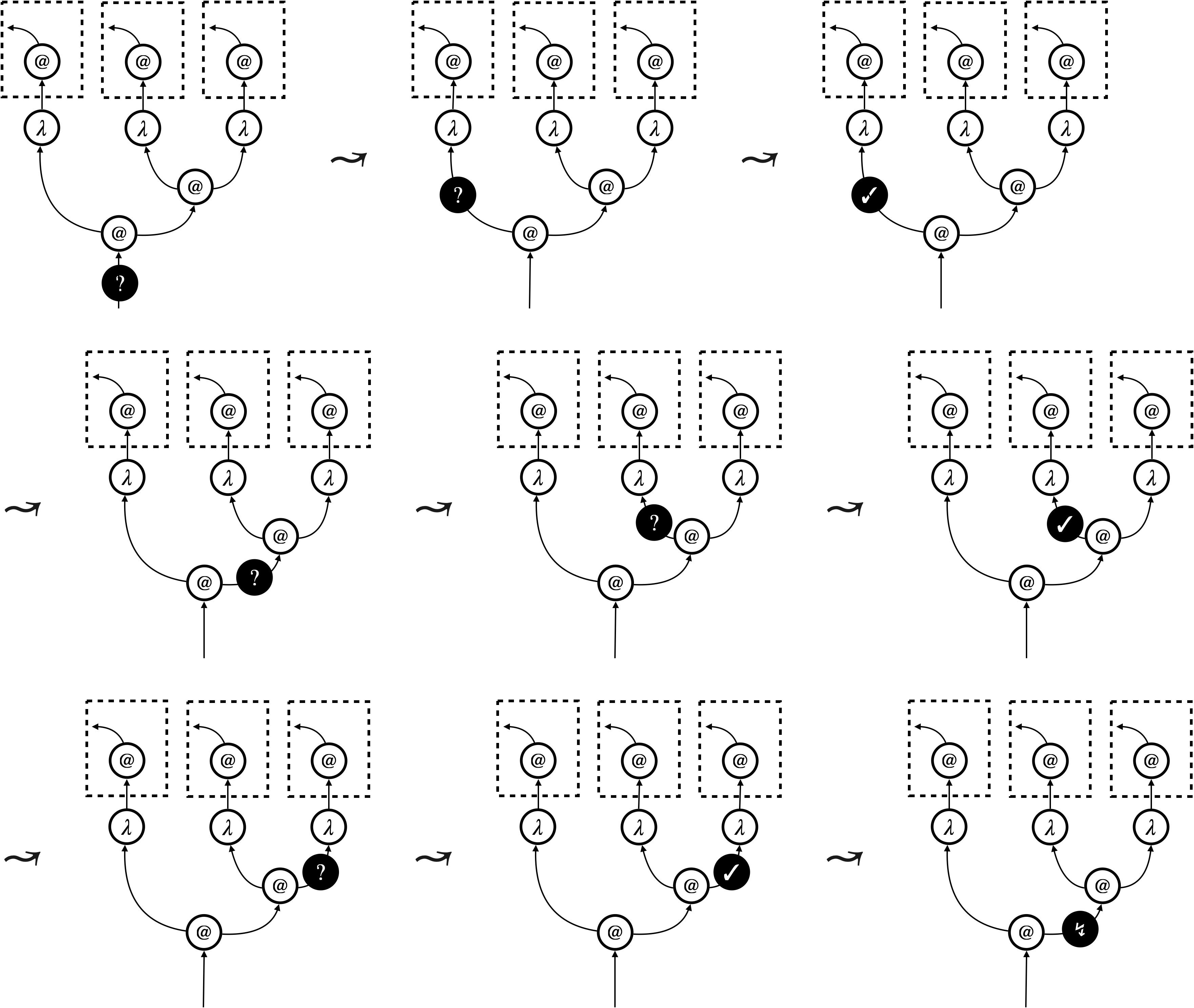
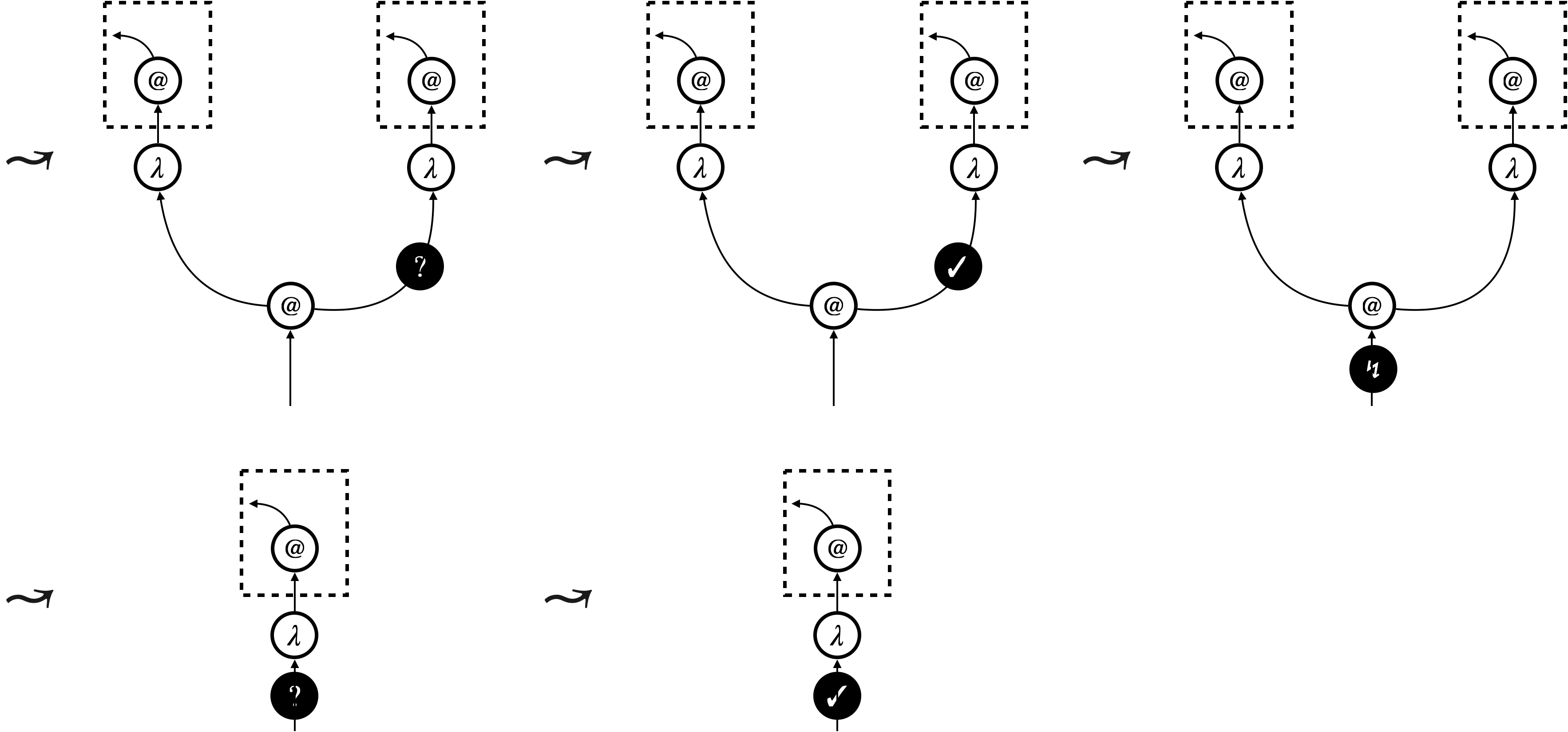
We implement focussed hypernet rewriting, in particular the graph traversal (the thick green arrows in Figure 2), using a dedicated node dubbed focus. A focus can be in three modes: searching (), backtracking (), and triggering (). The first two modes implement the depth-first traversal, and the last mode triggers update of the underlying hypernet. Figure 3 shows how focussed hypernet rewriting actually proceeds222An interpreter and visualiser can be accessed online at https://tnttodda.github.io/Spartan-Visualiser/, given the linear term . The black nodes are the focus. The first eight steps altogether implement the thick green arrow in the first part of Figure 2. At the end of these steps, the focus changes to , signalling that the hypernet is ready for the beta-reduction. What follows is an update of the hypernet, which resets the focus to the searching mode (), so the traversal continues and triggers further update.
Evaluation of a program starts, when the -focus enters the hypernet representing from the bottom. Evaluation successfully finishes, when the -focus exits a hypernet from the bottom.
We will formalise focussed hypernet rewriting as an abstract machine (see [Pit00] for a comprehensive introduction). The machine has two kinds of transitions: one for the traversal, and the other for the update. It is important that the focus governs transitions; a traversal transition or an update transition is selected according to the mode of the focus. It is the focus that implements the traversal, triggers the update, and hence realises the call-by-value reduction strategy.
2.3. Step-wise local reasoning, and robustness
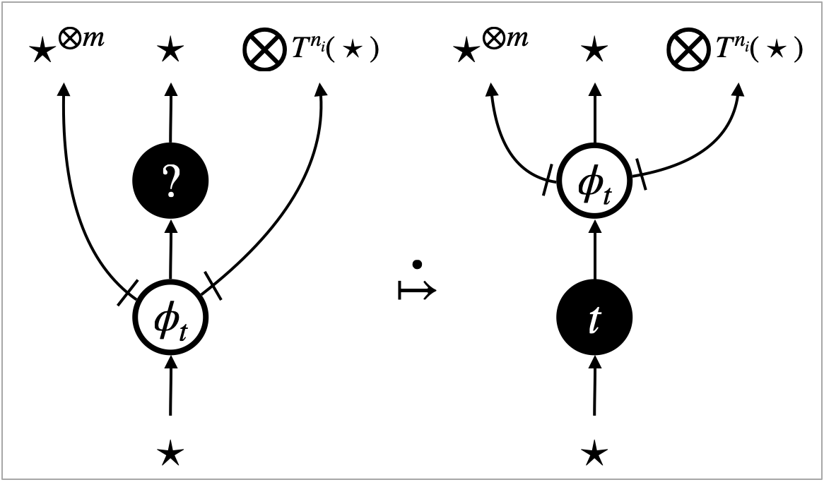
Finally we overview the reasoning principle that focussed hypernet rewriting enables, which leads to our main theorem, sufficiency-of-robustness theorem (6).
Using focussed hypernet semantics, this work takes a new coinductive, step-wise, approach to proving observational equivalence. We will introduce a new variant of weak simulation dubbed counting simulation. A counting simulation is a relation on focussed hypernets that are hypernets with a focus. We write to indicate that a hypernet contains a focus.
Our proof of an observational refinement , which is the asymmetric version of observational equivalence , proceeds as follows.
-
(1)
We start with the relation on hypernets. We call it pre-template.
-
(2)
We take the contextual closure of the pre-template . It is defined by for an arbitrary focussed (multi-hole) context .
-
(3)
We show that is a counting simulation.
Once we establish the counting simulation , soundness of counting simulation asserts that the pre-template implies observational refinement .
The key part of the observational refinement proof is therefore showing that is a counting simulation. Put simply, this amounts to show the following: for any and a transition , there exists a focussed context that satisfies the following.
| (2) |
Above, black parts are universally quantified, and magenta parts are existentially quantified. The arrow represents an arbitrary number of transitions . This situation (2) asserts that, after a few transitions from and , we can obtain two focussed hypernets that can be decomposed using the new context and the sub-graphs .
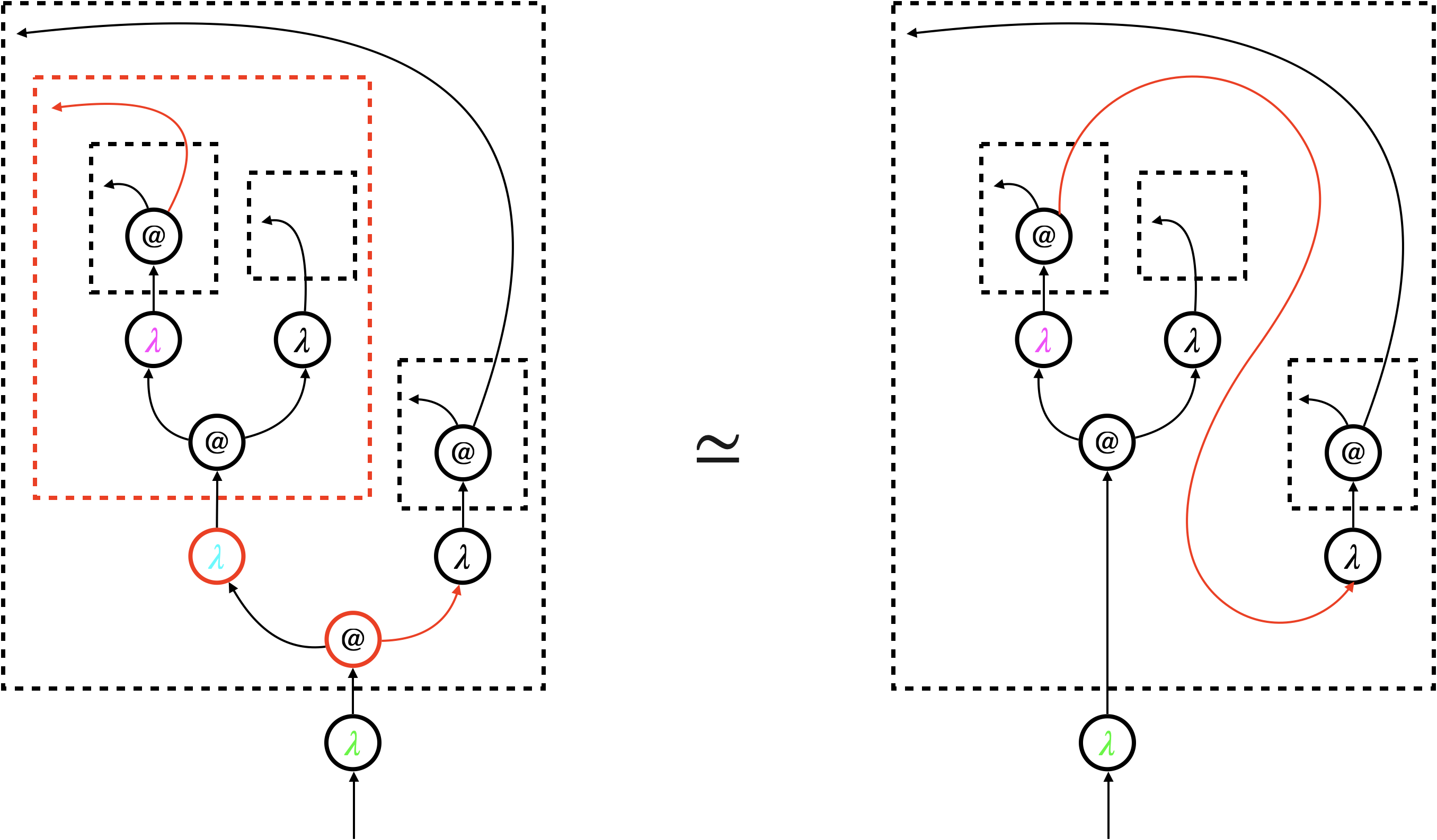
Our important observation is that (2) can be established by elementary case analysis of interaction between the sub-graphs and what happens around the focus in . This is because updates of a hypernet always happen around the -focus, and the -focus and the -focus (representing the graph traversal) move according to its neighbourhood. The analysis is hence centred around the graphical concept of neighbourhood, or graph locality. There are three possible cases of the interaction.
- Case (i) Move inside the context:
-
The -focus or the -focus, which implements the depth-first traversal, simply moves inside the context (see Figure 4a). Because any move of the focus is only according to its neighbourhood, the move solely depends on the context . In other words, the sub-graphs have no interaction with the focus. In this case, we can conclude that we are always in (2).
- Case (ii) Visit to the sub-graphs:
-
The -focus visits the sub-graphs (see Figure 4b). This is the case where the -focus actually interacts with ; what happens after entering of the focus depends on . We identify a sufficient condition of the pre-template , dubbed safety, for (2) to hold.
A typical example of safe pre-templates is the pre-templates that are induced by rewrite rules of hypernets. Figure 4c illustrates what happens to such a pre-template. The visit of the -focus to triggers the rewrite rule, and actually turns into .
Note that the case where the -focus visits boils down to the visit of the -focus instead, because the -focus implements backtracking of graph traversal.
- Case (iii) Update of the hypernets:
-
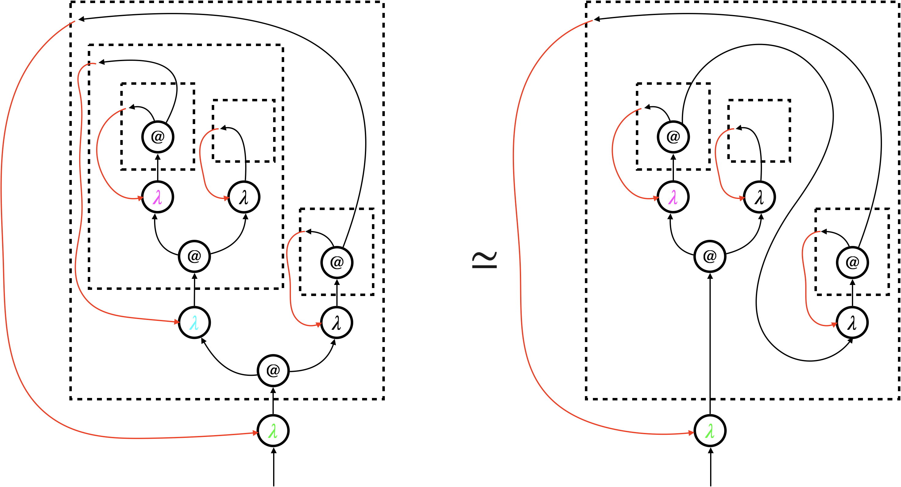
The -focus triggers a rewrite rule and updates the hypernet (see Figure 4d). This is the case where the -focus interacts with ; the update may involve in a non-trivial manner. We identify a sufficient condition of the pre-template , relative to the triggered rewrite rule, dubbed robustness, for (2) to hold.
An example scenario of robustness is where the update only affects parts of the context ; see Figure 4e. In this scenario, the -focus does not really interact with . The sub-graphs are preserved, and we can take the new context with the same number of holes as that makes (2) hold.
Another example scenario of robustness is where the update duplicates (or eliminates) without breaking them. We can take the context that has more (or less) holes to make (2) hold. ∎
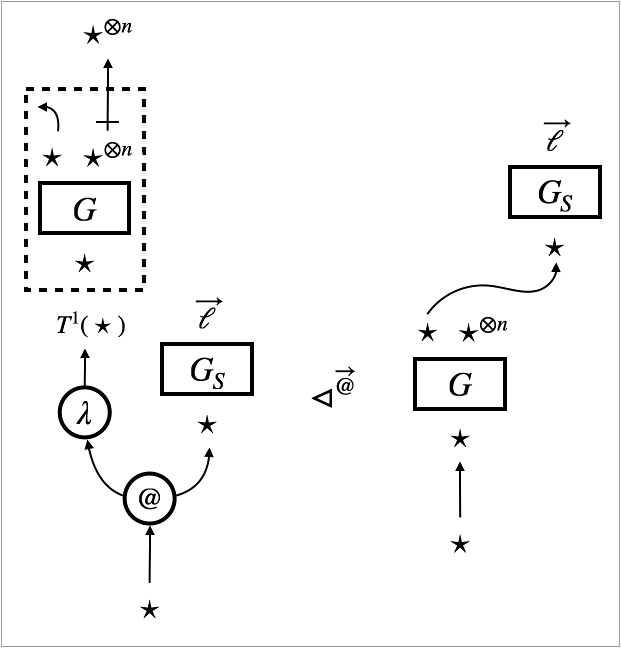
The above case analysis reveals sufficient conditions, namely safety and robustness, to make (2) hold and hence make the context closure a counting simulation. Combining this with soundness of counting simulation, we obtain our main theorem, sufficiency-of-robustness theorem (6). It can be informally stated as follows.
Theorem (Sufficiency-of-robustness theorem (6), informally).
A robust and safe pre-template induces observational refinement .
3. Preliminaries: Hypernets
We start formalising the ideas described in the previous section, by first defining hypernets. We opt for formalising hypernets as hypergraphs, following the literature [BGK+22a, BGK+22b, BGK+22c, AGSZ22] on categorically formalising string diagram rewriting using hypergraphs.
Let be the set of natural numbers. Given a set we write by the set of elements of the free monoid over . Given a function we write for the pointwise application (map) of to the elements of .
3.1. Monoidal hypergraphs and hypernets
Hypernets have a couple of distinctive features in comparison with ordinary graphs. The first feature of hypernets is that they have “dangling edges” (see Figure 1b); a hypernet has one incoming arrow with no source, and it may have outgoing arrows with no targets. To model this, we use hypergraphs—we formalise what we have been calling edges (i.e. arrows) as vertices and what we have been calling nodes (i.e. circled objects) as hyperedges (i.e. edges with arbitrary numbers of sources and targets). More specifically, we use what we call interfaced labelled monoidal hypergraphs that satisfies the following.
-
(0)
Each arrow (modelled as a vertex) and each circled object (modelled as a hyperedge) are labelled.
-
(1)
Each circled object (modelled as a hyperedge) is adjacent to distinct arrows (modelled as vertices).
-
(2)
Each arrow (modelled as a vertex) is adjacent to at most two circled objects (modelled as hyperedges).
-
(3)
The label of a circled object (modelled as a hyperedge) is always consistent with the number and labelling of its endpoints.
-
(4)
Dangling arrows are ordered, and each arrow has at least a source or a target.
[Monoidal hypergraphs] A monoidal hypergraph is a pair of finite sets, vertices and (hyper)edges along with a pair of functions , defining the source list and target list, respectively, of an edge. {defi}[Interfaced labelled monoidal hypergraphs] An interfaced labelled monoidal hypergraph consists of a monoidal hypergraph, a set of vertex labels , a set of edge labels , and labelling functions such that:
-
(1)
For any edge , its source list consists of distinct vertices, and its target list also consists of distinct vertices.
-
(2)
For any vertex there exists at most one edge such that and at most one edge such that .
-
(3)
For any edges if then , and .
-
(4)
If a vertex belongs to the target (resp. source) list of no edge we call it an input (resp. output). Inputs and outputs are respectively ordered, and no vertex is both an input and an output.
Notation 3.0 (Types of circled objects (i.e. hyperedges)).
Section 3.1 (3) makes it possible to use labels of arrows (i.e. vertices) as types for labels of circled objects (i.e. hyperedges). For each , we can associate it a type and write , where satisfy and for any such that .
Notation 3.0 (Types of interfaced labelled monoidal hypergraphs).
The concept of type can be extended to a whole interfaced labelled monoidal hypergraph . Let be the lists of inputs and outputs, respectively, of . We associate a type and write . In the syntax for lists of inputs and outputs we use to denote concatenation and define to be the empty list, and , for any label and .
In the sequel, when we say hypergraphs we always mean interfaced labelled monoidal hypergraphs.
We sometimes permute inputs and outputs of a hypergraph. Such permutation yields another hypergraph. {defi}[Interface permutation] Let be a hypergraph with an input list and an output list . Given two bijections and on sets and , respectively, we write to denote the hypergraph that is defined by the same data as except for the input list and the output list .
The second distinctive feature of hypernets is that they have dashed boxes that indicate the scope of variable bindings (see Figure 1b). We formalise these dashed boxes by introducing hierarchy to hypergraphs. The hierarchy is implemented by allowing a hypergraph to be the label of a hyperedge. As a result, informally, hypernets are nested hypergraphs, up to some finite depth, using the same sets of labels. We here present a relatively intuitive definition of hypernets; Appendix A discusses an alternative definition of hypernets333Another, slightly different, definition of hypernets is given in [AGSZ23, Section 4]. The difference is motivated by desired support of categorical graph rewriting, which requires certain properties to hold. These properties are sensitive to the definition.. {defi}[Hypernets] Given a set of vertex labels and edge labels we write for the set of hypergraphs with these labels; we also call these level-0 hypernets . We call level- hypernets the set of hypergraphs
We call hypernets the set .
Terminology 3.0 (Boxes and depth).
An edge labelled with a hypergraph is called box edge, and a hypergraph labelling a box edge is called content. Edges of a hypernet are said to be shallow. Edges of nesting hypernets of , i.e. edges of hypernets that recursively appear as edge labels, are said to be deep edges of . Shallow edges and deep edges of a hypernet are altogether referred to as edges at any depth.
3.2. Graphical conventions

A hypergraph with vertices and edges such that
is normally represented as Figure 5a. However, we find this style of representing hypergraphs awkward for understanding their structure. We will often graphically represent hypergraphs as graphs, as in Figure 5b, by (i) marking vertices with their labels and mark hyperedges with their labels circled, and (ii) connecting input vertices and output vertices with a hyperedge using arrows.
Recall that node labels are often determined in hypergraphs, thanks to typing, e.g. . We accordingly omit node labels to avoid clutter, as in Figure 5c, letting arrows connect circles directly.
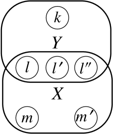
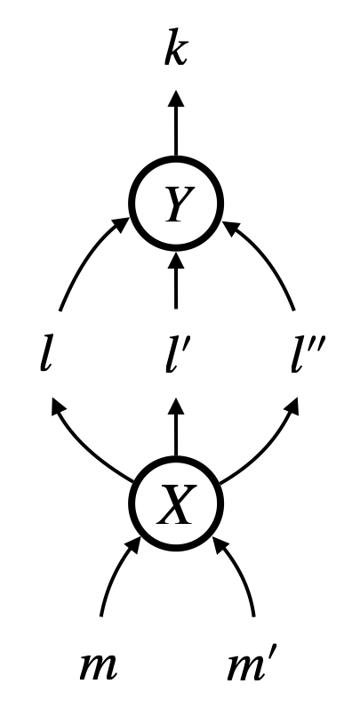
Sometimes we draw a hypergraph by connecting its sub-graphs using extra arrows. Sub-graphs are depicted as boxes. For the hypergraph , we can think of the sub-graph and the sub-graph . We may draw in three ways, as in Figure 5d–5f:
-
•
In Figure 5d, we use extra arrows connecting node labels directly, with intention that two occurrences of (or, ) are graphical representations of the same node (or ).
-
•
In Figure 5e, we omit node labels entirely, assuming that they are obvious from context.
-
•
In Figure 5f, we further replace the three extra arrows with a single arrow, given that the entire output type of matches the input type of . The single arrow comes with a dash across, which indicates that the arrow represents a bunch of parallel arrows.
The final convention is about box edges; a box edge (i.e. an edge labelled by a hypernet) is depicted by a dashed box decorated with its content (i.e. the labelling hypernet).
4. Representation of the call-by-value untyped linear lambda-calculus
In this section we introduce specific label sets that we use to represent lambda-terms as hypernets. We begin with the untyped linear lambda-calculus extended with arithmetic. This is a fairly limited language in terms of expressive power. Although simple, it is interesting enough to demonstrate our reasoning framework. We present a translation of linear lambda-terms in this section, and will adapt it to the general lambda-terms in Section 9.
Lambda-terms are defined by the BNF , where and . We assume alpha-equivalence on terms, and assume that bound variables are distinct in a term. A term is linear when each variable appears exactly once in .
First, recall that each edge label of a hypernet comes with a type where . Even though lambda-terms are untyped here, we use edges to represent term constructors, and use edge types (i.e. node labels) to distinguish thunks from terms. Namely, the term type is denoted by , and a thunk type with bound variables is denoted by .
Figure 6 shows inductive translation of linear lambda-terms to hypernets where
| (3) | ||||
| (4) |
In general, a term with free variables is translated into . Each term constructor is turned into an edge as follows.
-
•
Any variable becomes an anonymous edge . We represented a variable as a single arrow in Section 2 (see e.g. Figure 1b and Figure 3), but this means a variable would become an empty graph (i.e. a hypernet with no edge). We rather use the anonymous edge to prevent an empty graph from labelling a box edge and hence being a box content. This is for technical reasons as they simplify our development.
-
•
Abstraction becomes ; it constructs a term, taking one thunk that has one bound variable. A thunk that has one bound variable and free variables is represented by a box edge of type whose content is . Note that the box has one less output than its content. We emphasise this graphically, by bending the arrow that is connected to the leftmost of the type .
-
•
Application becomes ; it constructs a term, taking two terms as arguments. This translation is for the call-by-value evaluation strategy; both of the arguments are not thunks, and hence they will be evaluated before the application is computed.
-
•
Each natural number becomes ; it is a term, taking no arguments.
-
•
Arithmetic operations becomes and ; they construct a term, taking two terms as arguments. The translation for these operations has the same shape as that for application.
5. Focussed hypernet rewriting—the Universal Abstract Machine
In this section we present focussed hypernet rewriting. It will be formalised as an abstract machine dubbed universal abstract machine (UAM). This abstract machine is “universal” in a sense of the word similar to the way it is used in “universal algebra” rather than in “universal Turing machine”. It is a general abstract framework in which a very wide range of concrete abstract machines can be instantiated by providing operations and their behaviour.
5.1. Operations and focus
The first parameter of the UAM is given by a set of operations . Operations are classified into two: passive operations that construct evaluation results (i.e. values) and active operations that realise computation. We let range over respectively. The edge labels in (4), except for , are examples of operations:
| passive operations | active operations |
|---|---|
| for each | where |
In general, each operation has a type where . This means that each operation takes arguments and thunks, and the -th thunk has bound variables.
Given the operation set , the UAM acts on hypernets where
| (5) |
We let range over . For box edges, we impose the following type discipline: each box edge must have a type with its content having a type .
The last three elements of (5) are focuses. In the UAM, focuses are edges with the dedicated labels of type . Each label represents one of the three modes of the focus:
| label | mode |
|---|---|
| searching | |
| backtracking | |
| triggering an update |
As illustrated in Section 2.2, focussed hypernet rewriting implements program evaluation by combining (i) depth-first graph traversal and (ii) update (rewrite) of a hypernet. Focuses are the key element of this combination; they determine which action (i.e. traversal or rewrite) to be taken next, and they indicate where a redex of the rewrite is.
We refer to a hypernet that contains one focus as focussed hypernet. Given a focussed hypernet, we refer to the hypernet without the focus as underlying hypernet.
5.2. Transitions—overview
| transitions | focus | provenance | |
|---|---|---|---|
| search transitions | intrinsic | ||
| rewrite transitions | substitution transitions | ||
| behaviour | extrinsic | ||
| (compute transitions) | |||
Table 1 summarises classifications of transitions of the UAM.
The first classification is according to the focuses: search transitions for the -focus and the -focus, implementing the depth-first search of redexes, and rewrite transitions for the -focus, implementing rewrite of the underlying hypernet. Rewrite transitions are further classified into two: substitution transitions for edges labelled by , and behaviour for (active) operations.
The next classification is according to provenance: intrinsic transitions that are inherent to the UAM, and extrinsic transitions that are not. While search transitions and substitution transitions constitute intrinsic transitions, the behaviour solely provides extrinsic transitions. In fact, the behaviour is the second parameter of the UAM.
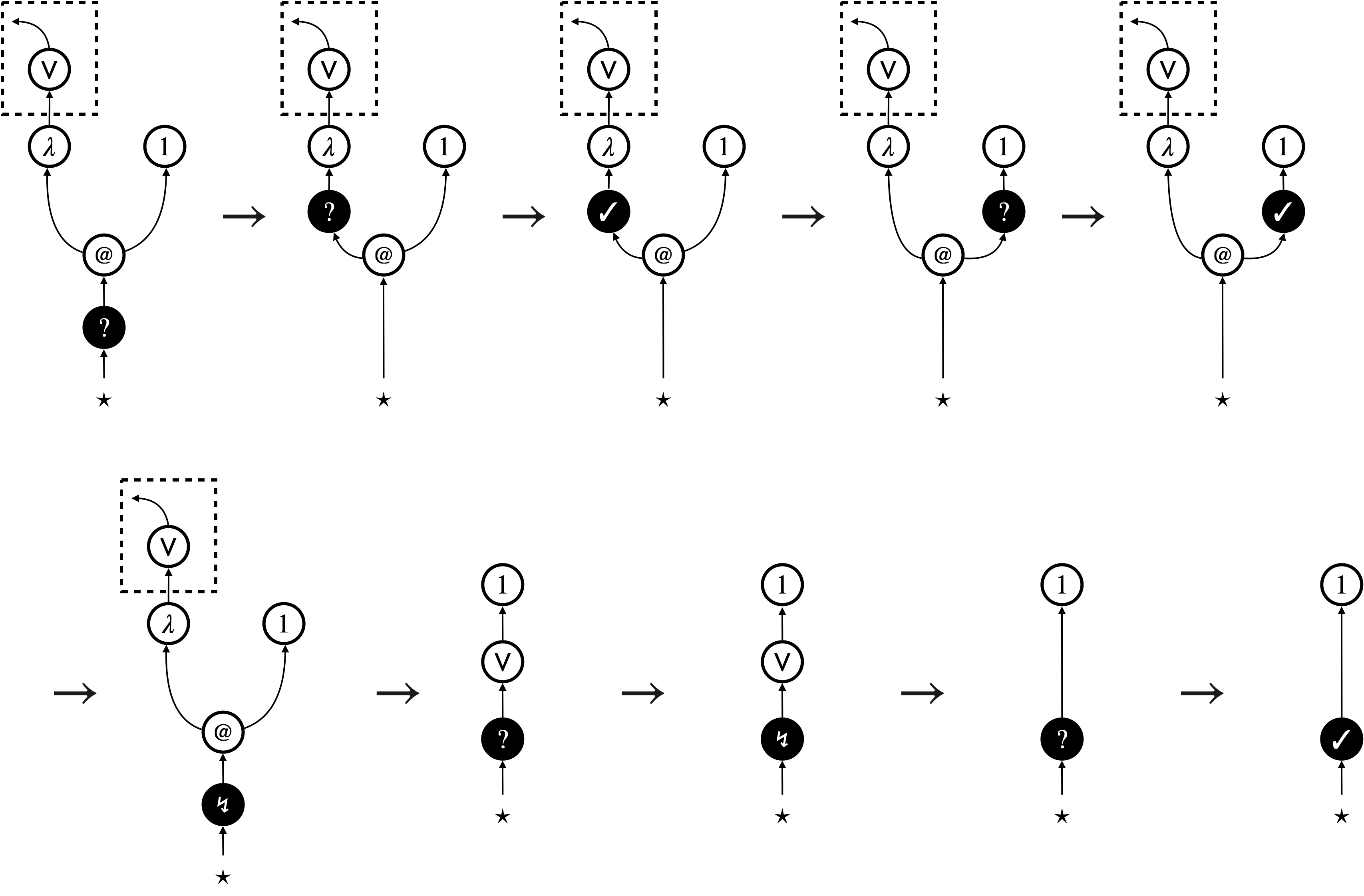
Figure 8 shows an example of the UAM execution. This evaluates the linear-term , and the execution starts with the underlying hypernet . It demonstrates all the three kinds of transitions: search transitions, substitution transitions, and the behaviour of application ().
5.3. Intrinsic transitions
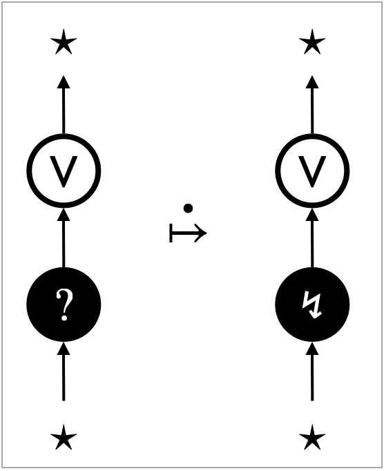
Search transitions are possible for the -focus and the -focus, and they implement the depth-first search of redexes. They are specified by interaction rules depicted in Figure 9a–9e. The -focus interacts with what is connected above, and the -focus interacts with what is connected below. From the perspective of program evaluation, the interaction rules specify the left-to-right call-by-value evaluation of arguments.
- Figure 9a:
-
When the -focus encounters a variable (), it changes to the -focus. What is connected above the variable will be substituted for the variable, in a subsequent substitute transition.
- Figure 9b:
-
When the -focus encounters an operation with at least one argument, it proceeds to the first argument.
- Figure 9c:
-
After inspecting the -th argument, the -focus changes to the -focus and proceeds to the next argument.
- Figure 9d:
-
After inspecting all the arguments, the -focus finishes redex search and changes to a focus depending on the operation : to the -focus for a passive operation , and to the -focus for an active operation .
- Figure 9e:
-
When the -focus encounters an operation that takes no arguments but only thunks, it immediately finishes redex search and changes to a focus depending on the operation , like in Figure 9d.
The first kind of rewrite transitions, namely substitution transitions, implements substitution by simply removing a variable edge (). These transitions are specified by a substitution rule depicted in Figure 9f. What is connected above the variable edge () is computation bound to the variable. By removing the variable edge, the bound computation gets directly connected to the -focus, ready for redex search.
5.4. Extrinsic transitions: behaviour of operations
The second kind of rewrite transitions are for operations , in particular active operations . These transitions are extrinsic; they are given as the second parameter , called behaviour of , of the UAM.
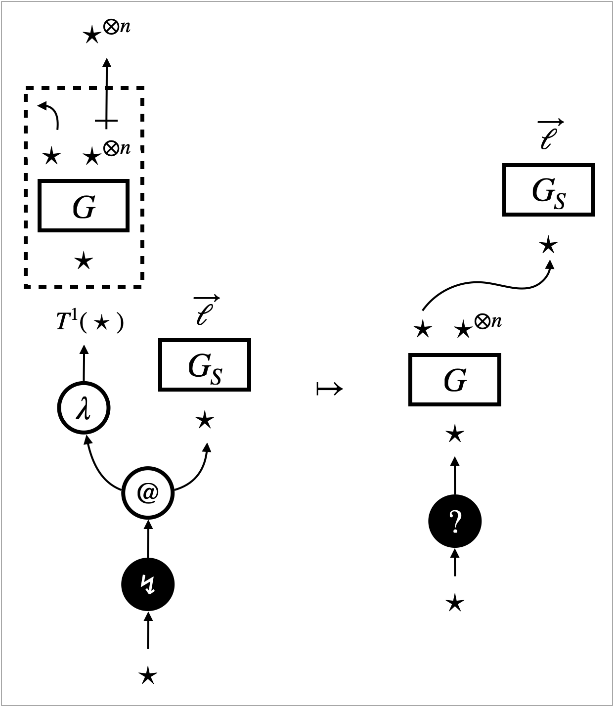
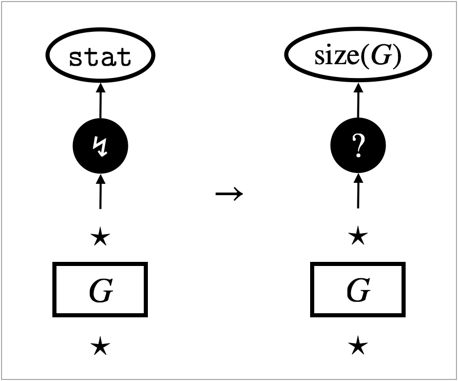
Figure 10 shows an example of the behaviour, namely that for the following active operations:
For some of these operations, their behaviour is specified locally by rewrite rules. The rewrite transitions for the four active operations are enabled when the -focus encounters one of the operations. The -focus then changes to the -focus and resumes redex search.
- Figure 10a:
-
This rewrite rule specifies the behaviour of arithmetic (). The rule eliminates all three edges () and replace them with a new edge () such that .
- Figure 10b:
-
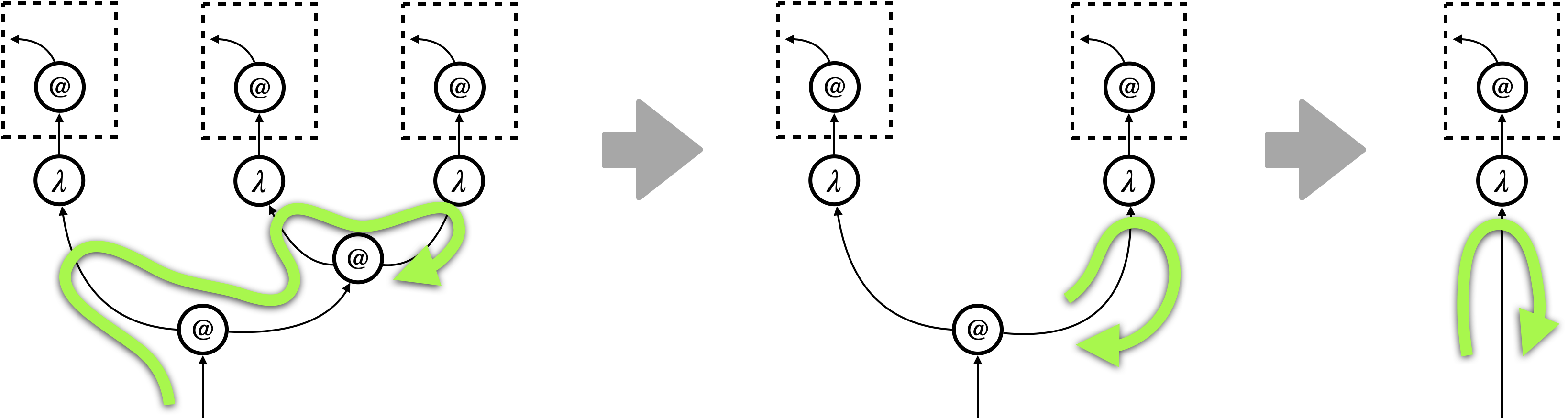
This rewrite rule specifies the behaviour of application (), namely the (micro-) beta-reduction. It is micro in the sense that it delays substitution. It only eliminates the constructors (), opens the box whose content is , and connects which represents a function argument to the body of the function.
- Figure 10c:
-
This is a rewrite transition, not a rewrite rule. It is for the operation that inspects memory usage. Namely, counts the number of edges in the hypernet . The transition replaces the operation edge () with the result () of counting.
6. A formal definition of the UAM
The UAM, and hence the definitions below, are all globally parameterised by the operation set and its behaviour .
6.1. Auxiliary definitions
We use the terms incoming and outgoing to characterise the incidence relation between neighbouring edges. Conventionally incidence is defined relative to nodes, but we find it helpful to extend this notion to edges. {defi}[Incoming and outgoing edges] An incoming edge of an edge has a target that is a source of the edge . An outgoing edge of the edge has a source that is a target of the edge .
The notions of path and reachability are standard. Our technical development will heavily rely on these graph-theoretic notions. Note that these are the notions that are difficult to translate back into the language of terms. {defi}[Paths and reachability]
-
(1)
A path in a hypergraph is given by a non-empty sequence of edges, where an edge is followed by an edge if the edge is an incoming edge of the edge .
-
(2)
A vertex is reachable from a vertex if holds, or there exists a path from the vertex to the vertex .
Note that, in general, the first edge (resp. the last edge) of a path may have no source (resp. target). A path is said to be from a vertex , if is a source of the first edge of the path. Similarly, a path is said to be to a vertex , if is a target of the last edge of the path. A hypergraph is itself said to be a path, if all edges of comprise a path from an input (if any) and an output (if any) and every vertex is an endpoint of an edge.
During focussed hypernet rewriting, operations are the only edges that the -focus can “leave behind”. The -focus is always at the end of an operation path. {defi}[Operation paths] A path whose edges are all labelled with operations is called operation path.
We shall introduce a few classes of hypernets below. The first is box hypernets that are simply single box edges. {defi}[Box hypernets] If a hypernet is a path of only one box edge, it is called box hypernet. The second is stable hypernets, in which a focus can never trigger a rewrite (i.e. a focus never changes to the -focus). Stable hypernets can be seen as a graph-based notion of values/normal form. For example, the hypernet that consists of an abstraction edge () only is a stable hypernet. {defi}[Stable hypernets] A stable hypernet is a hypernet , such that and each vertex is reachable from the unique input. The last is one-way hypernets, which will play an important role in local reasoning. These specify sub-graphs to which a focus enters only from the bottom (i.e. the -focus through an input), never from the top (i.e. the -focus through an output). Should the -focus enter from the top, it must have traversed upwards the sub-graph and left an operation path behind. One-way hypernets are defined by ruling out such operation paths. {defi}[One-way hypernets] A hypernet is one-way if, for any pair of an input and an output of such that and both have type , any path from to is not an operation path. For example, the underlying hypernet of the left hand side of the micro-beta rewrite rule (Figure 10b) is a one-way hypernet, if is stable. Should the -focus enters to from the top, it must be backtracking the depth-first search, and hence the -focus must have been visited from the bottom. In the presence of the micro-beta rewrite rule, such visit must result in a rewrite transition, and therefore, the backtracking of the -focus cannot be possible.
6.2. Focussed hypernets
Focussed hypernets are those that contain a focus. We impose some extra conditions as below, to ensure that the focus is outside a box and not isolated. {defi}[Focussed hypernets]
-
(1)
A focus in a hypergraph is said to be exposed if its source is an input and its target is an output, and self-acyclic if its source and its target are different vertices.
-
(2)
Focussed hypernets (typically ranged over by ) are those that contain only one focus and the focus is shallow, self-acyclic and not exposed.
Focus-free hypernets are given by , i.e. hypernets without a focus.
Notation 6.0 (Removing, replacing and attaching a focus).
-
(1)
A focussed hypernet can be turned into an underlying focus-free hypernet with the same type, by removing its unique focus and identifying the source and the target of the focus.
-
(2)
When a focussed hypernet has a -focus, then changing the focus label to another one yields a focussed hypernet denoted by .
-
(3)
Given a focus-free hypernet , a focussed hypernet with the same type can be yielded by connecting a -focus to the -th input of if the input has type . Similarly, a focussed hypernet with the same type can be yielded by connecting a -focus to the -th output of if the output has type . If it is not ambiguous, we omit the index in the notation .
The source (resp. target) of a focus is called “focus source” (resp. “focus target”) in short.
6.3. Contexts
We next formalise a notion of context, which is hypernets with holes. We use a set of hole labels, and contexts are allowed to contain an arbitrary number of holes. Hole labels are typed, and typically ranged over by . {defi}[(Simple) contexts]
-
(1)
Holed hypernets (typically ranged over by ) are given by , where the edge label set is extended by the set .
-
(2)
A holed hypernet is said to be context if each hole label appears at most once (at any depth) in .
-
(3)
A simple context is a context that contains a single hole, which is shallow.
By what we call plugging, we can replace a hole of a context with a hypernet, and obtain a new context. We here provide a description of plugging and fix a notation. A formal definition of plugging can be found in Appendix B.
Notation 6.0 (Plugging of contexts).
-
(1)
When gives a list of all and only hole labels that appear in a context , the context can also be written as . A hypernet in can be seen as a context without a hole and written as .
-
(2)
Let and be contexts, such that the hole and the latter context have the same type and . A new context can be obtained by plugging into : namely, by replacing the (possibly deep) hole edge of that has label with the context , and by identifying each input (resp. output) of with its corresponding source (resp. target) of the hole edge.
Each edge of the new context is inherited from either or , keeping the type; this implies that the new context is indeed a context with hole labels . Inputs and outputs of the new context coincide with those of the original context , and hence these two contexts have the same type.
The plugging is associative in two senses: plugging two contexts into two holes of a context yields the same result regardless of the order, i.e. is well-defined; and nested plugging yields the same result regardless of the order, i.e. .
The notions of focussed and focus-free hypernets can be naturally extended to contexts. We use the terms entering and exiting to refer to a focus that is adjacent to a hole. A focus may be both entering and exiting. {defi}[Entering/exiting focuses] In a focussed context , the focus is said to be entering if it is an incoming edge of a hole, and exiting if it is an outgoing edge of a hole.
6.4. States and transitions
We now define the UAM as a state transition system. States are hypernets that represent closed terms and hence have type . {defi}[States]
-
(1)
A state is given by a focussed hypernet of type .
-
(2)
A state is called initial if , and final if .
The following will be apparent once transitions are defined: initial states are indeed initial in the sense that no search transition results in an initial state; and final states are indeed final in the sense that no transition is possible from a final state.
Intrinsic transitions, which consists of search transitions and substitution transitions, are specified by the interaction rules and the substitution rule in Figure 9. Each intrinsic transition applies a rule outside a box and at one place. {defi}[Intrinsic transitions]
-
(1)
For each interaction rule , if there exists a focus-free simple context such that and are states, is a search transition.
-
(2)
For each substitution rule , if there exists a focus-free simple context such that and are states, is a substitution transition.
When a sequence of transitions consists of search transitions only, it is annotated by the symbol as .
Extrinsic transitions must have a specific form; namely they must be a compute transition. {defi}[Compute transitions] A transition is a compute transition if: (i) the first state has the -focus that is an incoming edge of an active operation edge; and (ii) the second state has the -focus. We can observe that substitution transitions or compute transitions are possible if and only if a state has the -focus, and they always change the focus to the -focus. We refer to substitution transitions and compute transitions altogether as rewrite transitions (cf. Table 1).
Compute transitions may be specified locally, by rewrite rules, in the same manner as the intrinsic transitions. Figure 10a & 10b shows examples of rewrite rules. We leave it entirely open what the actual rewrite associated to some operation is, by having the behaviour as parameter of the UAM as well as the operation set . This is part of the semantic flexibility of our framework. We do not specify a meta-language for encoding effects as particular transitions. Any algorithmic state transformation (e.g. the compute transition for in Figure 10c) is acceptable.
We can now define the UAM as follows. {defi}[the UAM] Given two parameters and , the universal abstract machine (UAM) is given by data such that:
-
•
is a set of states,
-
•
is a set of intrinsic transitions, and
-
•
is a set of compute transitions.
We refer to elements of as extrinsic transitions, as well as compute transitions; we use these two terms interchangeably.
An execution of the UAM starts with a focus-free hypernet that represents a closed term, e.g. a result of the translation (cf. Figure 6). It is successful if it terminates with a final state, and not if it gets stuck with a non-final state. {defi}[Execution and stuck states]
-
(1)
An execution on a focus-free hypernet is a sequence of transitions starting from the initial state .
-
(2)
A state is said to be stuck if it is not final and cannot be followed by any transition.
Recall that we have a notion of stable hypernet (Section 6.1) that is a graphical counterpart of values. An execution on any stable hypernet terminates successfully at a final state, with only search transitions (cf. 33(1) which is proved for the “non-linear” UAM).
7. Contextual equivalence on hypernets
In this section, we set the target of our proof methodology. First, we define contextual equivalence in a general manner. Next, we clarify what kind of operations our proof methodology applies to.
7.1. Generalised contextual equivalence
We propose notions of contextual refinement and equivalence that check for successful termination of execution444We opt for the very basic notion of contextual refinement that concerns termination only. Richer observation (e.g. evaluation results, output, probability, nondeterminism) would require different definitions of contextual refinement, and these are out of the scope of this paper. . Our notion of contextual refinement (and hence contextual equivalence) generalise the standard notions in two ways.
-
•
The notion of contextual refinement can be flexible in terms of a class of contexts in which it holds. Namely, contextual refinement is parameterised by a set of focus-free contexts. The standard contextual refinement can be recovered by setting to be the set of all focus-free contexts.
-
•
The notion of contextual refinement can count and compare the number of transitions. Namely, contextual refinement is parameterised by a preorder on natural numbers. The standard contextual refinement can be obtained by setting to be the total relation . Other typical examples of the preorder are the greater-than-or-equal relation and the equality . With these preorders, one can prove that two terms are contextually equivalent, and moreover, one takes a less number of transitions to terminate than the other (with ) or the two terms take exactly the same number of transitions to terminate (with ).
We require the parameter to be closed under plugging, i.e. for any contexts such that is defined, . {defi}[State refinement and equivalence] Let be a preorder on , and and be two states.
-
•
is said to refine up to , written as , if for any number and any final state such that , there exist a number and a final state such that and .
-
•
and are said to be equivalent up to , written as , if and .
[Contextual refinement and equivalence] Let be a set of contexts that is closed under plugging, be a preorder on , and and be focus-free hypernets of the same type.
-
•
is said to contextually refine in up to , written as , if any focus-free context , such that and are states, yields refinement .
-
•
and are said to be contextually equivalent in up to , written as , if and .
In the sequel, we simply write etc., making the parameter implicit.
Because is a preorder, and are indeed preorders, and accordingly, equivalences and are indeed equivalences (35).
When the relation is the universal relation , the notions concern successful termination, and the number of transitions is irrelevant. If all compute transitions are deterministic, contextual equivalences and coincide for any (as a consequence of 36).
Because is closed under plugging, the contextual notions and indeed become congruences. Namely, for any and such that and are defined, , where .
As the parameter , we will use the set of all focus-free contexts, for the time being. We will use another set in Section 11. The standard notions of contextual refinement and equivalence can be recovered as and .
7.2. Determinism and refocusing
We will focus on operations whose behaviour makes the UAM both deterministic and refocusing in the following sense. {defi}[Determinism and refocusing]
-
(1)
A UAM is deterministic if the following holds: if two transitions and are possible, it holds that up to graph isomorphism.
-
(2)
A state is rooted if .
-
(3)
A UAM is refocusing if every transition preserves the rooted property.
In a refocusing UAM, the rooted property becomes an invariant, because any initial state is trivially rooted. The invariant ensures the following: starting the search process (i.e. a search transition) from a state with the -focus can be seen as resuming the search process , from an initial state, on the underlying hypernet . Resuming redex search after a rewrite, rather than starting from scratch, is an important aspect of abstract machines. In the case of the lambda-calculus, enabling the resumption is identified as one of the key steps (called “refocusing”) to synthesise abstract machines from reduction semantics by Danvy et al. [DMMZ12]. In our setting, it is preservation of the rooted property that justifies the resumption.
For many rewrite transitions that are specified by a local rewrite rule, it suffices to check the shape of the rewrite rule, in order to conclude that the corresponding rewrite transition preserves the rooted property. Intuitively, a rewrite rule (or the substitution rule) should satisfy the following.
-
(1)
No -focus can encounter prior to application of the rewrite rule .
-
(2)
The rewrite rule changes only edges above the -focus, and turns the focus into the -focus without moving it around.
-
(3)
If the -focus encounters , subsequent search transitions yield the -focus.
The above idea is formalised as a notion of stationary rewrite transition. If a rewrite transition is stationary in the following sense, it preserves the rooted property. {defi}[Stationary rewrite transitions] A rewrite transition is stationary if there exist a focus-free simple context , focus-free hypernets and , and a number , such that the following holds.
-
(1)
is one-way,
-
(2)
and , and
-
(3)
for any , such that is a state, there exists a state with the -focus, such that .
Lemma 2 (27).
If a rewrite transition is stationary, it preserves the rooted property, i.e. being rooted implies is also rooted.
Finally, determinism and refocusing of a UAM boil down to those of extrinsic transitions under a mild condition.
Lemma 3 (Determinism and refocusing).
-
•
A universal abstract machine is deterministic if extrinsic transitions are deterministic.
-
•
Suppose that in the substitution rule (Figure 9f) is a stable hypernet. A universal abstract machine is refocusing if extrinsic transitions preserve the rooted property.
Proof 7.1.
Intrinsic transitions and extrinsic transitions are mutually exclusive, and intrinsic transitions are all deterministic for the following reasons.
-
•
Search transitions are deterministic, because at most one interaction rule can be applied at any state.
-
•
Although two different substitution rules may be possible at a state, substitution transitions are still deterministic. Namely, if two different substitution rules and can be applied to the same state, i.e. there exist focus-free simple contexts and such that , then these two rules yield the same transition, by satisfying .
Therefore, if extrinsic transitions are deterministic, all transitions become deterministic.
Search transitions trivially preserve the rooted property. Substitution transitions also preserve the rooted property, because they are stationary, under the assumption that in Figure 9f is stable. Therefore, all transitions but extrinsic transitions already preserve the rooted property.
8. A sufficiency-of-robustness theorem
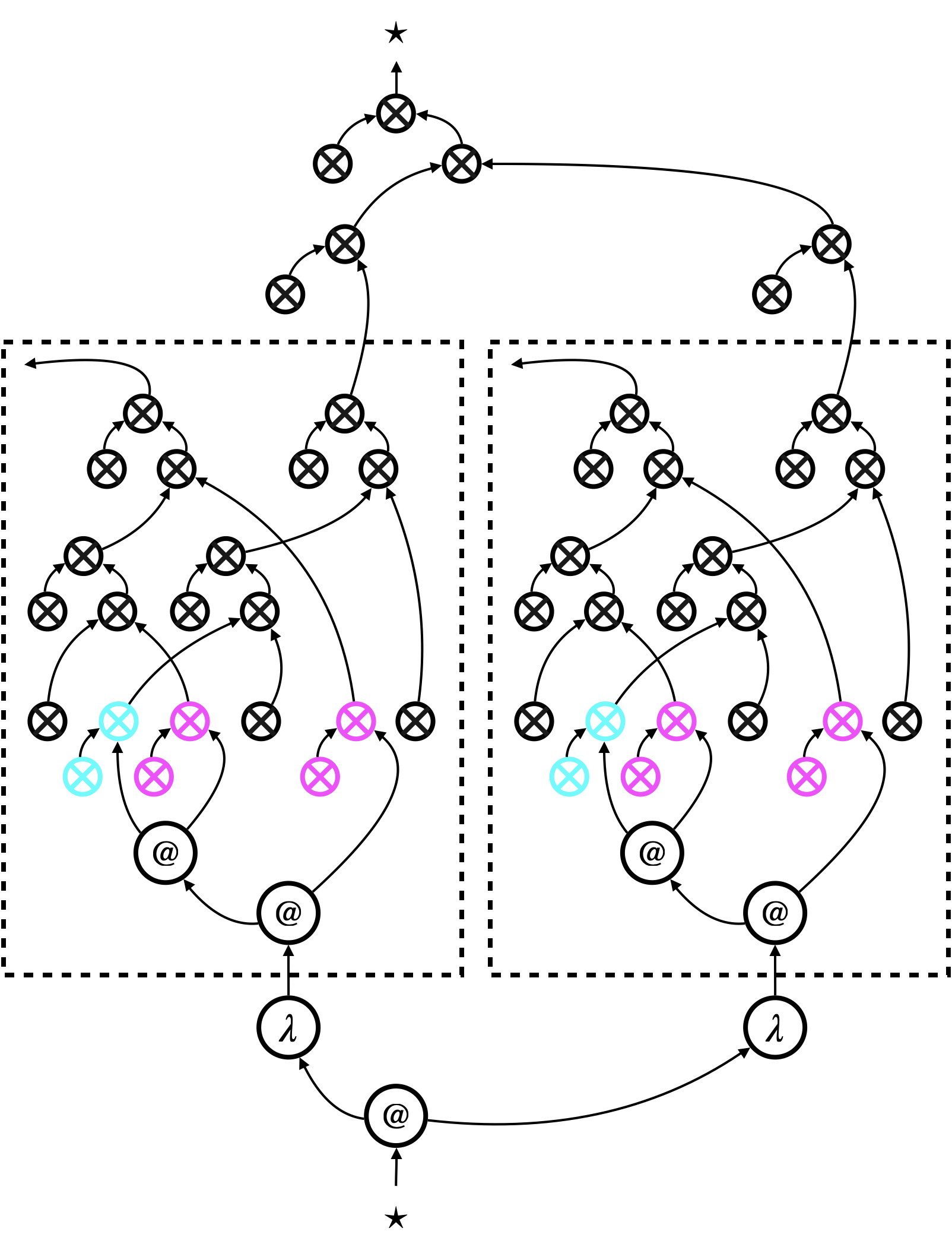
In this section, we will state a sufficiency-of-robustness theorem (6), by identifying sufficient conditions (namely safety and robustness) for contextual refinement . Throughout this section, we will use the micro-beta law, which looks like Figure 11, as a leading example. It is derived from the micro-beta rewrite rule (Figure 10b) by removing focuses, and it is the core of a graphical counterpart of the beta-law . We will introduce relevant notions and concepts (such as safety and robustness), by illustrating what it takes for the micro-beta law to hold.
8.1. Pre-templates and specimens
We begin with an observation that we are often interested in a family of contextual refinements. Syntactically, indeed, the beta-law represents a family of (concrete) contextual refinements such as . Graphically, it is the same; the micro-beta law represents a family of (concrete) laws. In the micro-beta law (Figure 11), can be arbitrary and can be any stable hypernet. The sufficiency-of-robustness theorem will therefore take a family of pairs of focus-free hypernets (i.e. a relation on focus-free hypernets), and identifies sufficient conditions for the family to imply a family of (concrete) contextual refinements.
Moreover, the relation must be well-typed, i.e. each pair must share the same type. This in particular means that, if represents a term (or a thunk), must represents a term (or resp. a thunk) with the same number of free variables. We therefore formalise as a type-indexed family of relations on focus-free hypernets, and call it pre-template. A pre-template is our candidate of (a family of) contextual refinement. {defi}[Pre-templates] A pre-template is given by a union of a type-indexed family , where is a set of types. Each is a binary relation on focus-free hypernets such that, for any where , and are focus-free hypernets with type and .
[Micro-beta pre-template ] As a leading example, we consider the micro-beta pre-template , depicted in Figure 11, derived from the micro-beta rewrite rule (Figure 10b). The pre-template additionally requires to be stable, compared to the micro-beta rewrite rule; this amounts to require to be a value in the beta-law . For each , the hypernets and have the same type , where and the sequence of types can be arbitrary as long as is stable. ∎
To directly prove that a pre-template implies contextual refinement , one would need to compare states for any focussed context . We use data dubbed specimen to provide such a pair. Sometimes we prefer relaxed comparison, between two states such that and for some binary relations on states. Such comparison can be specified by what we call quasi-specimen up to . The notion of (quasi-)specimen is relative to the set of focus-free contexts, which is one of the parameters of contextual refinement. {defi}[(Quasi-)specimens] Let be a pre-template, and and be binary relations on states.
-
(1)
A triple is a -specimen of if the following hold:
(A) , and the three sequences have the same length .
(B) for each .
(C) is a state for each . -
(2)
A pair of states is a quasi--specimen of up to , if there exists a -specimen of such that the following hold:
(A) The focuses of , and all have the same label.
(B) If and are rooted, then and are also rooted, , and . -
(3)
A -specimen is said to be single if the sequence only has one element, i.e. the context has exactly one hole edge (at any depth).
We can refer to the focus label of a -specimen and a quasi--specimen. Any -specimen gives a quasi--specimen up to .
As described in Section 2.3, the key part of proving contextual refinement for each is to show (2). With the notion of specimen in hand, (2) can be rephrased as follows:
-
•
for any -specimen of and a transition ,
-
•
there exist a -specimen and such that and the following holds.
| (6) |
To establish (6), it suffices to perform case analysis on the transition . As explained in Section 2.3, there are three possible cases. The first case is a trivial case, where the -focus or -focus moves just inside the context . In this case, we can take the updated context such that . For the other two cases, we identify sufficient conditions for (6), namely safety and robustness.
8.2. Safety
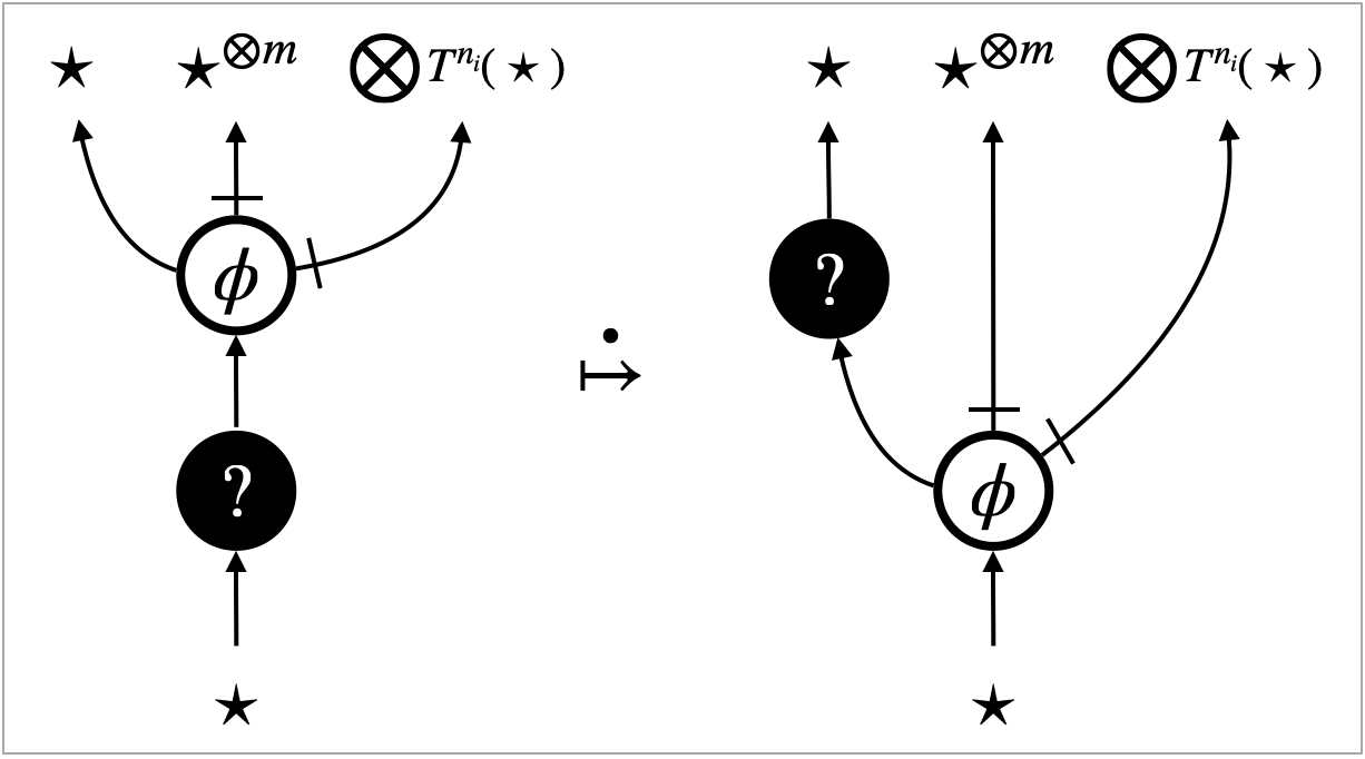
The second case of case analysis for (6) is when the -focus or the -focus encounters one of (and ); see Figure 4b. Let us look at how the micro-beta pre-template (cf. Figure 10b; mind that the focuses are dropped in the pre-template) satisfies (6) in this case. Let be the ones the focus is encountering. There are three sub-cases.
- Case (ii-1) Searching:
-
The -focus enters , i.e. we have and inside states . On , a few search transitions will be followed by a compute transition that applies the micro-beta rewrite rule, because what is connected to the right target of the application edge () (i.e. in Figure 11) is required to be stable. The result is exactly .
This means that we can take a -specimen where: is obtained by replacing the -th hole of with ; and are obtained by removing from . One observation is that the focus in is not entering (i.e. pointing at a hole), because the focus is the -focus pointing at .
- Case (ii-2) Backtracking on the box:
-
The -focus is on top of the box (i.e. in Figure 11). This case is in fact impossible in a refocusing UAM. To make states rooted, the -focus must be at the end of an operation path. However, the -focus in the state is adjacent to a box edge, and cannot be at the end of an operation path.
- Case (ii-3) Backtracking on the stable argument:
-
The -focus is on top of what is connected to the right target of the application edge () (i.e. in Figure 11). This case is also impossible, because of types. The stable hypernet has type (cf. Section 6.1), and the -focus has type . The -focus cannot be on top of .
From Case (ii-1), we extract a sufficient condition for (6), dubbed input-safety, as follows. The micro-beta pre-template falls into (II) below.
{defi}[Input-safety]
A pre-template is
-input-safe if, for any
-specimen
of such that
has the entering -focus, one of the
following holds.
(I)
There exist two stuck states and
such that
for each .
(II)
There exist a -specimen
of
and two numbers , such that
the focus of
is the -focus or the non-entering -focus, ,
, and
.
(III)
There exist a quasi--specimen
of
up to ,
whose focus is not the -focus,
and two numbers ,
such that ,
, and
.
Case (ii-2) and (ii-3) tells us that types and the rooted property prevents the -focus from visiting such that . This situation can be captured by one-way hypernets (Section 6.1), resulting in another sufficient condition dubbed output-closure. {defi}[Output-closure] A pre-template is output-closed if, for any hypernets , either or is one-way.
Input-safety and output-closure are the precise safety conditions. When a pre-template is safe, we simply call it template. {defi}[Templates] A pre-template is a -template, if it is -input-safe and also output-closed.
The micro-beta pre-template is indeed safe, and hence a template. The third parameter of input-safety is irrelevant here, and we can simply set it as the equality . Recall that is the set of all focus-free contexts using operations .
Lemma 4 (Safety of ).
Let be the set , be the set , and . The micro-beta pre-template is a -template. ∎
8.3. Robustness
The last case of case analysis for (6) is when the -focus triggers a rewrite transition in (and hence in ). Does the micro-beta template satisfy (6) in this case? It depends on the rewrite transition . Let us consider an operation set where and . We can perform case analysis in terms of which rewrite is triggered by the -focus.
- Case (iii-1) Substitution:
-
The -focus triggers application of the substitution rule (Figure 9f). The rule simply removes a variable edge (), and the same rule can be applied to both states . Sub-graphs related by may be involved, as part of in Figure 9f, but they are kept unchanged. Therefore we can take a -specimen where has the same number of holes as .
- Case (iii-2) Arithmetic:
-
The -focus triggers application of the arithmetic rewrite rule (Figure 10a). The rewrite rule only involves three edges, and it can never involves sub-graphs related by . We can also take a -specimen where has the same number of holes as .
- Case (iii-3) Micro-beta:
-
The -focus triggers application of the micro-beta rewrite rule (Figure 10b). Sub-graphs related by may be involved in the rewrite rule, as part of the box content in Figure 10b, but they are kept unchanged. We can also take a -specimen where has the same number of holes as .
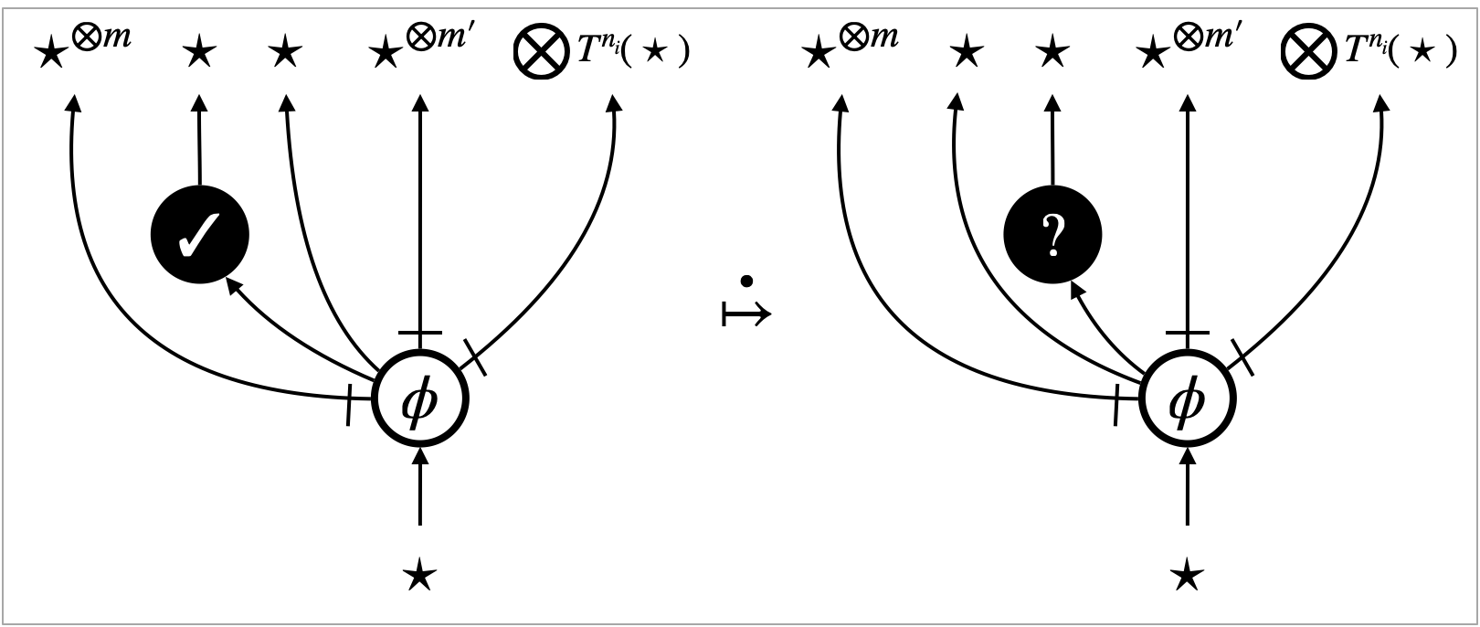
- Case (iii-4) :
-
The -focus triggers application of the rewrite rule (Figure 10c). The rewrite rule inevitably involves sub-graphs related by , and as a result, can yield different results, i.e. vs. . The same rewrite rule can be applied to states and yield , respectively, and these states can contain different natural-number edges (i.e. vs. such that ). We cannot take a specimen of to make (6) happen. ∎
We can therefore observe the following: the micro-beta template satisfies (6) relative to active operations (formalised in 5 below), and does not satisfy (6) relative to the active operation . We say the micro-beta template is robust only relative to .
Robustness, as a sufficient condition for (6), can be formalised as follows.
{defi}[Robustness]
A pre-template is
-robust relative to
a rewrite transition if, for
any -specimen
of , such that
and
the focus of
is the -focus and not entering,
one of the following holds.
(I) or
is not rooted.
(II)
There exists a stuck state such that
.
(III)
There exist a quasi--specimen
of
up to ,
whose focus is not the -focus,
and two numbers ,
such that ,
, and
.
We can now formally say that the micro-beta pre-template is robust relative to the substitution transitions and the extrinsic transitions for . The third and fourth parameters of robustness are irrelevant here555These parameters will be used in Section 12 (See Table 3)., and we can simply set them as the equality .
Lemma 5 (Robustness of ).
The micro-beta pre-template is -robust relative to the substitution transitions and the extrinsic transitions for . ∎
8.4. A sufficiency-of-robustness theorem
We have collected definitions of safety and robustness. We can finally state the sufficiency-of-robustness theorem. The theorem incorporates the so-called up-to technique: it enables us to prove contextual refinement that depends on (or, that is up to) state refinements and . Safety (Section 8.2) and robustness (Section 8.3) accordingly incorporates the up-to technique by means of quasi-specimens up-to. We cannot use arbitrary preorders in combination with the preorder , though; they must be reasonable in the following sense.
[Reasonable triples]
A triple of preorders on is
reasonable if the following hold:
(A) is closed under addition, i.e. any and satisfy
.
(B) , and .
(C) , where denotes
composition of binary relations.
Examples of a reasonable triple include:
,
,
,
,
,
,
,
,
.
The sufficiency-of-robustness theorem has two clauses (1) and (2). To prove that a pre-template implies contextual equivalence (not refinement), one can use (1) twice with respect to and , or alternatively use (1) and (2) with respect to . The alternative approach is often more economical. This is because it involves proving input-safety of for both parameters and , which typically boils down to a single proof for the smaller one of , thanks to monotonicity of input-safety with respect to .
Theorem 6 (Sufficiency-of-robustness theorem).
If an universal abstract machine is deterministic and refocusing, it satisfies the following property. For any set of contexts that is closed under plugging, any reasonable triple , and any pre-template on focus-free hypernets :
-
(1)
If is a -template and -robust relative to all rewrite transitions, then implies contextual refinement in up to , i.e. any implies .
-
(2)
If is a -template and the converse is -robust relative to all rewrite transitions, then implies contextual refinement in up to , i.e. any implies .
Proof 8.1.
This is a consequence of 40, 37 and 38 in Appendix F.
The proof is centred around a notion of counting simulation (Appendix F). We first prove that, for each robust template , its contextual closure is a counting simulation (40). We then prove soundness of counting simulation with respect to state refinement (37). We can further prove that, if implies state refinement, implies contextual refinement (38).
We can use 6 (1) to conclude that the micro-beta pre-template implies contextual refinement . Note that The micro-beta pre-template is -robust, and therefore -robust as well, because .
Proposition 7.
For the operation set , the micro-beta pre-template implies contextual refinement . ∎
The above proposition establishes contextual refinement in the absence of the operation . This is due to the observation that the micro-beta template is not robust relative to the rewrite rule of (Figure 10c). Can we say more than just failure of robustness, in the presence of ?
The answer is yes. For the specific operation set , we can actually show that the micro-beta template implies contextual refinement .
Lemma 8 (Robustness of ).
The micro-beta pre-template is -robust relative to the rewrite transitions for .
Proof 8.2.
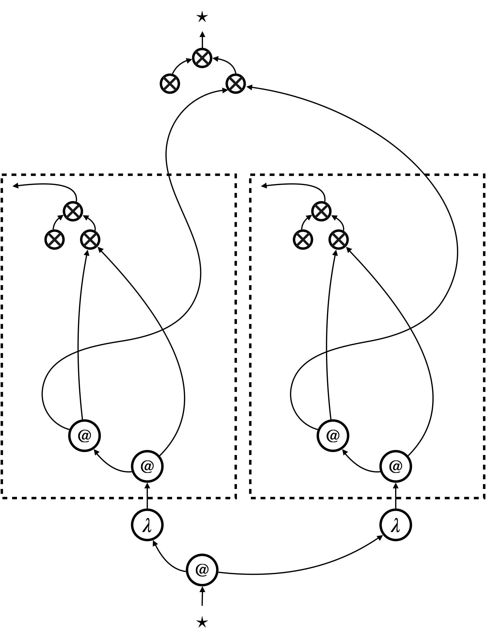
To prove robustness, we use the auxiliary pre-template , shown in Figure 12, that identifies all natural number edges. The pre-template is a -template, and it is -robust relative to the substitution transitions and the extrinsic transitions for including . Therefore, by 6 (1), it implies contextual refinement . The pre-template is symmetric, and consequently, it implies contextual equivalence .
In Case (iii-4) in Section 8.3, we could not take a specimen of that induces the states . The difference between these states is given by as well as different natural number edges; in other words, the difference is given by and .
In fact, we can take a quasi-specimen of up to , which is namely the pair . There exists a state such that: (a) thanks to the symmetric robust template , and (b) the pair is induced by a specimen of .
As a result, with the help of the symmetric robust template , the micro-beta template is robust also relative to .
In the presence of conditional branching and divergence, however, the micro-beta template would not be robust relative to . The above lemma crucially relies on robustness of the auxiliary template , which would be violated by conditional branching; in other words, the template would not be robust relative to conditional branching. Conditional branching and divergence, combined with , would enable us to construct a specific context that distinguishes the left- and the right hand sides of .
9. Representation of variable sharing and store
| Constants: | (natural numbers) | |||
| (booleans) | ||||
| (unit value) | ||||
| Unary operations: | (negation of natural numbers) | |||
| (reference creation) | ||||
| (dereferencing) | ||||
| Binary operations: | (summation/subtraction of natural numbers) | |||
| (assignment) | ||||
| (equality testing of atoms) | ||||
| Terms: | (the lambda-calculus terms) | |||
| (atoms) | ||||
| (constants, unary/binary operations) | ||||
| Formation rules: | ||||
| Syntactic sugar: | ||||
This section adapts the translation of the linear lambda-calculus, presented in Section 4, to accommodate variable sharing and (general, untyped) store. Figure 13 shows an extension of the untyped call-by-value lambda-calculus that accommodates arithmetic as well as:
-
•
atoms (or, locations of store) ,
-
•
reference-related operations: reference creation , dereferencing , assignment , equality testing of atoms ,
-
•
and their return values: booleans and the unit value .
In Figure 13, is a finite sequence of (free) variables and is a finite sequence of (free) atoms.
9.1. Variable sharing
In an arbitrary term, a variable may occur many times, or it may not occur at all. To let sub-terms share and discard a variable, we introduce contraction edges and weakening edges . We can construct a binary tree with an arbitrary number of leaves using these contraction and weakening edges. We call such a tree contraction tree.
There are many ways to construct a contraction tree of leaves, but we fix a canonical666Each is canonical, in the sense that any contraction tree that contains at least one weakening and has leaves can be simplified to using the laws in Figure 21 (namely ). tree as below.
Every canonical tree contains exactly one weakening edge and contraction edges.
The translation of linear lambda-terms needs to be adapted to yield a translation of general lambda-terms. The adaptation amounts to inserting canonical trees appropriately. Additionally, we replace the edges with canonical trees , to obtain uniform translation.
We will present the exact translation in Section 9.3 (see Figure 16), and here we just show an example in Figure 14. Figure 14a shows the hypernet . Canonical trees are inserted for each term constructor, but among those, coloured canonical trees replace the edges that would represent variable occurrences in the linear translation . Figure 14b shows a possible simplification of the hypernet; such simplification is validated only by proving certain observational equivalences on contraction trees (namely, those in Figure 21).
9.2. Store and atom sharing
We next look at terms that contain references to store. An example term is that increments the value stored at atom (location) . We represent such a term, together with store (e.g. ), altogether as a single hypernet; see Figure 15. The hypernets in the figure are simplified in the same manner as Figure 14b.
To represent store and atom sharing, we begin with an observation about the difference between variable sharing and atom sharing. Atoms, like variables, may occur arbitrarily many times in a single term. However, whereas terms bound to a variable can be duplicated, each store associated to the atom should not be duplicated. For example, the atom appears twice in the term , but this does not mean the store is accordingly duplicated. Both occurrences of the atom points at the single store .
This observation leads us to introduce one new vertex label, and some edge labels, of our hypernets. Firstly, we introduce a new vertex label that represents store, in addition to the labels we have used (i.e. for terms and for thunks with bound variables). While terms and thunks can both be duplicated, store cannot be duplicated; this is the reason why we need a new vertex label.
Secondly, we introduce another version of contraction and weakening, namely and , for the type . We call these contraction and weakening as well. Contractions and weakenings for and appear the same, but they will have different behaviours (see Section 10.1).
Finally, we introduce edge labels for type conversion between and : namely, anonymous atom edges called instance , and anonymous store edges . Their roles in the hypernet representation are best understood looking at the example in Figure 15. Each occurrence of an atom is represented by the anonymous instance edge ‘’, and instances of the same atom is connected to a contraction tree of type . The contraction tree is then connected to the part of the hypernet in Figure 15b that represents the store , which consists of the store edge ‘’ and the stored value . In Figure 15b, the part of the hypernet that is typed by connects instances of an atom to its stored value.
To represent sharing of (instances of) atoms, we will use canonical contraction trees that are constructed in the same manner as the canonical trees . Every canonical tree again contains exactly one weakening edge and contraction edges.
9.3. Inductive translation
where are the lengths of respectively.
We now present the translation of the extended lambda-terms into hypernets where
| (7) | ||||
| (8) |
In general, a judgement is translated into where the lengths of are respectively.
The translation uses a generalisation of canonical trees (where ), namely a forest of canonical trees dubbed distributor. A distributor is a forest of canonical trees with some permutation of inputs. It is inserted in the translation for sharing variables/atoms (depending on ) among sub-terms. For instance,
The precise definition of distributors will be given in Section 10.2.
10. The copying UAM
10.1. New behaviour
We equip the UAM with copying, which is the behaviour of contraction edges . The copying UAM acts on hypernets where
| (9) | ||||
For box edges, we impose the following type discipline: each box edge must have a type with its content having a type .
| transitions | focus | provenance | |
|---|---|---|---|
| search transitions | intrinsic | ||
| rewrite transitions | copy transitions | ||
| behaviour | extrinsic | ||
| (compute transitions) | |||
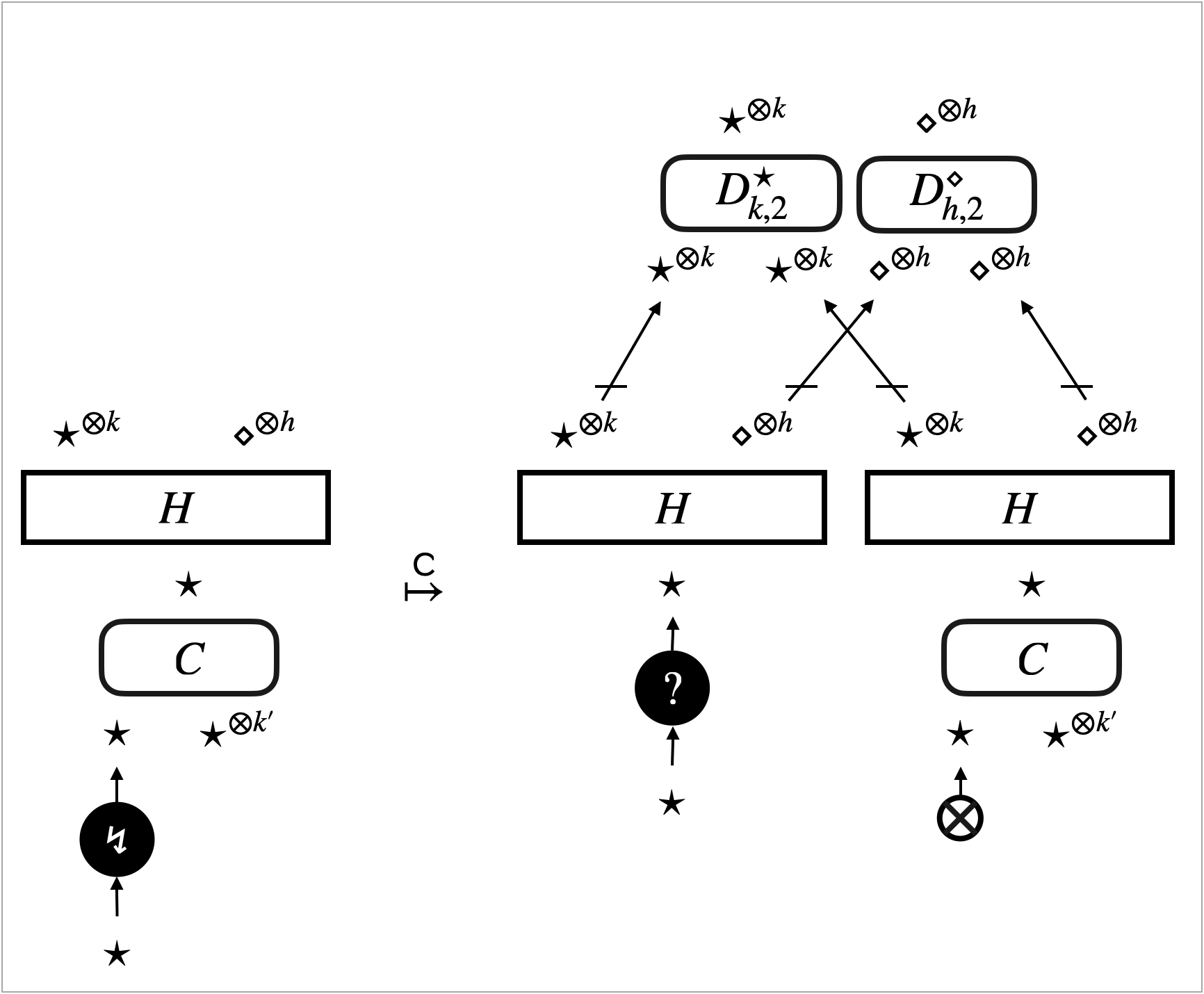
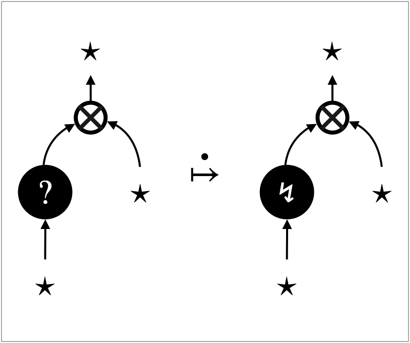

Table 2 summarises transitions of the copying UAM. The copying UAM has copy transitions instead of substitution transitions (cf. Table 1). Copy transitions are specified by the copy rule shown in Figure 17. The copy rule duplicates a copyable hypernet, and inserts distributors and a weakening edge. A copyable hypernet consists of instance edges, operation edges, and box edges. The precise definition of copyable hypernets will be given in Section 10.2. Note that the copy rule only applies to contraction of type ; contraction of type , which are for atoms, do not have a corresponding copy rule. This reflects the fact that atoms are never duplicated unless it is inside a thunk.
Accordingly, the copying UAM has extra search transitions concerning contractions (‘’) and instances (‘’). These are specified by the interaction rules shown in Figure 18.
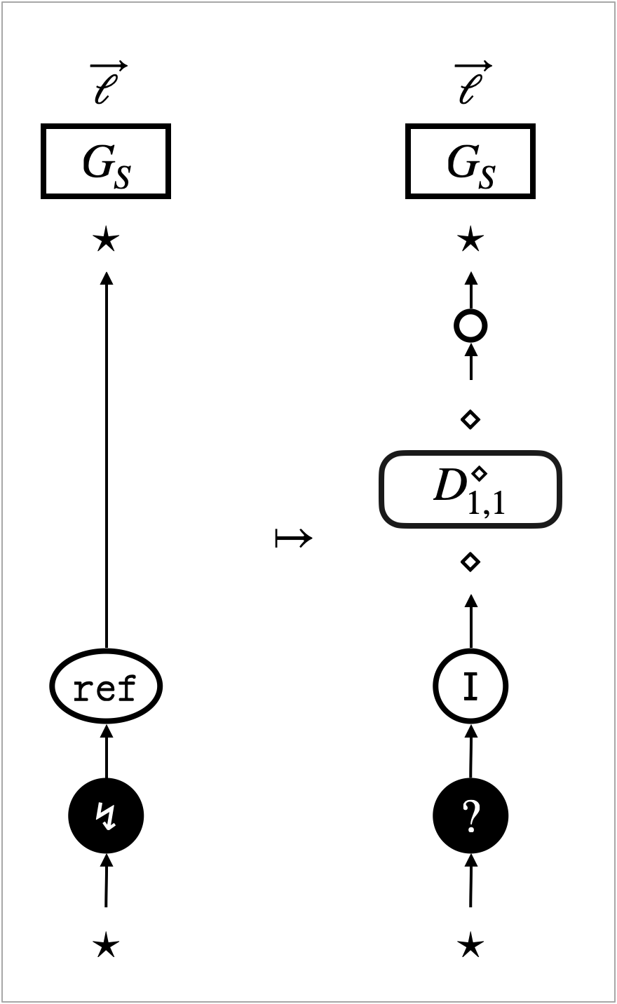
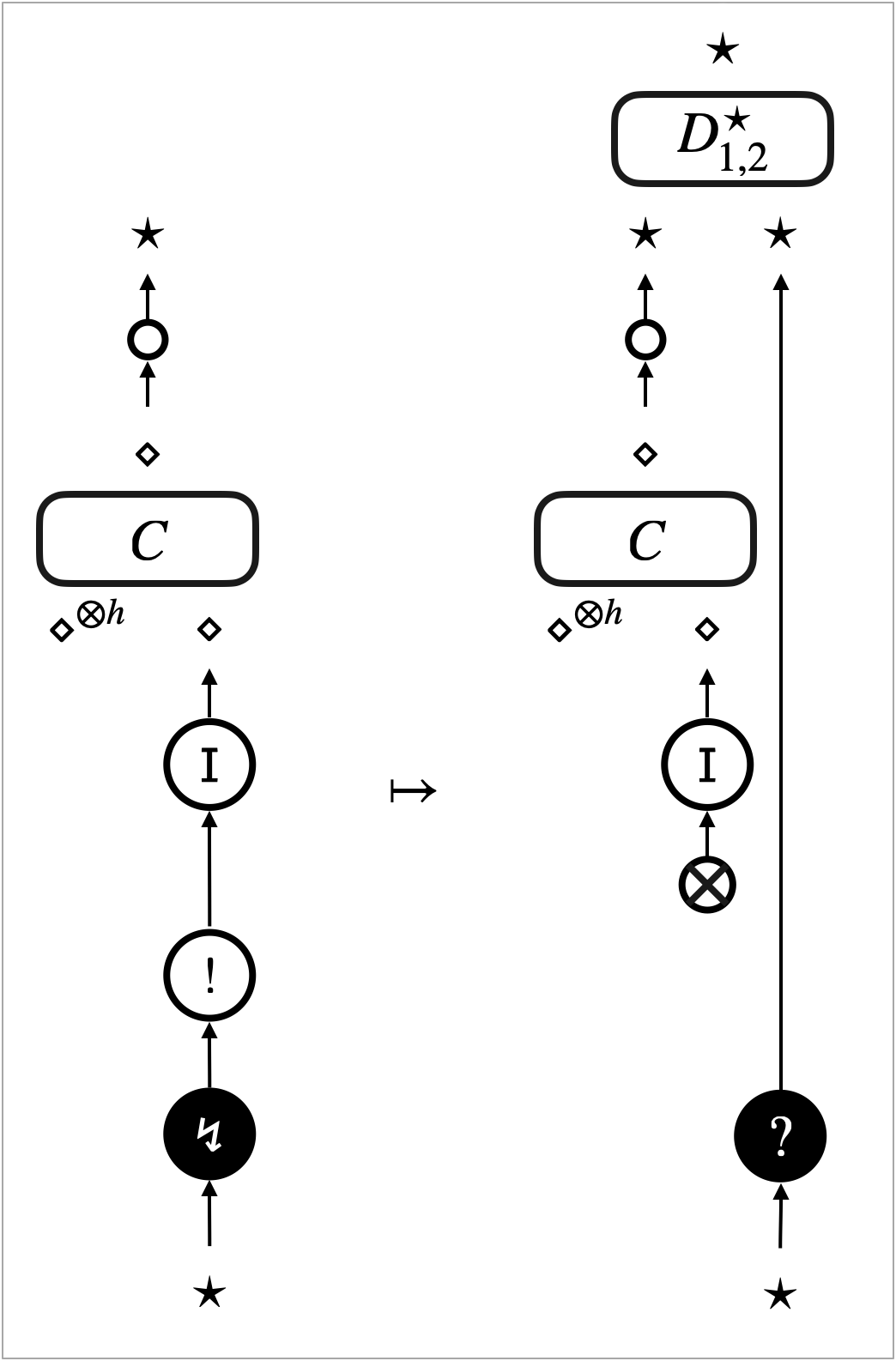
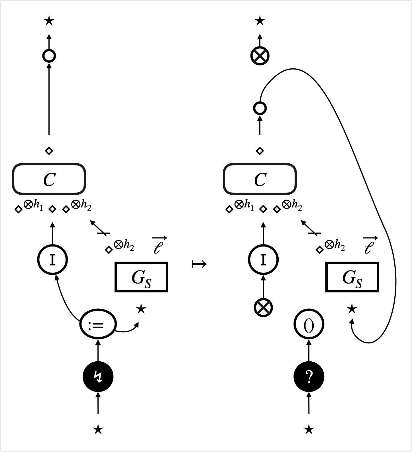
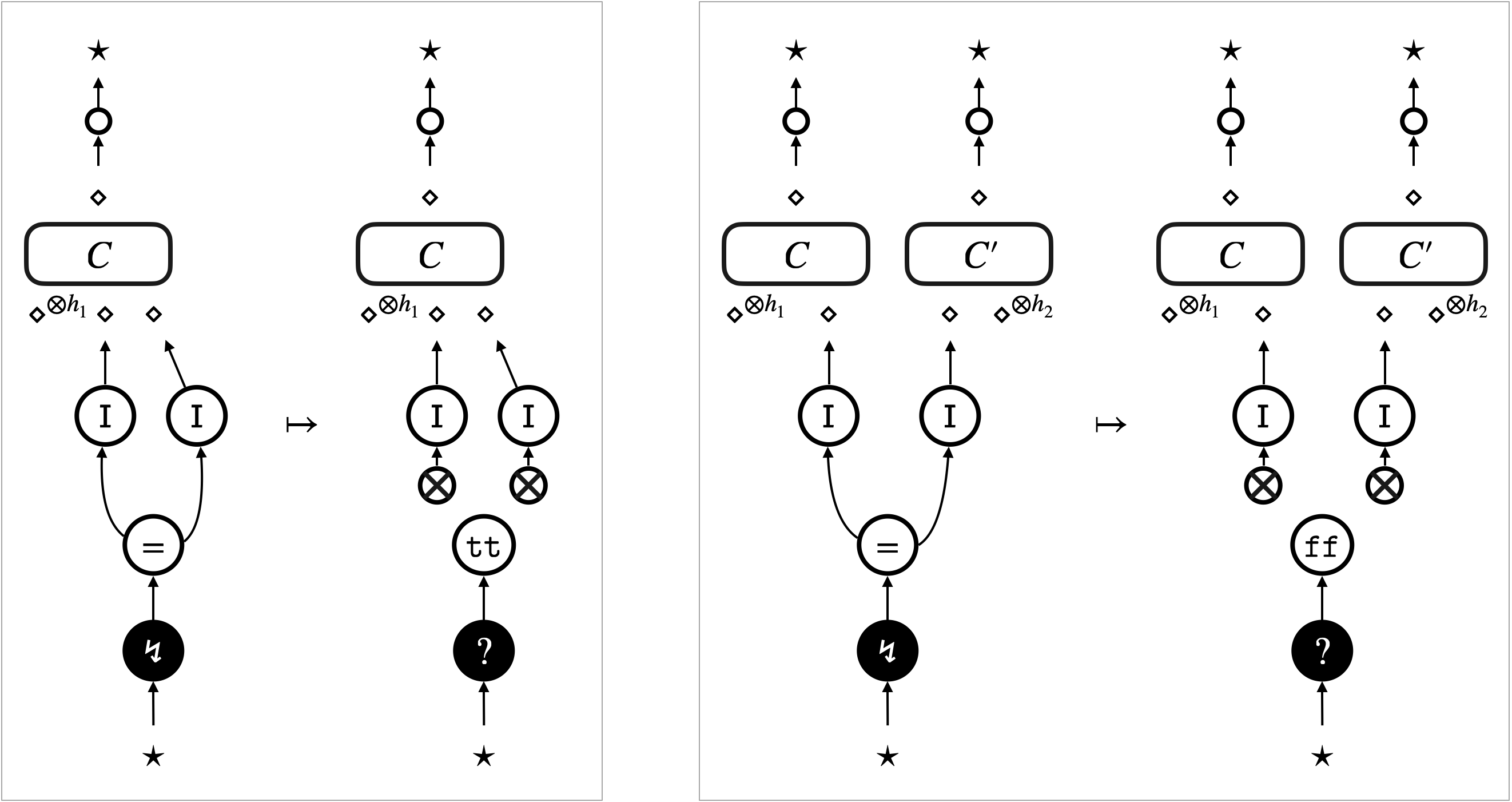
Figure 19 shows an example of the behaviour , namely that for the following active operations for store:
Their behaviour is specified locally by rewrite rules.
- Figure 19a:
-
This rewrite rule specifies the behaviour of reference creation. The rule introduces store (‘’) and its instance (‘’). In between these two edges, a canonical tree is inserted so that there is always a contraction tree between any store and instances.
- Figure 19b:
-
This rewrite rule specifies the behaviour of dereferencing. When dereferencing is triggered, the store edge (‘’) gets attached to a canonical tree , so that its stored value will be copied by subsequent transitions.
- Figure 19c:
-
This rewrite rule specifies the behaviour of assignment. It identifies the store edge (‘’) by tracing the contraction tree connected to the instance edge (‘’). Once the store edge is identified, the current stored value gets disconnected and the new value gets connected to the store edge. Note that the value may contain other instances referring to the same store; this means the rewrite rule may introduce a cycle (via ).
- Figure 19d:
-
This rewrite rule specifies the behaviour of equality testing for atoms. It determines whether two instance edges (‘’) are connected to the same store edge (‘’) or not, by tracing contraction trees . If they are connected to the same store, the result is introduced and attached to the -focus. If not, the result is introduced instead.
10.2. Auxiliary definitions
We here present a few definitions of the concepts introduced so far. The first is distributors. A distributor () is given by a forest of canonical trees whose inputs are permuted. The permutation is realised by interface permutation (Section 3.1). {defi}[Distributors and canonical trees] For and , a distributor is defined inductively as follows.
where denotes the empty hypernet, is the identity map, and is a bijection such that, for each and , and .
When , the distributor is called canonical tree.
The second is copyable hypernets. The copy rule (Figure 17) duplicates a single copyable hypernet at a time. {defi}[Copyable hypernets] A hypernet is called copyable if it is given by
![[Uncaptioned image]](https://cdn.awesomepapers.org/papers/27fdf10b-33e6-4ca5-806a-457df11ca998/copyable-HN-opr.png)
|
where and is a (possibly empty) parallel juxtaposition of box hypernets.
Finally, the notion of stable hypernet (Section 6.1), which corresponds to values, needs to change to incorporate store. {defi}[Stable hypernets] A stable hypernet is a hypernet , such that and each vertex is reachable from the unique input.
10.3. Determinism and refocusing
The properties of determinism and refocusing can be defined for the copying UAM in the same way as the original UAM (cf. Section 7.2). We can again use the stationary property as a sufficient condition for refocusing (2). Determinism and refocusing of a copying UAM also boil down to those of extrinsic transitions under a mild condition.
Lemma 9 (Determinism and refocusing).
-
•
A copying universal abstract machine is deterministic if extrinsic transitions are deterministic.
-
•
Suppose that in the substitution rule (Figure 9f) is a stable hypernet. A copying universal abstract machine is refocusing if extrinsic transitions preserve the rooted property.
Proof 10.1.
The proof is that of 3 equipped with analysis of copying transitions. Copy transitions are all deterministic, because different contraction rules applied to a single state result in the same state. The choice of the contraction tree ( in Figure 17) is irrelevant. Copy transitions are stationary, and hence they preserve the rooted property.
11. Observational equivalence on lambda-terms
Let be the set of operations given by and . The copying UAM provides operational semantics of the extended lambda-calculus (Figure 13). Using contextual equivalence on hypernets (Section 7.1), we can define a notion of observational equivalence on lambda-terms. The notion only concerns the coincidence of termination, which is standard given that the extended lambda-calculus is untyped. {defi}[Observational equivalence on lambda-terms] Let and be two derivable judgements. The lambda-terms and are said to be observationally equivalent, written as , if holds.
This definition uses the specific contextual equivalence . Firstly, the use of the universal relation makes the number of transitions until termination irrelevant. Secondly, the set is the set of all binding-free contexts. {defi}[Binding-free contexts] A focus-free context is said to be binding-free if there exists no path, at any depth, from a source of a contraction, atom, box or hole edge, to a source of a hole edge. For example,
![[Uncaptioned image]](https://cdn.awesomepapers.org/papers/27fdf10b-33e6-4ca5-806a-457df11ca998/ctxt-bf.png) |
is a binding-free context where is a hole. Syntactically it would coincide with a context .
Note that the contextual equivalence is a larger relation than the contextual equivalence with respect to the set of all contexts.
The restriction to binding-free contexts can be justified by the fact that the observational equivalence is a congruence relation with respect to lambda-contexts defined by the following grammar:
where and . This congruence property will be formalised as 10 below.
We can extend the translation to accommodate lambda-contexts. To do so, we first adapt the formation rules of lambda-terms in Figure 13 to lambda-contexts, by annotating the hole ‘’ as ‘’ and adding a formation rule . We write when the hole of is annotated with . The translation of lambda-terms into hypernets in Figure 14 can then be extended accordingly, by translating the additional formation rule into a path hypernet , where and are the length of and respectively.
The translation of lambda-contexts yields hypernets that are binding-free contexts, and consequently, the observational equivalence on lambda-terms is indeed a congruence relation with respect to lambda-contexts.
Lemma 10.
Let and be two derivable judgements. If holds, then for any lambda-context such that is derivable, holds.
Proof 11.1 (Proof outline).
The proof is a combination of the congruence property of the contextual equivalence with respect to binding-free contexts, with two key properties of the translation of lambda-contexts. The two properties, stated below, can be proved by induction on lambda-contexts.
The first property is that the translation is a binding-free context (as a hypernet). To check this property, one needs to examine paths to the sole source of the unique hole edge that appears in the translation. These paths are in fact always operation paths, noting that paths never go across the boundary of boxes (by Section 6.1 (1)).
The second property is that and are both derivable, and moreover, their translations can be decomposed as follows:
12. Example equivalences
In this section we use the sufficiency-of-robustness theorem (6) and prove some example equivalences. The first kind of example is Weakening laws.
Proposition 11 (Weakening laws).
-
•
Given a derivable judgement such that ,
-
•
Given a derivable judgement such that ,
where are the lengths of , respectively.
The next example equivalence is an instance of parametricity. This example originates in the Idealised Algol literature [OT97], a call-by-name language with ground-type local variables, although we state the example for the untyped call-by-value lambda-calculus extended primarily with store (Figure 13). Note that the example uses the standard call-by-value variable binding ‘’ and sequential composition ‘;’, which are both defined by syntactic sugar (see Figure 13).
Proposition 12.
For any finite sequence of distinct variables and any finite sequence of distinct variables ,
| (10) |
In the left hand side (lhs) of (10), a store is created by ‘’, and any access to the store simply fetches the stored value, due to ‘’, without modifying it. As a consequence, the fetched value is always expected to be the original stored value ‘’, and hence the whole computation involving the particular state is expected to have the same result as just having the value ‘’ in the first place as in the right hand side (rhs) of (10).
The equivalence (10) is a typical challenging example in the literature [OT97], which has been proved using parametricity. We take a different approach based on step-wise local reasoning. The equivalence is not an example that is meant to show the full power of our approach; it is a simple yet motivating example that requires building of a whole proof infrastructure and a non-trivial proof methodology.
The rest of this section is organised as follows. Section 12.1 shows prerequisites on the copying UAM . Section 12.2 defines necessary pre-templates, and proves that these imply contextual refinements, using the sufficiency-of-robustness theorem (6). Section 12.3 then combines the resultant contextual refinements to prove the example equivalences (11 & 12). Finally, Section 12.4 describes design process of some of the pre-templates.
12.1. Prerequisites
Here we establish that the particular copying UAM is deterministic and refocusing, which enables us to apply the sufficiency-of-robustness theorem (6). {defi}[the behaviour ] The behaviour is defined locally via the following rewrite rules.
-
•
Rewrite rules for function application are in Figure 10b, where is additionally required to be stable.
-
•
Rewrite rules for reference manipulation are in Figure 19, where is additionally required to be stable.
-
•
Rewrite rules for arithmetic are in Figure 10a.
The extra requirement of stable hypernets reflects the call-by-value nature of the extended lambda-calculus.
Lemma 13.
The copying UAM is deterministic and refocusing.
Proof 12.1.
The proof boils down to show determinism, and preservation of the rooted property, of the compute transitions for , thanks to 9.
Compute transitions of operations are deterministic, because at most one rewrite rule can be applied to each state. In particular, the stable hypernet in the figures is uniquely determined (by 29(3)).
Compute transitions of name-accessing operations are deterministic for the same reason as copy transitions (see the proof of 9).
Compute transitions of all the operations are stationary, and hence they preserve the rooted property. The stationary property can be checked using local rewrite rules. Namely, in each rewrite rule of the operations, only one input of has type , and and . Moreover, any output of with type is a target of an atom edge or a box edge (by definition of stable hypernets), which implies is one-way.
Remark 14 (Requirement of stable hypernets in Section 12.1).
Because any initial state is rooted, given that all transitions preserve the rooted property, we can safely assume that any state that arises in an execution is rooted. This means that the additional requirement of stable hypernets in Section 12.1 is in fact guaranteed to be satisfied in any execution (by 24, 33 and 31). ∎
12.2. Pre-templates and robustness
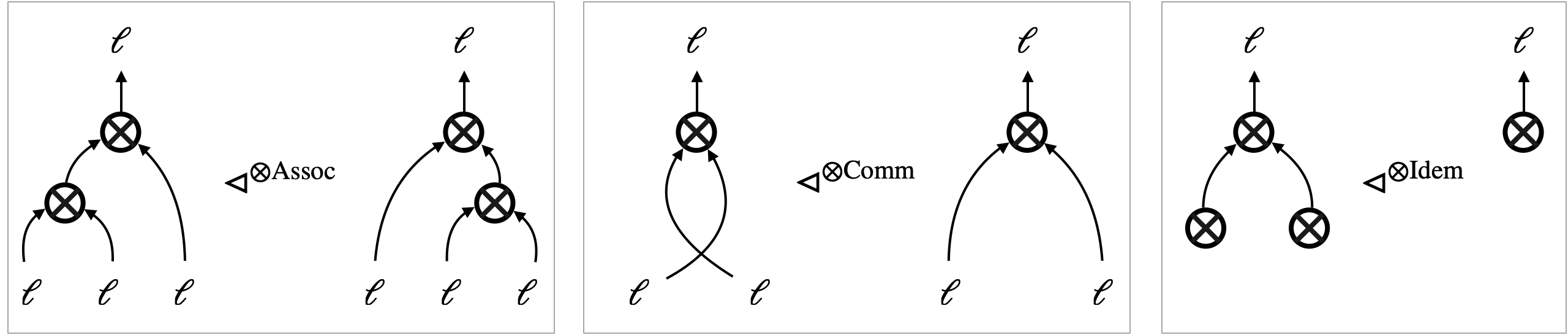
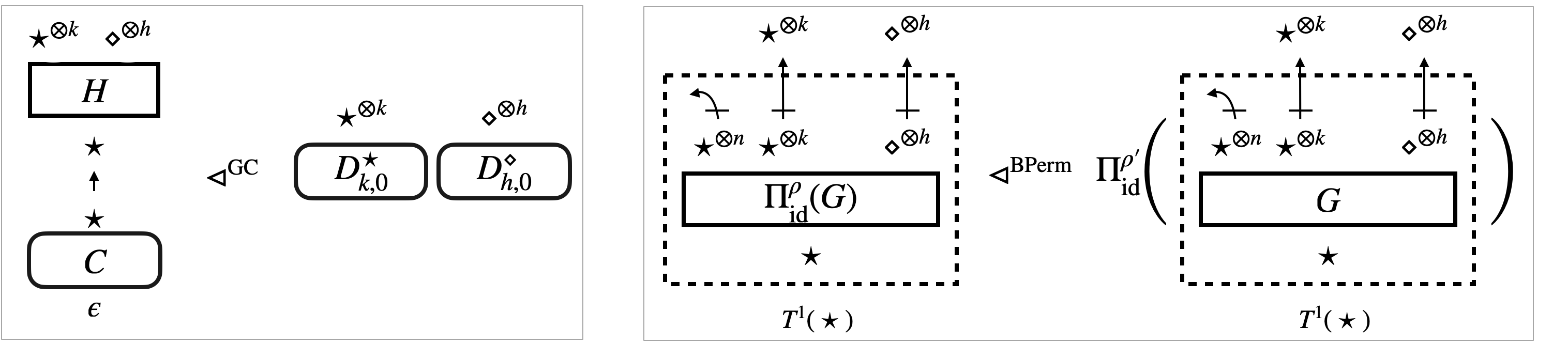
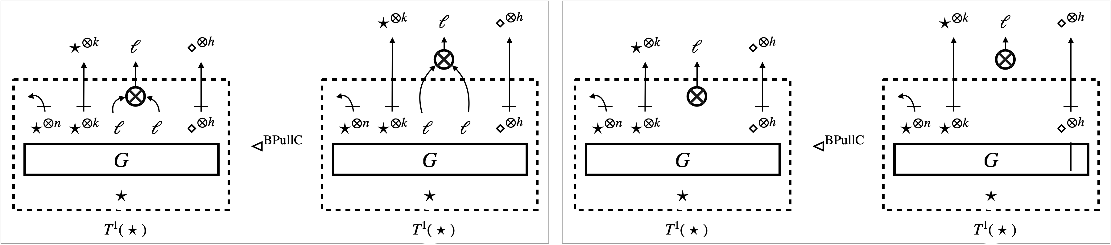
We now define necessary pre-templates, which are the parametricity pre-template , two operational pre-templates and , and structural pre-templates. {defi}[Pre-templates]
-
•
The parametricity pre-template is as shown in Figure 20.
-
•
The micro-beta pre-template is derived from rewrite rules as follows: if is a micro-beta rewrite rule (Figure 10b) where (see the figure) is not an arbitrary hypernet but a stable hypernet.
-
•
The reference-creation pre-template is derived from rewrite rules as follows: if is a reference-creation rewrite rule (Figure 19a) where (see the figure) is not an arbitrary hypernet but a stable hypernet.
-
•
Structural pre-templates are as shown in Figure 21, using the following notion of box-permutation pair.
[Box-permutation pair] For any , let and be bijections on sets and , respectively. These bijections form a box-permutation pair if, for each , the following holds:
-
(1)
if ,
-
(2)
if ,
-
(3)
if ,
-
(4)
if .
The rhs of is straightforward. It simply consists of a bunch of encodings of two function abstractions, namely ‘’ and ‘’. The empty store becomes absent in the graphical representation.
The lhs of contains a bunch of encodings of two function abstractions, i.e. ‘’ and ‘’, and also the graphical representation of the store ‘’ that consists of an atom edge and an edge labelled with the value ‘’. The variable ‘’ refers to the name ‘’, and therefore, the encodings of function abstractions are all connected to the atom edge via a contraction tree.
All structural pre-templates (Figure 21) but concern contractions and weakenings. The pre-template lets us permute outputs of a box.
| template | robustness | ||||
| (input-safety) | of | of | dependency | implication of | |
| — | |||||
| — | |||||
| — | |||||
| — | |||||
| — | |||||
| — | |||||
| — | |||||
Thanks to 13, we can apply the sufficiency-of-robustness theorem (6) and obtain contextual equivalences (on hypernets) as follows.
Lemma 15.
-
(1)
The micro-beta pre-template implies contextual equivalence .
-
(2)
The reference-creation pre-template implies contextual equivalence .
-
(3)
Each structural pre-template implies contextual equivalence .
Proof 12.2 (Proof outline).
Table 3 summarises how we use 6 on the pre-templates. For example, is a -template, as shown in the “template” column, and both itself and its converse are -robust relative to all rewrite transitions, as shown in the “robustness” columns. Thanks to monotonicity of robustness with respect to , we can then use 6(1) with a reasonable triple , and 6(2) with a reasonable triple . Consequently, implies and , which is shown in the “implication of ” column.
Output-closure of the pre-templates can be easily checked, typically by spotting that an input or an output, of type , is a source or a target of a contraction, atom or box edge.
Pre-templates that relate hypernets with no input of type are trivially a -template for any , and . The table uses ‘’ to represent this situation.
Typically, a reasonable triple for a pre-template can be found by selecting “bigger” parameters from those of input-safety and robustness, thanks to monotonicity of input-safety and robustness with respect to . However, the parametricity pre-template requires non-trivial use of the monotonicity. This is because the parameter that makes the pre-template robust, as the upper row in the “robustness” column shows, is not itself a reasonable triple. The lower row shows the alternative, bigger, parameter to which 6 can be applied.
In the table, cyan symbols indicate where a proof of input-safety or robustness relies on contextual refinement. The “dependency” column indicates which pre-templates can be used to prove the necessary contextual refinement, given that these pre-templates imply contextual refinement as shown elsewhere in the table. This reliance specifically happens in finding a quasi-specimen, using contextual refinements/equivalences via 42. In the case of , its input-safety and robustness are proved under the assumption that and imply contextual equivalence .
Detailed proofs of input-safety and robustness are in Section H.2 and Section H.3.
Remark 16 (Necessity of binding-free contexts).
The restriction to binding-free contexts plays a crucial role only in robustness regarding the operational pre-templates and . In fact, these pre-templates are input-safe with respect to both and . This gap reflects duplication behaviour on atom edges, which is only encountered in a proof of robustness.
In fact, robustness of the micro-beta pre-template is not guaranteed in the presence of copy transitions, which apply contraction rules. Starting from a pair of states given by a specimen , it may be the case that some copy transitions are possible without reaching another (quasi-)specimen. An example scenario is when the specimen yields the following two states, where the context is indicated by magenta:
Transitions from the state eventually duplicate the application edge (), the abstraction edge () and also the entire box connected to the abstraction edge. In particular, these transitions duplicate the atom edge contained in the box. However, transitions from the state can never duplicate the atom edge, because the edge is shallow in this state. This mismatch of duplication prevents the micro-beta pre-template from being robust relative to a copy transition.
This is why we restrict contexts to be binding-free, when it comes to robustness of operational pre-templates. If the context is binding-free, the situation explained above would never happen. Application of a contraction rule can involve the hypernets and only as a part of box contents that are duplicated as a whole. Any specimen of is therefore turned into another specimen whose context possibly has more holes, by a single copy transition. Note that this also explains why we allow the context of a specimen to have multiple holes. ∎
12.3. Combining templates
We now combine the contextual equivalences and prove 11 and 12. We start with combining the structural templates and , and prove the Weakening laws.
Proof 12.3 (Proof outline of 11).
The proof is by induction on derivations. Base cases are for variables, atoms and constants. The proof for these cases are trivial, because any distributor with no inputs is simply a bunch of weakening edges (see Section 10.2).
In inductive cases, we need to identify a single weakening edge with a certain (sub-)hypernet, namely: (i) a distributor whose sole input is connected to a weakening edge, (ii) a distributor whose two inputs are connected to weakening edges, and (iii) a distributor whose sole input is connected to a box edge, in which a weakening edge is connected to the corresponding output. The first two situations are for unary/binary operations and function application. These can be handled with the contextual equivalence implied by . The third situation is for function abstraction, and it boils down to the first situation, thanks to the contextual equivalence implied by .
We can then prove the equivalence (10) as follows.
Proof 12.4 (Proof of 12).
Let and be the de-sugared version of the left-hand side and the right-hand side of (10), i.e.:
The equivalence (10) can be obtained as a chain of contextual equivalences whose outline is as follows.
| (11) |
The leftmost and rightmost contextual equivalences are consequences of the Weakening laws (11), because the terms and have no free variables nor free atoms. The middle contextual equivalence follows from the special case of (10) where the environment is empty, i.e. . This contextual equivalence is namely derived from another chain of contextual equivalences that is shown in Figure 22, via the binding-free context that consists of a hole of type and weakening edges (i.e. and ). In Figure 22, each contextual equivalence is accompanied by relevant templates, and preorders on natural numbers are omitted.
This concludes our development leading to the proof our example equivalences.
Table 4 summarises dependency of the example equivalences on templates, which can be observed in the above proofs. The symbol ‘’ indicates direct dependency on templates, in the sense that an equivalence can be proved by combining contextual equivalences implied by these templates. For example, the Weakening laws are obtained by combining two templates and . Because the proof of 12 uses the Weakening law, it also depends on these two templates, which is indicated by ‘(W)’ in the table.
Note that two templates and do not directly appear in the proof of 12, in particular in the chain shown in Figure 22. They are however necessary for robustness of the parametricity template (see Table 3). 12 depends on the two templates only indirectly, which is indicated by the symbol ‘’ in Table 4.
12.4. Designing pre-templates
Chosen terms and contexts:
| (de-sugared version of the lhs of the law) | ||||
| (de-sugared version of the rhs of the law) | ||||
Informal reduction of a program with empty store :
Informal reduction of a program with empty store :
We conclude this section with informal description of how some of the pre-templates are designed, using conventional reduction semantics. This description will reveal how graphical representation is better suited for local reasoning compared to textual representation (see e.g. (12)).
Instead of turning (10) directly into a single pre-template, we decompose the equivalence into several, more primitive, pre-templates. Once we apply the sufficiency-of-robustness theorem to the pre-templates, the obtained contextual equivalences can be composed to yield (10), as we saw in Section 12.3. This approach increases the possibility of reusing parts of a proof of one law in a proof of another law. For example, most of the pre-templates that are used to prove (10) can be reused for proving the call-by-value Beta law (see [Mur20, Section 4.5] for details).
The idea of the pre-templates is that they can describe all the possible differences that may arise during execution of any two programs whose differences is given precisely by (10). As an illustration of the design process, we compare informal reduction sequences of two example programs, as summarised in Figure 23.
We choose the context , which expects a function in the hole and uses it twice. It generates two programs, by receiving the terms and that are a de-sugared version of the two sides of (10).
Each informal reduction step updates a term and its associated store. The step is either the standard call-by-value beta-reduction, addition of numbers (for ‘’), reference creation (for ‘’), or dereferencing (for ‘’). Reference creation is the only step that modifies store. It replaces a (sub-)term of the form ‘’ with a fresh name, say ‘’, and extends the store with ‘’. The empty store is denoted by ‘’. Each reduction step in Figure 23 is given a tag, such as L0, L0’, R1. We use the tags for referring to a corresponding term and store, and also to the reduction step, if any, from the term and store.
Before explaining the colouring scheme of Figure 23, let us observe the (in-)corre-spondence between the reduction sequences of and . The reduction sequence of consists of seven beta-reduction steps (R1–R7) and one addition step (R8). The other reduction sequence, of , in fact contains steps that correspond to these seven beta-reduction steps and the addition step, as suggested by the tags (L1, L2, L3, L4, L5, L6, L7, L8). The sequence has four additional steps, namely: one reference-creation step (L0), one application step (L0’) of a function to the created name ‘’, and two dereferencing steps (L4’, L7’). The two sequences result in the same term, but in different store (L9, R9).
The colouring scheme is as follows. In the eight matching steps and the final result, differences between two sides (e.g. L1 and R1) are highlighted in magenta. Note that it is not the minimum difference that are highlighted. Highlighted parts are chosen in such a way that they capture the smallest difference “on the surface”. Sub-terms on the surface are those that are outside of any lambda-abstraction, which can be graphically represented by sub-hypernets that are outside of any boxes. For example, after the name creation (i.e. in L1, R1), the function abstractions (‘’, ‘’) are highlighted, instead of the minimum difference (‘’, ‘’).
In summary, the reduction sequences of and have eight steps corresponding with each other (L1–L8, R1–R8) where the differences of their results can be described by means of store and sub-terms on the surface. The extracted differences are namely function abstractions (‘’ and ‘’, against ‘’ and ‘’) and store (‘’ against ‘’). By simply collecting these differences, we can obtain our first pre-template: parametricity pre-template . It is the essential, key, pre-template for (10). Textually, and intuitively, it looks like the following.
| (12) |
Graphically, the parametricity pre-template is simply a relation between hypernets (Figure 20). In particular, the lhs of the pre-template can be represented as a single hypernet, thanks to the graphical representation where mentions of a name ‘’ become connection. Hypernets of the function abstractions are all connected to the hypernet of the store ‘’. This graphical representation naturally entails the crucial piece of information, which is invisible in the informal textual representation (12), that the function abstractions are the all and only parts of a program that have access to the name ‘’.
The choice of smallest differences on the surface, instead of absolute minimum difference, also plays a key role here. Should we choose minimum differences that may be inside lambda-abstraction, their hypernet representations cannot be directly combined to yield a single valid hypernet. This is due to the box structure of hypernets, which are used to represent function abstraction. In other words, to connect the hypernet of the store ‘’ to the hypernet of the sub-term ‘’ that appears inside the function abstraction ‘’, we must first make a connection to the hypernet of the whole function abstraction, which contains the hypernet of ‘’ inside a box.
Recall that the parametricity pre-template collects differences in matching steps (eight steps each, i.e. L1–L8, R1–R8). From the first two unmatched steps (L0, L0’), we extract the two operational pre-templates and . These are both induced by the reductions, namely: by reference creation (L0) and by beta-reduction (L0’). For instance, these pre-templates relate the sub-terms that are yielded by the two reductions (L0, L0’), informally as follows.
The three pre-templates , , are all the key pre-templates we needed for (10). Once the sufficiency-of-robustness theorem is applied to these pre-templates, the equivalence can be obtained as a chain of the induced contextual equivalences. The chain roughly looks as follows for the particular programs and , where we use to denote the informal textual counterpart of contextual equivalence that is between terms accompanied by store.
| (13) | |||||
| (induced by ) | |||||
| (induced by ) | |||||
| (induced by ) | |||||
Finally, in the formal proof that uses hypernets and focussed graph rewriting rather than terms and reductions, we additionally needed auxiliary, structural pre-templates (Figure 21). These enable us to simplify or identify certain contractions and weakenings, which are not present in the textual representation but important in the graphical representation as hypernets. Contextual equivalences induced by the structural pre-templates enable simplification of certain hypernets that involve contractions and weakenings. The simplification appeared in the formal counterpart of the chain (13), which is shown in Figure 22. It primarily applies to the hypernets produced by the encoding . Additionally, the pre-templates helped us prove input-safety and robustness of other pre-templates.
13. Related and future work
13.1. Proof methodologies for observational equivalence
This work deals with fragility of observational equivalence and of its proof methodologies. Dreyer et al. address this issue by carefully distinguishing between various kinds of operations (state vs. control) [DNB12]. Dreyer et al. [DNRB10] use Kripke relations to go beyond an enumerative classification of effects; they use characterisation of effects in the aid of reasoning. Their notion of island has similar intuitions to our robustness property. More radical approaches are down to replacing the concept of syntactic context with an epistemic context, akin to a Dolev-Yao-style attacker [GT12], and characterising combinatorially the interaction between a term and its context as is the case with the game semantics [AJM00, HO00] or the trace semantics [JR05]. We propose a new approach to the problem of fragility, namely directly reasoning about robustness of observational equivalence, using a uniform graph representation of a program and its context.
We are not the first one to take a coinductive approach to observational equivalence. Applicative bisimilarity and its successor, environmental bisimilarity, have been successfully used to prove observational equivalence in various effectful settings [Abr90, KLS11, DGL17, SV18]. Typically, one first constructs an applicative (or environmental) bisimulation, and then proves it is a congruence using Howe’s method [How96]. In contrast, in our approach, one first constructs a relation that is closed, by definition, under term (graph) construction, and then proves it is a counting simulation up-to. Our approach does not need Howe’s method.
We argue that our approach is both flexible and elementary. A specific version [MCG18] of this formalism has been used to prove, for example, the soundness of exotic operations involved in (a functional version of) Google’s TensorFlow machine learning library. Even though the proofs can seem complicated, this is in part due to the graph-based formalism being new, and in part due to the fact that proofs of equivalences are lengthy case-based analyses. However, herein lies the simplicity and the robustness of the approach, avoiding the discovery of clever-but-fragile language invariants which can be used to streamline proofs.
Our tedious-but-elementary proofs on the other hand seem highly suitable for automation. The idea of elementary case analysis can be adopted in term rewriting, instead of hypernet rewriting, for a call-by-value lambda-calculus equipped with effect handlers [Pre15]. In this setting, the case analysis can be formalised as critical pair analysis, which is a fundamental and automatable technique in term rewriting, and indeed automated [MH24].
13.2. Focussed hypernet rewriting
Focussed hypernet rewriting is a radically new approach to defining effectful programming languages and proving observational equivalence. We are not so much interested in simulated effects, which are essentially the encoding of effectful behaviour into pure languages, and which can be achieved via monads [Wad98], but we are interested in genuine native effects which happen outside of the language. Semantically this has been introduced by Plotkin and Power [PP08] and more recently developed by Møgelberg and Staton [MS11]. The (copying) UAM takes the idea to the extreme by situating all operations (pure or effectful) outside of the primitives, and by keeping as intrinsic to the language only the structural aspects of copying vs. sharing, and scheduling of computation via thunking.
The (copying) UAM presented in this paper is an extension of the Dynamic Geometry of Interaction Machine (DGoIM) [MG17] to effects. The DGoIM builds on operational machinery [DR96, Mac95, HMH14, MHH16] inspired by Girard’s Geometry of Interaction (GoI) [Gir89]. Unlike these “conventional” GoI-inspired operational semantics, the DGoIM and hence the UAM are modified so that the underlying hypernet can be rewritten during execution.
The original motivation of the DGoIM was to produce an abstract machine that expresses the computational intuitions of the GoI while correctly modelling the cost of evaluation, particularly for call-by-value and call-by-need. The ability to rewrite its own hypernet makes the DGoIM efficient, in the sense of Accattoli et al. [ABM14], for common reduction strategies (namely, call-by-value and call-by-need). It also gives the DGoIM the ability to model exotic effects, e.g. transforming stateful into pure computation by abstracting the state [MCG18]. As an extension of the DGoIM, the UAM is designed for new reasoning principles and methods that arise out of GoI-inspired operational semantics.
Although the UAM does not aim at efficiency at the moment, one can think of a cost model of the UAM in a similar way as the DGoIM. Moreover, the indexing of observational equivalence with a preorder representing the number of steps gives a direct avenue for modelling and comparing computation costs. For example, the micro-beta law induced by the pre-template is indexed by the normal order on (cf. Table 3), which indicates that one side always requires fewer steps than the other in the evaluation process. The only details to be resolved are associating costs (time and space) with steps, in particular different costs for different operations.
The UAM is motivated by a need for a flexible and expressive framework in which a wide variety of effects can be given a cost-accurate model. As discussed, the UAM opens the door to a uniform study of operations and their interactions. Defining new styles of abstract machines is a rich and attractive vein of research. The monoidal computer of Pavlovic [Pav13] or the evolving algebras of Gurevich [Gur18] are such examples. What sets the UAM apart is the fact that it can be used, rather conveniently, for reasoning robustly about observational equivalence.
13.3. Hypernets
The hierarchy of hypernets is inspired by the exponential boxes of proof nets, a graphical representation of linear logic proofs [Gir87] and have an informal connection to Milner’s bigraphs [Mil01]. Exponential boxes can be formalised by parameterising an agent (which corresponds to an edge in our setting) by a net, as indicated by Lafont [Laf95]. In the framework of interaction nets [Laf90] that subsume proof nets, agents can be coordinated to represent a boundary of a box, as suggested by Mackie [Mac98]. An alternative representation of boxes that use extra links between agents is proposed by Accattoli and Guerrini [AG09].
Our graphical formulation of boxes shares the idea with the first parameterising approach, but we have flexibility regarding types of a box edge itself and its content (i.e. the hypernet that labels it). We use box edges to represent thunks, and a box edge can have less targets than outputs of its contents, reflecting the number of bound variables a thunk has. This generalised box structure is also studied by Drewes et al. [DHP02] as hierarchical graphs, in the context of double-pushout graph transformation (DPO) [Roz97], an well-established algebraic approach to graph rewriting. More recently, Alvarez-Picallo et al. have formulated DPO rewriting for a class of hypernets similar to those used here [AGSZ22]; their work further relates hypernets with string diagrams with functorial boxes in the style of Melliès [Mel06].
Interaction nets are another established framework of graph rewriting, in which various evaluations of pure lambda-calculus can be implemented [Sin05, Sin06]. The idea of having the token to represent an evaluation strategy can be found in loc. cit., which suggests that our focussed rewriting on hypernets could be implemented using interaction nets. However, the local reasoning we are aiming at with focussed rewriting does not seem easy in the setting of interaction nets, because of technical subtleties observed in loc. cit.; namely, a status of evaluation is remembered by not only the token but also some other agents around an interaction net.
13.4. Future work
One direction is the introduction of a more meaningful type system for hypernets. The current type system of hypernets is very weak, just ensuring well-formedness. We consider it a strength of the approach that equivalences can be proved without the aid of a powerful type infrastructure. On the other hand, in order to avoid stuck configurations and ensure safety of evaluation, more expressive types are required. The usage of more expressive types is perfectly compatible with focussed hypernet rewriting, and is something we intend to explore. In particular we would like to study notions of typing which are germane to focussed hypernet rewriting, capturing its concepts of locality and robustness.
Beyond types, if we look at logics there are some appealing similarities between hypernet rewriting and separation logic [Rey02]. The division of nodes into copying nodes via variables and sharing nodes via atoms is not accidental, and their different contraction properties match those from bunched implications [OP99]. On a deeper level, the concepts of locality and in particular robustness developed here are related to the frame rule of separation logic.
Finally, our formulation of equivalence has some self-imposed limitations needed to limit the complexity of the technical presentation. We are hereby concerned with sequential and deterministic computation. Future work will show how these restrictions can be relaxed. Parallelism and concurrency can be naturally simulated using multi-token reductions, as inspired by the multi-token GoI machine of Dal Lago et al. [DTY17], whereas nondeterminism (or probabilistic evaluation) requires no changes to the machinery but rather a new definition of observational equivalence. This is work we are aiming to undertake in the future. A first step towards nondeterminism has been made [MSU24] in which the notion of counting simulation is extended from branching-free transition systems to nondeterministic automata.
References
- [ABM14] Beniamino Accattoli, Pablo Barenbaum, and Damiano Mazza. Distilling abstract machines. In 19th ACM SIGPLAN International Conference on Functional Programming, ICFP 2014, September 1-3 2014, Gothenburg, Sweden, pages 363–376, 2014. doi:10.1145/2628136.2628154.
- [Abr90] Samson Abramsky. The lazy lambda-calculus, page 65–117. Addison Wesley, 1990.
- [Abr97] Samson Abramsky. Game semantics for programming languages. In 22nd International Symposium on Mathematical Foundations of Computer Science, MFCS 1997, August 25-29 1997, Bratislava, Slovakia, pages 3–4, 1997. doi:10.1007/BFb0029944.
- [ADV20] Beniamino Accattoli, Ugo Dal Lago, and Gabriele Vanoni. The machinery of interaction. In PPDP 2020, pages 4:1–4:15. ACM, 2020.
- [ADV21] Beniamino Accattoli, Ugo Dal Lago, and Gabriele Vanoni. The (in)efficiency of interaction. Proc. ACM Program. Lang., 5(POPL):1–33, 2021. doi:10.1145/3434332.
- [AG09] Beniamino Accattoli and Stefano Guerrini. Jumping boxes. In CSL 2009, volume 5771 of Lect. Notes Comp. Sci., pages 55–70. Springer, 2009. doi:10.1007/978-3-642-04027-6_7.
- [AGSZ22] Mario Alvarez-Picallo, Dan R. Ghica, David Sprunger, and Fabio Zanasi. Rewriting for monoidal closed categories. In Amy P. Felty, editor, 7th International Conference on Formal Structures for Computation and Deduction, FSCD 2022, August 2-5, 2022, Haifa, Israel, volume 228 of LIPIcs, pages 29:1–29:20. Schloss Dagstuhl - Leibniz-Zentrum für Informatik, 2022. doi:10.4230/LIPICS.FSCD.2022.29.
- [AGSZ23] Mario Alvarez-Picallo, Dan R. Ghica, David Sprunger, and Fabio Zanasi. Functorial string diagrams for reverse-mode automatic differentiation. In Bartek Klin and Elaine Pimentel, editors, 31st EACSL Annual Conference on Computer Science Logic, CSL 2023, February 13-16, 2023, Warsaw, Poland, volume 252 of LIPIcs, pages 6:1–6:20. Schloss Dagstuhl - Leibniz-Zentrum für Informatik, 2023. doi:10.4230/LIPICS.CSL.2023.6.
- [AJM00] Samson Abramsky, Radha Jagadeesan, and Pasquale Malacaria. Full abstraction for PCF. Inf. Comput., 163(2):409–470, 2000. doi:10.1006/INCO.2000.2930.
- [BGK+22a] Filippo Bonchi, Fabio Gadducci, Aleks Kissinger, Pawel Sobocinski, and Fabio Zanasi. String diagram rewrite theory I: rewriting with frobenius structure. J. ACM, 69(2):14:1–14:58, 2022. doi:10.1145/3502719.
- [BGK+22b] Filippo Bonchi, Fabio Gadducci, Aleks Kissinger, Pawel Sobocinski, and Fabio Zanasi. String diagram rewrite theory II: rewriting with symmetric monoidal structure. Math. Struct. Comput. Sci., 32(4):511–541, 2022. doi:10.1017/S0960129522000317.
- [BGK+22c] Filippo Bonchi, Fabio Gadducci, Aleks Kissinger, Pawel Sobocinski, and Fabio Zanasi. String diagram rewrite theory III: confluence with and without frobenius. Math. Struct. Comput. Sci., 32(7):829–869, 2022. doi:10.1017/S0960129522000123.
- [BPPR17] Filippo Bonchi, Daniela Petrisan, Damien Pous, and Jurriaan Rot. A general account of coinduction up-to. Acta Inf., 54(2):127–190, 2017. doi:10.1007/s00236-016-0271-4.
- [DGL17] Ugo Dal Lago, Francesco Gavazzo, and Paul Blain Levy. Effectful applicative bisimilarity: Monads, relators, and howe’s method. In 32nd Annual ACM/IEEE Symposium on Logic in Computer Science, LICS 2017, Reykjavik, Iceland, June 20-23, 2017, pages 1–12. IEEE Computer Society, 2017. doi:10.1109/LICS.2017.8005117.
- [DHP02] Frank Drewes, Berthold Hoffmann, and Detlef Plump. Hierarchical graph transformation. J. Comput. Syst. Sci., 64(2):249–283, 2002. doi:10.1006/jcss.2001.1790.
- [DMMZ12] Olivier Danvy, Kevin Millikin, Johan Munk, and Ian Zerny. On inter-deriving small-step and big-step semantics: A case study for storeless call-by-need evaluation. Theor. Comput. Sci., 435:21–42, 2012. doi:10.1016/j.tcs.2012.02.023.
- [DNB12] Derek Dreyer, Georg Neis, and Lars Birkedal. The impact of higher-order state and control effects on local relational reasoning. J. Funct. Program., 22(4-5):477–528, 2012. doi:10.1017/S095679681200024X.
- [DNRB10] Derek Dreyer, Georg Neis, Andreas Rossberg, and Lars Birkedal. A relational modal logic for higher-order stateful adts. In Proceedings of the 37th Annual ACM SIGPLAN-SIGACT Symposium on Principles of Programming Languages, POPL ’10, pages 185–198, New York, NY, USA, 2010. ACM. doi:10.1145/1706299.1706323.
- [DR96] Vincent Danos and Laurent Regnier. Reversible, irreversible and optimal lambda-machines. Elect. Notes in Theor. Comp. Sci., 3:40–60, 1996.
- [DTY17] Ugo Dal Lago, Ryo Tanaka, and Akira Yoshimizu. The geometry of concurrent interaction: Handling multiple ports by way of multiple tokens. In 32nd Annual ACM/IEEE Symposium on Logic in Computer Science, LICS 2017, Reykjavik, Iceland, June 20-23, 2017, pages 1–12, 2017. doi:10.1109/LICS.2017.8005112.
- [Ghi23] Dan R. Ghica. The far side of the cube. In Alessandra Palmigiano and Mehrnoosh Sadrzadeh, editors, Samson Abramsky on Logic and Structure in Computer Science and Beyond, pages 219–250. Springer Verlag, 2023.
- [Gir87] Jean-Yves Girard. Linear logic. Theor. Comput. Sci., 50:1–102, 1987. doi:10.1016/0304-3975(87)90045-4.
- [Gir89] Jean-Yves Girard. Geometry of Interaction I: interpretation of system F. In Logic Colloquium 1988, volume 127 of Studies in Logic & Found. Math., pages 221–260. Elsevier, 1989.
- [GT12] Dan R. Ghica and Nikos Tzevelekos. A system-level game semantics. Electr. Notes Theor. Comput. Sci., 286:191–211, 2012. doi:10.1016/j.entcs.2012.08.013.
- [Gur18] Yuri Gurevich. Evolving algebras 1993: Lipari guide. arXiv preprint arXiv:1808.06255, 2018.
- [GZ23] Dan Ghica and Fabio Zanasi. String diagrams for -calculi and functional computation. arXiv preprint arXiv:2305.18945, 2023.
- [HMH14] Naohiko Hoshino, Koko Muroya, and Ichiro Hasuo. Memoryful geometry of interaction: from coalgebraic components to algebraic effects. In Joint Meeting of the 23rd EACSL Annual Conference on Computer Science Logic (CSL) and the 29th Annual ACM/IEEE Symposium on Logic in Computer Science (LICS), CSL-LICS 2014, July 14-18 2014, Vienna, Austria, pages 52:1–52:10, 2014. doi:10.1145/2603088.2603124.
- [HO00] J. M. E. Hyland and C.-H. Luke Ong. On full abstraction for PCF: I, II, and III. Inf. Comput., 163(2):285–408, 2000. doi:10.1006/inco.2000.2917.
- [How96] Douglas J. Howe. Proving congruence of bisimulation in functional programming languages. Inf. Comput., 124(2):103–112, 1996. doi:10.1006/INCO.1996.0008.
- [JR05] Alan Jeffrey and Julian Rathke. Java jr: Fully abstract trace semantics for a core java language. In 14th European Symposium on Programming, ESOP 2005, Held as Part of the Joint European Conferences on Theory and Practice of Software, ETAPS 2005, April 4-8 2005, Edinburgh, UK, pages 423–438, 2005. doi:10.1007/978-3-540-31987-0\_29.
- [KLS11] Vasileios Koutavas, Paul Blain Levy, and Eijiro Sumii. From applicative to environmental bisimulation. In Michael W. Mislove and Joël Ouaknine, editors, Twenty-seventh Conference on the Mathematical Foundations of Programming Semantics, MFPS 2011, Pittsburgh, PA, USA, May 25-28, 2011, volume 276 of Electronic Notes in Theoretical Computer Science, pages 215–235. Elsevier, 2011. doi:10.1016/J.ENTCS.2011.09.023.
- [Laf90] Yves Lafont. Interaction nets. In 17th Annual ACM Symposium on Principles of Programming Languages, POPL 1990, January 1990, San Francisco, California, USA, pages 95–108, 1990. doi:10.1145/96709.96718.
- [Laf95] Yves Lafont. From proof nets to interaction nets, page 225–248. London Mathematical Society Lecture Note Series. Cambridge University Press, 1995. doi:10.1017/CBO9780511629150.012.
- [Mac95] Ian Mackie. The Geometry of Interaction machine. In POPL 1995, pages 198–208. ACM, 1995.
- [Mac98] Ian Mackie. Linear logic With boxes. In 13th IEEE Symposium on Logic in Computer Science, June 21-24 1998, Indianapolis, IN, USA, pages 309–320, 1998. doi:10.1109/LICS.1998.705667.
- [MCG18] Koko Muroya, Steven W. T. Cheung, and Dan R. Ghica. The geometry of computation-graph abstraction. In Proceedings of the 33rd Annual ACM/IEEE Symposium on Logic in Computer Science, LICS 2018, Oxford, UK, July 09-12 2018, pages 749–758, 2018. doi:10.1145/3209108.3209127.
- [Mel06] Paul-André Melliès. Functorial boxes in string diagrams. In 20th International Workshop on Computer Science Logic, CSL 2006, 15th Annual Conference of the EACSL, September 25-29 2006, Szeged, Hungary, pages 1–30, 2006. doi:10.1007/11874683\_1.
- [MG17] Koko Muroya and Dan R. Ghica. The dynamic geometry of interaction machine: A call-by-need graph rewriter. In 26th EACSL Annual Conference on Computer Science Logic, CSL 2017, August 20-24 2017, Stockholm, Sweden, pages 32:1–32:15, 2017. doi:10.4230/LIPIcs.CSL.2017.32.
- [MH24] Koko Muroya and Makoto Hamana. Term evaluation systems with refinements: First-order, second-order, and contextual improvement. In Jeremy Gibbons and Dale Miller, editors, Functional and Logic Programming - 17th International Symposium, FLOPS 2024, Kumamoto, Japan, May 15-17, 2024, Proceedings, volume 14659 of Lecture Notes in Computer Science, pages 31–61. Springer, 2024. doi:10.1007/978-981-97-2300-3\_3.
- [MHH16] Koko Muroya, Naohiko Hoshino, and Ichiro Hasuo. Memoryful geometry of interaction II: recursion and adequacy. In Proceedings of the 43rd Annual ACM SIGPLAN-SIGACT Symposium on Principles of Programming Languages, POPL 2016, St. Petersburg, FL, USA, January 20-22 2016, pages 748–760, 2016. doi:10.1145/2837614.2837672.
- [Mil01] Robin Milner. Bigraphical reactive systems. In International Conference on Concurrency Theory, pages 16–35. Springer, 2001. doi:10.1007/3-540-44685-0_2.
- [MJ69] James Hiram Morris Jr. Lambda-calculus models of programming languages. PhD thesis, Massachusetts Institute of Technology, 1969. URL: https://dspace.mit.edu/handle/1721.1/64850.
- [MS11] Rasmus Ejlers Møgelberg and Sam Staton. Linearly-used state in models of call-by-value. In 4th International Conference on Algebra and Coalgebra in Computer Science, CALCO 2011, August 30 - September 2 2011, Winchester, UK, pages 298–313, 2011. doi:10.1007/978-3-642-22944-2\_21.
- [MSU24] Koko Muroya, Takahiro Sanada, and Natsuki Urabe. Preorder-constrained simulations for program refinement with effects. In CMCS 2024, 2024. To appear.
- [Mur20] Koko Muroya. Hypernet Semantics of Programming Languages. PhD thesis, University of Birmingham, 2020.
- [OP99] Peter W O’Hearn and David J Pym. The logic of bunched implications. Bulletin of Symbolic Logic, 5(2):215–244, 1999. doi:10.2307/421090.
- [OT97] Peter O’Hearn and Robert Tennent, editors. Algol-like languages. Progress in theoretical computer science. Birkhauser, 1997. doi:10.1007/978-1-4612-4118-8.
- [Pav13] Dusko Pavlovic. Monoidal computer I: Basic computability by string diagrams. Information and Computation, 226:94–116, 2013. doi:10.1016/j.ic.2013.03.007.
- [Pit00] Andrew M. Pitts. Operational semantics and program equivalence. In Gilles Barthe, Peter Dybjer, Luís Pinto, and João Saraiva, editors, Applied Semantics, International Summer School, APPSEM 2000, Caminha, Portugal, September 9-15, 2000, Advanced Lectures, volume 2395 of Lecture Notes in Computer Science, pages 378–412. Springer, 2000. doi:10.1007/3-540-45699-6\_8.
- [PP08] Gordon D. Plotkin and John Power. Tensors of comodels and models for operational semantics. Electr. Notes Theor. Comput. Sci., 218:295–311, 2008. doi:10.1016/j.entcs.2008.10.018.
- [Pre15] Matija Pretnar. An introduction to algebraic effects and handlers. invited tutorial paper. Elect. Notes in Theor. Comp. Sci., 319:19–35, 2015.
- [Rey02] John C Reynolds. Separation logic: A logic for shared mutable data structures. In Proceedings 17th Annual IEEE Symposium on Logic in Computer Science, pages 55–74. IEEE, 2002. doi:10.1109/LICS.2002.1029817.
- [Roz97] Grzegorz Rozenberg, editor. Handbook of graph grammars and computing by graph transformations, volume 1: foundations. World Scientific, 1997.
- [San95] David Sands. Total correctness by local improvement in program transformation. In Ron K. Cytron and Peter Lee, editors, Conference Record of POPL’95: 22nd ACM SIGPLAN-SIGACT Symposium on Principles of Programming Languages, San Francisco, California, USA, January 23-25, 1995, pages 221–232. ACM Press, 1995. doi:10.1145/199448.199485.
- [Sin05] François-Régis Sinot. Call-by-name and call-by-value as token-passing interaction nets. In 7th International Conference on Typed Lambda Calculi and Applications, TLCA 2005, April 21-23 2005, Nara, Japan, pages 386–400, 2005. doi:10.1007/11417170\_28.
- [Sin06] François-Régis Sinot. Call-by-need in token-passing nets. Mathematical Structures in Computer Science, 16(4):639–666, 2006. doi:10.1017/S0960129506005408.
- [SKS07] Davide Sangiorgi, Naoki Kobayashi, and Eijiro Sumii. Environmental bisimulations for higher-order languages. In LICS 2007, pages 293–302. IEEE Computer Society, 2007.
- [Sta85] Richard Statman. Logical relations and the typed lambda-calculus. Information and Control, 65(2/3):85–97, 1985. doi:10.1016/S0019-9958(85)80001-2.
- [SV18] Alex Simpson and Niels F. W. Voorneveld. Behavioural equivalence via modalities for algebraic effects. In Amal Ahmed, editor, Programming Languages and Systems - 27th European Symposium on Programming, ESOP 2018, Held as Part of the European Joint Conferences on Theory and Practice of Software, ETAPS 2018, Thessaloniki, Greece, April 14-20, 2018, Proceedings, volume 10801 of Lecture Notes in Computer Science, pages 300–326. Springer, 2018. doi:10.1007/978-3-319-89884-1\_11.
- [Wad98] Philip Wadler. The marriage of effects and monads. In ACM SIGPLAN Notices, volume 34:1, pages 63–74. ACM, 1998. doi:10.1145/289423.289429.
Appendix A An alternative definition of hypernets
Informally, hypernets are nested hypergraphs, and one hypernet can contain nested hypergraphs up to different depths. This intuition is reflected by footnote 3 of hypernets, in particular the big union in . In fact, the definition can be replaced by a simpler, but possibly less intuitive, definition below that does not explicitly deal with the different depths of nesting. {defi} Given sets and , a set is defined by induction on :
and hence a set .
Lemma 17.
Given arbitrary sets and , any two numbers satisfy .
Proof A.1.
If , the inclusion trivially holds. If not, i.e. , it can be proved by induction on . The key reasoning principle we use is that implies .
In the base case, when (and ), we have
In the inductive case, when (and ), we have
where the inclusion is by induction hypothesis on .
Proposition 18.
Any sets and satisfy for any , and hence .
Proof A.2.
We first prove by induction on . The base case, when , is trivial. In the inductive case, when , we have
| (by I.H.) | ||||
| (by 17) | ||||
The other direction, i.e. , can be also proved by induction on . The base case, when , is again trivial. In the inductive case, we have
| (by I.H.) | ||||
Given a hypernet , by 17 and 18, there exists a minimum number such that , which we call the “minimum level” of .
Lemma 19.
Any hypernet has a finite number of shallow edges, and a finite number of deep edges.
Proof A.3.
Any hypernet has a finite number of shallow edges by definition. We prove that any hypernet has a finite number of deep edges, by induction on minimum level of the hypernet.
When , the hypernet has ho deep edges.
When , each hypernet that labels a shallow edge of belongs to , and therefore its minimum level is less than . By induction hypothesis, the labelling hypernet has a finite number of deep edges, and also a finite number of shallow edges. Deep edges of are given by edges, at any depth, of any hypernet that labels a shallow edge of . Because there is a finite number of the hypernets that label the shallow edges of , the number of deep edges of is finite.
Appendix B Plugging
An interfaced labelled monoidal hypergraph can be given by data of the following form: where is the input list, is the output list, is the set of all the other vertices, is the set of edges, defines source and target lists, and is labelling functions. {defi}[Plugging] Let and be contexts, such that the hole and the latter context have the same type and . The plugging is a hypernet given by data such that:
where is the hole edge labelled with , and denotes the -th element of a list.
In the resulting context , each edge comes from either or . If a path in does not contain the hole edge , the path gives a path in . Conversely, if a path in consists of edges from only, the path gives a path in .
Any path in gives a path in . However, if a path in consists of edges from only, the path does not necessarily give a path in . The path indeed gives a path in , if sources and targets of the hole edge are distinct in (i.e. the hole edge is not a self-loop).
Appendix C Rooted states
Lemma 20.
Let is an abstract rewriting system that is deterministic.
-
(1)
For any such that and are normal forms, and for any , if there exist two sequences and , then these sequences are exactly the same.
-
(2)
For any such that is a normal form, and for any such that and , if there exists a sequence , then its -th rewrite and -th rewrite satisfy .
Proof C.1.
The point (1) is proved by induction on . In the base case, when (i.e. ), the two sequences are both the empty sequence, and . The inductive case, when , falls into one of the following two situations. The first situation, where or , boils down to the base case, because must be a normal form itself, which means . In the second situation, where and , there exist elements such that and . Because is deterministic, follows, and hence by induction hypothesis on , these two sequences are the same.
The point (2) is proved by contradiction. The sequence from to the normal form is unique, by the point (1). If its -th rewrite and -th rewrite satisfy , determinism of the system implies that these two rewrites are the same. This means that the sequence has a cyclic sub-sequence, and by repeating the cycle different times, one can yield different sequences of rewrites from to . This contradicts the uniqueness of the original sequence .
Lemma 21.
If a state is rooted, a search sequence from the initial state to the state is unique. Moreover, for any -th search transition and -th search transition in the sequence such that , these transitions do not result in the same state.
Proof C.2.
Let be the set of states with the -focus or the -focus. We can define an abstract rewriting system of “reverse search” by: if . Any search sequence corresponds to a sequence of rewrites in this rewriting system.
The rewriting system is deterministic, i.e. if and then , because the inverse of the interaction rules (Figure 9) is deterministic.
If a search transition changes a focus to the -focus, the resulting -focus always has an incoming operation edge. This means that, in the rewriting system , initial states are normal forms. Therefore, by 20(1), if there exist two search sequences from the initial state to the state , these search sequences are exactly the same. The rest is a consequence of 20(2).
Lemma 22.
For any hypernet , if there exists an operation path from an input to a vertex, the path is unique. Moreover, no edge appears twice in the operation path.
Proof C.3.
Given the hypernet whose set of (shallow) vertices is , we can define an abstract rewriting system of “reverse connection” by: if there exists an operation edge whose unique source is and targets include . Any operation path from an input to a vertex in corresponds to a sequence of rewrites in this rewriting system.
This rewriting system is deterministic, because each vertex can have at most one incoming edge in a hypergraph (Section 3.1) and each operation edge has exactly one source. Because inputs of the hypernet have no incoming edges, they are normal forms in this rewriting system. Therefore, by 20(1), an operation path from any input to any vertex is unique.
The rest is proved by contradiction. We assume that, in an operation path from an input to a vertex, the same operation edge appears twice. The edge has one source, which either is an input of the hypernet or has an incoming edge. In the former case, the edge can only appear as the first edge of the operation path , which is a contradiction. In the latter case, the operation edge has exactly one incoming edge in the hypernet . In the operation path , each appearance of the operation edge must be preceded by this edge via the same vertex. This contradicts 20(2).
Lemma 23.
For any rooted state , if its focus source (i.e. the source of the focus) does not coincide with the unique input, then there exists an operation path from the input to the focus source.
Proof C.4.
By 21, the rooted state has a unique search sequence . The proof is by the length of this sequence.
In the base case, where , the state itself is an initial state, which means the input and focus source coincide in .
In the inductive case, where , there exists a state such that . The proof here is by case analysis on the interaction rule used in .
-
•
When the interaction rules in Figure 18a, 18b, 18c, 9e are used, the transition only changes a focus label.
-
•
When the interaction rule in Figure 9b is used, the transition turns the focus and its outgoing operation edge into an operation edge and its outgoing focus. By induction hypothesis on , the focus source coincides with its input, or there exists an operation path from the input to the focus source, in .
In the former case, in , the source of the operation edge coincides with the input. The edge itself gives the desired operation path in .
In the latter case, the operation path from the input to the focus source in does not contain the outgoing operation edge of the focus; otherwise, the edge must be preceded by the focus edge in the operation path , which is a contradiction. Therefore, the operation path in is inherited in , becoming a path from the input to the source of the incoming operation edge of the focus. In the state , the path followed by the edge yields the desired operation path.
-
•
When the interaction rule in Figure 9c is used, the transition changes the focus from a -th outgoing edge of an operation edge to a -th outgoing edge of the same operation edge , for some . In , the focus source is not an input, and therefore, there exists an operation path from the input to the focus source, by induction hypothesis.
The operation path ends with the operation edge , and no outgoing edge of the edge is involved in the path ; otherwise, the edge must appear more than once in the path , which is a contradiction by 22. Therefore, the path is inherited exactly as it is in , and it gives the desired operation path.
-
•
When the interaction rule in Figure 9d is used, by the same reasoning as in the case of Figure 9c, has an operation path from the input to the focus source, where the incoming operation edge of the focus appears exactly once, at the end. Removing the edge from the path yields another operation path from the input in , and it also gives an operation path from the input to the focus source in .
Lemma 24.
For any state with a -focus such that , if is rooted, then there exists a search sequence .
Proof C.5.
By 21, the rooted state has a unique search sequence . The proof is to show that a transition from the state appears in this search sequence, and it is by the length of the search sequence.
Because does not have the -focus, is impossible, and therefore the base case is when . The search transition must use one of the interaction rules in Figure 18a, 18b, 18c, 9e. This means .
In the inductive case, where , there exists a state such that . The proof here is by case analysis on the interaction rule used in .
-
•
When the interaction rule in Figure 18a, 18b, 18c, 9e is used, .
- •
-
•
When the interaction rule in Figure 9d is used, has the -focus, which is a -th outgoing edge of an operation edge , for some . The operation edge becomes the outgoing edge of the focus in . By induction hypothesis on , we have
(A) If , in , the focus is the only outgoing edge of the operation edge . Because is not an initial state, it must be a result of the interaction rule in Figure 9b, which means the search sequence (A) is factored through as:
If , for each , let be a state with the -focus, such that and the focus is an -th outgoing edge of the operation edge . This means . The proof concludes by combining the following internal lemma with (A), taking as .
Lemma 25.
For any , if there exists such that , then it is factored through as .
Proof C.6.
By induction on . In the base case, when , the focus of is the first outgoing edge of the operation edge . This state is not initial, and therefore must be a result of the interaction rule in Figure 9b, which means
In the inductive case, when , the state is not an initial state and must be a result of the interaction rule in Figure 9c, which means
The first half of this search sequence, namely , consists of transitions. Therefore, by (outer) induction hypothesis on , we have
The first part, namely , consists of less than transitions. Therefore, by (inner) induction hypothesis on , we have
Lemma 26.
-
(1)
For any state , if it has a path to the focus source that is not an operation path, then it is not rooted.
-
(2)
For any focus-free hypernet and any focussed context with one hole edge, such that is a state, if the hypernet is one-way and the context has a path to the focus source that is not an operation path, then the state is not rooted.
-
(3)
For any -specimen of an output-closed pre-template , if the context has a path to the focus source that is not an operation path, then at least one of the states and is not rooted.
Proof C.7 (Proof of the point (1)).
Let be the path in to the focus source that is not an operation path. The proof is by contradiction; we assume that is a rooted state.
Because of , the focus source is not an input. Therefore by 23, the state has an operation path from its unique input to the focus source. This operation path contradicts the path , which is not an operation path, because each operation edge has only one source and each vertex has at most one incoming edge.
Proof C.8 (Proof of the point (2)).
Let be the path in to the focus source that is not an operation path.
If the path contains no hole edge, it gives a path in the state to the focus source that is not an operation path. By the point (1), the state is not rooted.
Otherwise, i.e. if the path contains a hole edge, we give a proof by contradiction; we assume that the state is rooted. We can take a suffix of the path , so that it gives a path from a target of a hole edge to the focus source in , and moreover, gives a path from a source of an edge from to the focus source in . This implies the focus source is not an input, and therefore by 23, the state has an operation path from its unique input to the focus source. This operation path must have has a suffix, meaning is also an operation path, because each operation edge has only one source and each vertex has at most one incoming edge. Moreover, must have an operation path from an input to an output, such that the input and the output have type and the path ends with the first edge of the path . This contradicts being one-way.
Proof C.9 (Proof of the point (3)).
Let be the path in to the focus source that is not an operation path.
If the path contains no hole edge, it gives a path in the states and to the focus source that is not an operation path. By the point (1), the states are not rooted.
Otherwise, i.e. if the path contains a hole edge, we can take a suffix of that gives a path from a source of a hole edge to the focus source in , so that the path does not contain any hole edge. We can assume that the hole edge is labelled with , without loss of generality. The path gives paths and to the focus source, in contexts and , respectively. The paths and are not an operation path, because they start with the hole edge labelled with .
Because is output-closed, or is one-way. By the point (2), at least one of the states and is not rooted.
Lemma 27.
If a rewrite transition is stationary, it preserves the rooted property, i.e. being rooted implies is also rooted.
Proof C.10.
The stationary rewrite transition is in the form of , where is a focus-free simple context, is a focus-free one-way hypernet, is a focus-free hypernet and . We assume is rooted, and prove that is rooted, i.e. . By 24, there exists a number such that:
The rest of the proof is by case analysis on the number .
-
•
When , i.e. , the unique input and the -th source of the hole coincide in the simple context . Therefore, , which means is rooted.
-
•
When , there exists a state such that . By the following internal lemma (28), there exists a focussed simple context , whose focus is not entering nor exiting, and we have two search sequences:
The last search transition , which yields the -focus, must use the interaction rule in Figure 9b, 9c. Because the focus is not entering nor exiting in the simple context , either of the two interaction rules acts on the focus and an edge of the context. This means that the same interaction is possible in the state , yielding:
which means is rooted.
Lemma 28.
For any and any state such that , the following holds.
(A) If there exists a focussed simple context such that , the focus of the context is not entering.
(B) If there exists a focussed simple context such that , the focus of the context is not exiting.
(C) There exists a focussed simple context such that , and holds.
Proof C.11.
Firstly, because search transitions do not change an underlying hypernet, if there exists a focussed simple context such that , necessarily holds.
The point (A) is proved by contradiction; we assume that the context has an entering focus. This means that there exist a number and a focus label such that . By 24, there exists a number such that and:
() We derive a contradiction by case analysis on the numbers and .
-
–
If and , the state must be initial, but it is a result of a search transition because . This is a contradiction.
-
–
If and , two different transitions in the search sequence () result in the same state, because of and , which contradicts 21.
-
–
If , by Section 7.2, there exists a state with the -focus such that . This contradicts the search sequence (), because and search transitions are deterministic.
The point (B) follows from the contraposition of 26(2), because is one-way and is rooted. The rooted property of follows from the fact that search transitions do not change underlying hypernets.
The point (C) is proved by induction on . In the base case, when , we have , and therefore the context can be taken as . This means .
In the inductive case, when , there exists a state such that
By the induction hypothesis, there exists a focussed simple context such that and
Our goal here is to find a focussed simple context , such that and .
In the search transition , the only change happens to the focus and its incoming or outgoing edge in the state . By the points (A) and (B), the focus is not entering nor exiting in the context , which means the edge must be from the context, not from .
Now that no edge from is changed in , there exists a focussed simple context such that , and moreover, .
-
–
Appendix D Stable hypernets
[Accessible paths]
-
•
A path of a hypernet is said to be accessible if it consists of edges whose all sources have type .
-
•
An accessible path is called stable if the labels of its edges are included in .
-
•
An accessible path is called active if it starts with one active operation edge and possibly followed by a stable path.
A stable hypernet always has at least one edge, and any non-output vertex is labelled with . It has a tree-like shape.
Lemma 29 (Shape of stable hypernets).
-
(1)
In any stable hypernet, if a vertex is reachable from another vertex such that , there exists a unique path from the vertex to the vertex .
-
(2)
Any stable hypernet has no cyclic path, i.e. a path from a vertex to itself.
-
(3)
Let be a simple context such that: its hole has one source and at least one outgoing edge; and its unique input is the hole’s source. There are no two stable hypernets and that satisfy .
Proof D.1.
To prove the point (1), assume there are two different paths from the vertex to the vertex . These paths, i.e. non-empty sequences of edges, have to involve an edge with more than one source, or two different edges that share the same target. However, neither of these is possible in a stable hypernet, because both a passive operation edge and an instance edge have only one source and vertices can have at most one incoming edge. The point (1) follows from this by contradiction.
If a stable hypernet has a cyclic path from a vertex to itself, there must be infinitely many paths from the input to the vertex , depending on how many times the cycle is included. This contradicts the point (1).
The point (3) is also proved by contradiction. Assume that there exist two stable hypernets and that satisfy for the simple context . In the stable hypernet , a vertex is always labelled with if it is not an output. However, in the simple context , there exists at least one target of the hole that is not an output of the context but not labelled with either. This contradicts being a stable hypernet.
Lemma 30.
For any state , and its vertex , such that the vertex is not a target of an instance edge or a passive operation edge, if an accessible path from the vertex is stable or active, then the path has no multiple occurrences of a single edge.
Proof D.2.
Any stable or active path consists of edges that has only one source. As a consequence, except for the first edge, no edge appears twice in the stable path. If the stable path is from the vertex , its first edge also does not appear twice, because is not a target of an instance edge or a passive operation edge.
Lemma 31.
For any state , and its vertex , such that the vertex is not a target of an instance edge or a passive operation edge, the following are equivalent.
(A) There exist a focussed simple context and a stable hypernet , such that , where the vertex of corresponds to a unique source of the hole edge in .
(B) Any accessible path from the vertex in is a stable path.
Proof D.3 (Proof of (A) (B)).
Because no output of a stable hypernet has type , any path from the vertex in gives a path from the unique input in . In the stable hypernet , any path from the unique input is a stable path.
Proof D.4 (Proof of (B) (A)).
In the state , the focus target has to be a source of an edge, which forms an accessible path itself. By 30, in the state , we can take maximal stable paths from the vertex , in the sense that appending any edge to these paths, if possible, does not give a stable path.
If any of these maximal stable paths is to some vertex, the vertex does not have type ; this can be confirmed as follows. If the vertex has type , it is not an output, so it is a source of an instance, focus, operation or contraction edge. The case of an instance or passive operation edge contradicts the maximality. The other case yields a non-stable accessible path that contradicts the assumption (B).
Collecting all edges contained by the maximal stable paths, therefore, gives the desired hypernet . These edges are necessarily all shallow, because of the vertex of . The focussed context , whose hole is shallow, can be made of all the other edges (at any depth) of the state .
Lemma 32.
Let be a state, where the focus is an incoming edge of an operation edge , whose label takes at least one eager arguments. Let denote the number of eager arguments of .
For each , let be a state such that: both states and have the same focus label and the same underlying hypernet, and the focus in is the -th outgoing edge of the operation edge .
For each , the following are equivalent.
(A) In , any accessible path from an -th target of the operation edge is a stable (resp. active) path.
(B) In , any accessible path from the focus target is a stable (resp. active) path.
Proof D.5.
The only difference between and is the swap of the focus with the operation edge , and these two edges form an accessible path in the states and , individually or together (in an appropriate order). Therefore, there is one-to-one correspondence between accessible paths from an -th target of the edge in , and accessible paths from the focus target in .
When (A) is the case, in , any accessible paths from an -th target of the edge does not contain the focus nor the edge ; otherwise there would be an accessible path that contains the focus and hence not stable nor active, which is a contradiction. This means that, in , any accessible path from the focus target also does not contain the focus nor the edge , and the path must be a stable (resp. active) path.
When (B) is the case, the proof takes the same reasoning in the reverse way.
Lemma 33.
Let be a rooted state with the -focus, such that the focus is not an incoming edge of a contraction edge.
-
(1)
, if and only if any accessible path from the focus target in is a stable path.
-
(2)
, if and only if any accessible path from the focus target in is an active path.
Proof D.6 (Proof of the forward direction).
Let be either ‘’ or ‘’. The assumption is . We prove the following, by induction on the length of this search sequence:
-
•
any accessible path from the focus target in is a stable path, when , and
-
•
any accessible path from the focus target in is an active path, when .
In the base case, where , because the focus is not an incoming edge of a contraction edge, the focus target is a source of an instance edge, or an operation edge labelled with that takes no eager argument. In either situation, the outgoing edge of the focus gives the only possible accessible path from the focus target. The path is stable when , and active when .
In the inductive case, where , the focus target is a source of an operation edge labelled with an operation that takes at least one eager argument.
Let denote the number of eager arguments of , and be an arbitrary number in . Let be the state as defined in 32. Because is rooted, by 24, the given search sequence gives the following search sequence (proof by induction on ):
By induction hypothesis on the intermediate sequence , any accessible path from the focus target in is a stable path. By 32, any accessible path from an -th target of the operation edge in is a stable path.
In , any accessible path from the focus target is given by the operation edge followed by an accessible path, which is proved to be stable above, from a target of . Any accessible path from the focus target is therefore stable when , and active when .
Proof D.7 (Proof of the backward direction).
Let be either ‘’ or ‘’. The assumption is the following:
-
•
any accessible path from the focus target in is a stable path, when , and
-
•
any accessible path from the focus target in is an active path, when .
Our goal is to show .
In the state , the focus target has to be a source of an edge, which forms an accessible path itself. By 30, we can define by the maximum length of stable paths from the focus target. This number is well-defined and positive. We prove by induction on .
In the base case, where , the outgoing edge of the focus is the only possible accessible path from the focus target. The outgoing edge is not a contraction edge by the assumption, and hence it is an instance edge, or an operation edge labelled with that takes no eager argument. We have .
In the inductive case, where , the outgoing edge of the focus is an operation edge labelled with that takes at least one eager argument. Any accessible path from the focus target in is given by the edge followed by a stable path from a target of .
Let denote the number of eager arguments of , and be an arbitrary number in . Let be the state as defined in 32.
By the assumption, any accessible path from an -th target of the operation edge in is a stable path. Therefore by 32, in , any accessible path from the focus target is a stable path. Moreover, these paths in and correspond to each other. By 30, we can define by the maximum length of stable paths from the focus target. This number is well-defined, and satisfies . By induction hypothesis on this number, we have:
Combining this search sequence with the following possible search transitions concludes the proof:
Appendix E Parameterised (contextual) refinement and equivalence
Lemma 34.
For any focus-free contexts and such that is defined, if both and are binding-free, then is also binding-free.
Proof E.1.
Let denote , and denote the hole edge of labelled with .
The proof is by contradiction. We assume that there exists a path in , from a source of a contraction, atom, box or hole edge , to a source of a hole edge . We derive a contradiction by case analysis on the path .
-
•
When comes from , and the path consists of edges from only, the path gives a path in that contradicts being binding-free.
-
•
When comes from , and the path contains an edge from , by finding the last edge from in , we can take a suffix of that gives a path from a target of the hole edge to a source of a hole edge, in . Adding the hole edge at the beginning yields a path in that contradicts being binding-free.
-
•
When both and come from , and the path gives a path in , this contradicts being binding-free.
-
•
When both and come from , and the path does not give a single path in , there exists a path from a source of the hole edge to a source of the hole edge , in . This path contradicts being binding-free.
-
•
When comes from and comes from , by finding the first edge from in , we can take a prefix of that gives a path from a source of a contraction, atom, box or hole edge to a source of the hole edge , in . This path contradicts being binding-free.
Lemma 35.
For any set of contexts that is closed under plugging, and any preorder on natural numbers, the following holds.
-
•
and are reflexive.
-
•
and are transitive.
-
•
and are equivalences.
Proof E.2.
Because and are defined as a symmetric subset of and , respectively, and are equivalences if and are preorders.
Reflexivity and transitivity of is a direct consequence of those of the preorder .
For any focus-free hypernet , and any focus-free context such that is a state, because of reflexivity of .
For any focus-free hypernets , and , and any focus-free context , such that , , and both and are states, our goal is to show . Because and , all three hypernets , and have the same type, and hence is also a state. Therefore, we have and , and the transitivity of implies .
Lemma 36.
For any set of contexts that is closed under plugging, and any preorder on natural numbers, the following holds.
-
(1)
For any hypernets and , implies .
-
(2)
If all compute transitions are deterministic, for any hypernets and , implies .
Proof E.3.
Because , the point (1) follows from the monotonicity of contextual equivalence.
For the point (2), means that any focus-free context , such that and are states, yields and . If the state terminates at a final state after transitions, there exists such that and the state terminates at a final state after transitions. Moreover, there exists such that and the state terminates at a final state after transitions.
Because search transitions and copy transitions are deterministic, if all compute transitions are deterministic, states and transitions comprise a deterministic abstract rewriting system, in which final states are normal forms. By 20, must hold. This means , and . Similarly, we can infer , and hence .
Appendix F Proof of 6
This section details the coinductive proof of 6, with respect to the UAM parameterised by and .
At the core of the proof is step-wise reasoning, or transition-wise reasoning, using a lax variation of simulation dubbed counting simulation. Providing a simulation boils down to case analysis on transitions, namely on possible interactions between the focus and parts of states contributed by a pre-template. While output-closure helps us disprove some cases, input-safety and robustness give the cases that are specific to a pre-template and an operation set.
We also employ the so-called up-to technique in the use of quasi-specimens. We use counting simulations up to state refinements, with a quantitative restriction implemented by the notion of reasonable triple. This restriction is essential to make this particular up-to technique work, in combination with counting simulations. A similar form of up-to technique is studied categorically by Bonchi et al. [BPPR17], but for the ordinary notion of (weak) simulation, without this quantitative restriction.
The counting simulation up-to we use is namely
-simulation, parameterised by a triple .
This provides a sound approach to prove state
refinement , using and
,
given that all transitions are deterministic and forms a
reasonable triple.
{defi}[-simulations]
Let be a binary relation on states, and be a triple
of preorders on .
The binary relation is a
-counting simulation up-to (-simulation in short)
if, for any two related states
, the following
(A) and (B) hold:
(A) If is final, is also
final.
(B) If there exists a state such that
, one of the following
(I) and (II) holds:
(I)
There exists a stuck state such that
.
(II)
There exist two states and ,
and numbers , such that
,
,
, and
.
Proposition 37.
When the universal abstract machine is deterministic, it satisfies the following.
For any binary relation on states, and any reasonable triple , if is a -simulation, then implies refinement up to , i.e. any implies .
Proof F.1.
Our goal is to show the following: for any states , any number and any final state , such that , there exist a number and a final state such that and . The proof is by induction on .
In the base case, when , the state is itself final because . Because is a -simulation, is also a final state, which means we can take as and itself as . Because is a reasonable triple, is a preorder and holds.
In the inductive case, when , we assume the induction hypothesis on any such that . Now that , there exists a state such that . Because all intrinsic transitions are deterministic, the assumption that compute transitions are all deterministic implies that states and transitions comprise a deterministic abstract rewriting system, in which final states and stuck states are normal forms. By 20, we can conclude that there exists no stuck state such that .
Therefore, by being a -simulation, there exist two states and , and numbers , such that , , , and . By the determinism, must hold; if is a final state, must coincide with ; otherwise, must be a suffix of . There exist two states and , and we have the following situation, where the relations , and are represented by vertical dotted lines from top to bottom.
We expand the above diagram as below (indicated by magenta), in three steps.
Firstly, by definition of state refinement, there exist a number and a final state such that and . Because is a reasonable triple, , and hence . Therefore, secondly, by induction hypothesis on , there exist a number and a final state such that and . Thirdly, by definition of state refinement, there exist a number and a final state such that and .
Now we have , and , which means . Because is a reasonable triple, this implies , and moreover, . We can take as .
The focus in a focussed context is said to be remote, if it is not the entering -focus. The procedure of contextual lifting reduces a proof of contextual refinement down to that of state refinement. {defi}[Contextual lifting] Let be a set of contexts. Given a pre-template on focus-free hypernets , its -contextual lifting is a binary relation on states defined by: if there exists a -specimen of , such that the focus of is remote, , and is rooted, for each .
The contextual lifting is by definition a binary relation on rooted states.
Proposition 38.
For any set of contexts that is closed under plugging, any preorder on , and any pre-template on focus-free hypernets , if the -contextual lifting implies refinement (resp. equivalence ), then implies contextual refinement (resp. contextual equivalence ).
Proof F.2 (Proof of refinement case).
Our goal is to show that, for any and any focus-free context such that and are states, we have refinement .
Because for , and , the triple is a -specimen of with the -focus. Moreover the states and are trivially rooted. Therefore, , and by the assumption, .
Proof F.3 (Proof of equivalence case).
It suffices to show that, for any and any focus-free context such that and are states, we have refinements and , i.e. equivalence .
Because for , and , the triple is a -specimen of with the -focus. Moreover the states and are trivially rooted. Therefore, , and by the assumption, .
Lemma 39.
For any set of contexts that is closed under plugging, any pre-template on focus-free hypernets , and any -specimen of , the following holds.
-
(1)
The state is final (resp. initial) if and only if the state is final (resp. initial).
-
(2)
If is output-closed, and and are both rooted states, then the focus of is not exiting.
-
(3)
If is output-closed, and are both rooted states, the focus of is the -focus or the non-entering -focus, and a transition is possible from or , then there exists a focussed context with a remote focus such that and for each .
Proof F.4 (Proof of point (1)).
Let be an arbitrary element of a set . If is final (resp. initial), the focus source is an input in . Because input lists of , and all coincide, the focus source must be an input in , and in too. This means is also a final (resp. initial) state.
Proof F.6 (Proof of the point (3)).
The transition possible from or is necessarily a search transition. By case analysis on the focus of , we can confirm that the search transition applies an interaction rule to the focus and an edge from .
-
•
When the focus of is the -focus, the transition can only change the focus and its incoming operation edge. Because is output-closed, by the point (2), the focus of is not exiting. This implies that the incoming operation edge of the focus is from in both states and .
-
•
When the focus of is the non-entering -focus, the transition can only change the focus and its outgoing edge. Because the focus is not entering in , the outgoing edge is from in both states and .
Therefore, there exist a focus-free simple context and an interaction rule , such that , and is a focussed context.
Examining interaction rules confirms , and hence . By definition of search transitions, we have:
for each .
The rest of the proof is to check that has a remote focus, namely that, if its focus is the -focus, the focus is not entering. This is done by inspecting interaction rules.
-
•
When the interaction rule changes the -focus to the -focus, this must be the interaction rule in Figure 9d, which means consists of the -focus and its outgoing operation edge. The operation edge remains to be a (unique) outgoing edge of the focus in , and hence the focus is not entering in .
-
•
When the interaction rule changes the -focus to the -focus, this must be the interaction rule in Figure 18a, 18b, 9e, which means . Because the focus is not entering in , the focus is also not entering in .
Proposition 40.
When the universal abstract machine is deterministic and refocusing, it satisfies the following, for any set of contexts that is closed under plugging, any reasonable triple , and any pre-template on focus-free hypernets .
-
(1)
If is a -template and -robust relative to all rewrite transitions, then the -contextual lifting is a -simulation.
-
(2)
If is a -template and the converse is -robust relative to all rewrite transitions, then the -contextual lifting of the converse is a -simulation.
Proof F.7 (Proof prelude).
Let be an arbitrary -specimen of , such that the focus of is remote, and is a rooted state for each . By definition of contextual lifting, , and equivalently, . Note that .
Because is output-closed, by 39(2), the focus is not exiting in . This implies that, if the focus has an incoming edge in or , the incoming edge must be from .
Because the machine is deterministic and refocusing, rooted states and transitions comprise a deterministic abstract rewriting system, in which final states and stuck states are normal forms. By 20, from any state, a sequence of transitions that result in a final state or a stuck state is unique, if any.
Because is a reasonable triple, and are reflexive. By 35, this implies that and are reflexive, and hence , and .
Proof F.8 (Proof of the point (1)).
Our goal is to check conditions (A) and (B) of Appendix F for the states .
If is final, by 39(1), is also final. The condition (A) of Appendix F is fulfilled.
If there exists a state such that , we show that one of the conditions (I) and (II) of Appendix F is fulfilled, by case analysis of the focus in .
-
•
When the focus is the -focus, or the -focus that is not entering, by 39(3), there exists a focussed context with a remote focus, such that and for each . We have the following situation, namely the black part of the diagram below. Showing the magenta part confirms that the condition (II) of Appendix F is fulfilled.
By the determinism, . Because is a reasonable triple, is a preorder and . The context satisfies , so is a -specimen of . The context has a remote focus, and the states and are both rooted. Therefore, we have .
-
•
When the focus is the -focus that is entering in , because is -input-safe, we have one of the following three situations corresponding to (I), (II) and (III) of Section 8.2.
-
–
There exist two stuck states and such that for each . By the determinism of transitions, we have , which means the condition (I) of Appendix F is satisfied.
-
–
There exist a -specimen of and two numbers , such that the focus of is the -focus or the non-entering -focus, , , and . By the determinism of transitions, we have the following situation, namely the black part of the diagram below. Showing the magenta part confirms that the condition (II) of Appendix F is fulfilled.
The context has a remote focus, and states and are rooted. Therefore, .
-
–
There exist a quasi--specimen of up to , whose focus is not the -focus, and two numbers , such that , , and . By the determinism of transitions, we have the following situation, namely the black part of the diagram below. Showing the magenta part confirms that the condition (II) of Appendix F is fulfilled.
Because is a quasi--specimen of up to , and states and are rooted, there exists a -specimen of with a non- focus, such that and are also rooted, , and . Because is a reasonable triple, , and hence . Therefore, we have:
-
–
-
•
When the focus is the -focus, is a rewrite transition, and by definition of contextual lifting, the focus is not entering in . Because is -robust relative to all rewrite transitions, and and are rooted, we have one of the following two situations corresponding to (II) and (III) of Section 8.3.
-
–
There exists a stuck state such that . The condition (I) of Appendix F is satisfied.
-
–
There exist a quasi--specimen of up to , whose focus is not the -focus, and two numbers , such that , , and . We have the following situation, namely the black part of the diagram below. Showing the magenta part confirms that the condition (II) of Appendix F is fulfilled.
Because is a quasi--specimen of up to , and states and are rooted, there exists a -specimen of with a non- focus, such that and are also rooted, , and . This means , and hence:
-
–
Proof F.9 (Proof of the point (2)).
It suffices to check the “reverse” of conditions (A) and (B) of Appendix F for the states , namely the following conditions (A’) and (B’).
(A’) If is final, is also final.
(B’) If there exists a state such that , one of the following (I’) and (II’) holds.
(I’) There exists a stuck state such that .
(II’) There exist two states and , and numbers , such that , , , and .
The proof is mostly symmetric to the point (1). Note that there is a one-to-one correspondence between -specimens of and -specimens of ; any -specimen of gives a -specimen of . Because is output-closed, its converse is also output-closed.
If there exists a state such that , we show that one of the conditions (I’) and (II’) above is fulfilled, by case analysis of the focus in .
-
•
When the focus is the -focus, or the -focus that is not entering, by 39(3), there exists a focussed context with a remote focus, such that and for each . We have the following situation, namely the black part of the diagram below. Showing the magenta part confirms that the condition (II’) is fulfilled.
By the determinism, . Because is a reasonable triple, is a preorder and . The context satisfies , so is a -specimen of . The context has a remote focus, and the states and are both rooted. Therefore, we have .
-
•
When the focus is the -focus that is entering in , because is -input-safe, we have one of the following three situations corresponding to (I), (II) and (III) of Section 8.2.
-
–
There exist two stuck states and such that for each . By the determinism of transitions, we have , which means the condition (I’) is satisfied.
-
–
There exist a -specimen of and two numbers , such that the focus of is the -focus or the non-entering -focus, , , and . We have the following situation, namely the black part of the diagram below.
The magenta part holds, because the focus of is not the -focus and not entering, and because states and are rooted. We check the condition (II’) by case analysis on the number .
-
*
When , by the determinism of transitions, we have the following diagram, which means the condition (II’) is fulfilled.
-
*
When , , and we have the following situation, namely the black part of the diagram below.
Because , and the focus of is the -focus, or the non-entering -focus, by 39(3), there exists a focussed context with a remote focus, such that and for each . By the determinism of transitions, . Because is a reasonable triple, is a preorder and . The context satisfies , so is a -specimen of . The context has a remote focus, and the states and are both rooted. Therefore, we have . Finally, because is a reasonable triple, is closed under addition, and hence . The condition (II’) is fulfilled.
-
*
-
–
There exist a quasi--specimen of up to , whose focus is not the -focus, and two numbers , such that , , and . By the determinism of transitions, we have the following situation, namely the black part of the diagram below. Showing the magenta part confirms that the condition (II’) is fulfilled.
Because is a quasi--specimen of up to , and states and are rooted, there exists a -specimen of with a non- focus, such that and are also rooted, , and . Because is a reasonable triple, , and hence . Therefore, we have:
-
–
-
•
When the focus is the -focus, is a rewrite transition, and by definition of contextual lifting, the focus is not entering in . Because is -robust relative to all rewrite transitions, and and are rooted, we have one of the following two situations corresponding to (II) and (III) of Section 8.3.
-
–
There exists a stuck state such that . The condition (I’) is satisfied.
-
–
There exist a quasi--specimen of up to , whose focus is not the -focus, and two numbers , such that , , and . We have the following situation, namely the black part of the diagram below. Showing the magenta part confirms that the condition (II’) is fulfilled.
Because is a quasi--specimen of up to , and states and are rooted, there exists a -specimen of with a non- focus, such that and are also rooted, , and . This means , and hence:
-
–
Appendix G Sufficient conditions for robustness
A proof of robustness becomes trivial for a specimen with a rewrite token that gives a non-rooted state. Thanks to the lemma below, we can show that a state is not rooted, by checking paths from the token target. {defi}[Accessible paths]
-
•
A path of a hypernet is said to be accessible if it consists of edges whose all sources have type .
-
•
An accessible path is called stable if the labels of its edges are included in .
-
•
An accessible path is called active if it starts with one active operation edge and possibly followed by a stable path.
Note that box edges and atom edges never appear in an accessible path.
Lemma 41.
If a state has a rewrite token that is not an incoming edge of a contraction edge, then the state satisfies the following property: If there exists an accessible, but not active, path from the token target, then the state is not rooted.
Checking the condition (III) of robustness (see
Section 8.3) involves finding a
quasi--specimen of up to
,
namely checking the condition (B) of
Figure 11(2).
The following lemma enables us to use contextual refinement
to yield state refinement
, via single -specimens of
a certain pre-template .
{defi}
A pre-template is a trigger if it satisfies
the following:
(A) For any single -specimen
of
, such that has an
entering search token,
for each .
(B) For any hypernets , both and
are one-way.
Lemma 42.
Let be a set of contexts, and be a binary relation on such that, for any , implies . Let be a pre-template that is a trigger and implies contextual refinement . For any single -specimen of , if compute transitions are all deterministic, and one of states and is rooted, then the other state is also rooted, and moreover, .
Proof G.2.
This is a corollary of 43.
Lemma 43.
Let be a set of contexts, and be a binary relation on such that, for any , implies . Let be a pre-template that is a trigger and implies contextual refinement . For any single -specimen of , the following holds.
-
(1)
For any , if and only if .
-
(2)
If compute transitions are all deterministic, and one of states and is rooted, then the other state is also rooted, and moreover, .
Proof G.3 (Proof of the point (1)).
Let be an arbitrary element of a set . We prove that, for any , implies . The proof is by case analysis on the number .
- •
-
•
When , by the following internal lemma, follows from .
Lemma 44.
For any , there exists a focussed context such that and the following holds:
Proof G.4.
By induction on . In the base case, when , we can take as .
In the inductive case, when , by induction hypothesis, there exists a focussed context such that and the following holds:
Because , is a single -specimen of , which yields rooted states. Because , cannot have a rewrite token. The rest of the proof is by case analysis on the token of .
-
–
When has an entering search token, because is a trigger, for each . Because , and search transitions are deterministic, we have the following:
We also have .
- –
-
–
Proof G.5 (Proof of the point (2)).
If one of states and is rooted, by the point (1), the other state is also rooted, and moreover, there exists such that for each .
Our goal is to prove that, for any and any final state such that , there exist and a final state such that and . Assuming , we have the following:
Because implies contextual refinement , and , we have state refinement . Therefore, there exist and a final state such that and .
The assumption that compute transitions are all deterministic implies that all transitions, including intrinsic ones, are deterministic. Following from this are and the following:
By the assumption on , implies .
Appendix H Local rewrite rules and transfer properties
The sufficiency-of-robustness theorem reduces a proof of an observational equivalence down to establishing robust templates. As illustrated in Section 12, this typically boils down to checking input-safety of pre-templates, and checking robustness of pre-templates relative to rewrite transitions.
The key part of checking input-safety or robustness of a pre-template is to analyse how a rewrite transition involves edges (at any depth) of a state that are contributed by the pre-template. In this section, we focus on rewrite transitions that are locally specified by means of the contraction rules or rewrite rules (e.g. the micro-beta rewrite rules), and identify some situation where these transitions involve the edges contributed by a pre-template in a safe manner. These situations can be formalised for arbitrary instances of the universal abstract machine, including the particular instance that is used in Section 12 to prove the Parametricity law.
This section proceeds as follows. Firstly, Appendix H.1 formalises the safe involvement in terms of transfer properties. Appendix H.2 establishes transfer properties for the particular pre-templates and local rewrite rules used in Section 12 to prove the Parametricity law. Finally, Appendix H.3 demonstrates the use of the transfer properties, by providing details of checking input-safety and robustness to prove the Parametricity law.
H.1. Transfer properties
We refer to the contraction rules which locally specify copy transitions, and rewrite rules that locally specify rewrite transitions for active operations, altogether as -rules. To analyse how a -rule involves edges contributed by a pre-template, one would first need to check all possible overlaps between the local rule and the edges, and then observe how these overlaps are affected by application of the local rule. We identify safe involvement of the pre-template in the -rule, as the situation where the overlaps get only eliminated or duplicated without any internal modification.
We will first formalise safe involvement for a single application of -rules, and then for a pair of applications of -rules. The latter can capture safe involvement of edges contributed by a pre-template, which can be exploited to check input-safety and robustness of pre-templates.
Notation H.0.
Let and . Given a sequence of length and a function , a sequence of length is given by for each .
[Transfer of hypernets] Let and be two sets of focus-free contexts, and be a set of focus-free hypernets. A -rule of a universal abstract machine transfers from to if, for any , any focussed context such that , and any focus-free hypernets () such that , there exist some , some focussed context , and some function , and the following holds.
-
•
.
-
•
.
-
•
is a -rule, for any focus-free hypernets ().
This transfer property enjoys monotonicity in the following sense: if a -rule transfers from to , and , then the -rule transfers from to as well. If a -rule transfers from to the same , we say the -rule preserves in .
Given an operation set , we will be particularly interested in the following sets of hypernets and contexts for , some of which have already been introduced elsewhere: the set of all focus-free hypernets, the set of contraction trees, the set of all focus-free contexts, the set of all binding-free contexts, the set of all deep contexts, i.e. focus-free contexts whose holes are all deep.
[Transfer/preservation of hypernets in contexts]
-
•
When a -rule preserves in , any deep edge of also appears as a deep edge in , and it also retains its neighbours. This is trivially the case if the -rule involves no box edges (and hence deep edges) at all. It is also the case if the -rule only eliminates or duplicates box edges without modifying deep edges. The contraction rules are an example of duplicating boxes.
-
•
Preservation of deep edges can be restricted to binding-free positions, which are specified by binding-free contexts. When a -rule preserves in , any deep edge of in a binding-free position also appears as a deep edge in a binding-free position in .
-
•
When a -rule transfers from to , any deep edge of also appears as an edge in , retaining its neighbours, but not necessarily as a deep edge. This is preservation of deep edges in a weak sense. It is the case when a -rule replaces a box edge with its contents, turning some deep edges into shallow edges without modifying their connection. The micro-beta rewrite rules are an example of this situation.
-
•
When a -rule preserves in , any contraction tree in also appears in . The contraction rules are designed to satisfy this preservation property. ∎
[Transfer of (rooted) specimens] Let and be two sets of focus-free contexts, and be a pre-template.
-
•
A -rule of a universal abstract machine transfers specimens of from to if, for any -specimen of the form such that , there exist some focussed context and two sequences and of focus-free hypernets, and the following holds.
-
–
.
-
–
is a -rule.
-
–
is a -specimen of .
-
–
-
•
The -rule is said to transfer rooted specimens of from to if, in the above definition, the -specimen is restricted to yield two rooted states and .
If a -rule transfers specimens of from to the same , we say the -rule preserves specimens of in .
We can prove that certain transfer properties of hypernets imply the corresponding transfer properties of specimens, as stated in 45 below. These are primarily transfer of deep edges, and preservation of contraction trees. 45 below will simplify some part of establishing input-safety and robustness of a pre-template, because it enables us to analyse a single application of a -rule on a state, instead of a pair of applications of a -rule on two states induced by a specimen of the pre-template.
[Root-focussed -rules] A -rule is said to be root-focussed if it satisfies the following.
-
•
has only one input.
-
•
holds, i.e. the sole input of coincides with the source of the token.
-
•
Every output of is reachable from the sole input of .
Proposition 45.
For any -rule of a universal abstract machine , the following holds.
-
(1)
If it transfers from to , it transfers specimens of any pre-template from to .
-
(2)
If it preserves in , it preserves specimens of any pre-template in .
-
(3)
If it is root-focussed and transfers from to , it transfers rooted specimens of any output-closed pre-template from to .
-
(4)
If it preserves in , it preserves specimens of any pre-template , which is on contraction trees, in .
Proof H.1 (Proof of the point (1)).
We take an arbitrary -specimen of the form
of the pre-template , such that . Because the context of the specimen must be focussed, the token in the context is shallow. This means that the hole labelled with in the context must be shallow. On the other hand, the specimen satisfies , and hence . As a consequence, we have . Now, by the assumption, there exist some focussed context and some function , such that and hold, and moreover, is also a -rule. We obtain a triple . It satisfies , and is a -specimen of the pre-template .
Proof H.2 (Proof of the point (2)).
We take an arbitrary -specimen of the form
of the pre-template , such that .
We first check that follows from , as follows.
-
•
Because the context must be focussed, the token in the context is shallow. This means that the hole labelled with in the context must be shallow. This, combined with , implies .
-
•
If the context contains a path that makes it not binding-free, the path is also a path in the context and makes the context not binding-free. Therefore, because holds, the context is without any path that makes the context not binding-free. This means .
By the assumption, there exist some focussed context and some function , such that and hold, and moreover, is also a -rule. We obtain a triple .
To conclude the proof, it suffices to prove that this triple is a -specimen of the pre-template , which boils down to showing .
We firstly prove . Because holds, the holes labelled with of the context must be all deep. This, together with , implies .
We then prove by contradiction, which will conclude the whole proof. Assume that the context is not binding-free. It has a path from a source of an edge that is either a contraction edge, an atom edge, a box edge or a hole edge, to a source of an edge that is a hole edge. Thanks to and , the hole edge of the context must be deep. We will infer a contradiction by case analysis on the hole edge . There are two cases.
-
•
One case is when the edge of the context comes from the context . In this case, the edge is one of the deep hole edges labelled with . This means that the path in the context must consist of deep edges only, and these deep edges, together with the edge , must be contained in a box of the context . Therefore the path is also a path in the context , and it makes the context not binding-free. This contradicts .
-
•
The other case is when the edge of the context comes from the context . In this case, the edge is a hole edge of the context , and hence a deep edge. This means that the path is also a path in the context , consisting of deep edges only. The path therefore makes the context not binding-free, which contradicts .
Proof H.3 (Proof of the point (3)).
We take an arbitrary -specimen of the form
of the pre-template , such that holds, and two states and are both rooted.
We can first check , in the same way as the proof of the point (2). By the assumption, there exist some focussed context and some function , such that and hold, and moreover, is also a -rule. We obtain a triple .
To conclude the proof, it suffices to prove that this triple is a -specimen of the pre-template , which boils down to showing . We prove this by contradiction, as follows.
Assume that the context is not binding-free. It has a path from a source of an edge that is either a contraction edge, an atom edge, a box edge or a hole edge, to a source of an edge that is a hole edge. We will infer a contradiction by case analysis on the edge . There are two cases.
-
•
One case is when the edge of the context comes from the context . In this case, the edge is one of the hole edges labelled with . Because of , the hole edge must be deep. This means that the path must consist of deep edges contained in a box of the context . The path is therefore a path in the context , and also in the context . This means , which is a contradiction.
-
•
The other case is when the edge of the context comes from the context . In this case, we will infer a contradiction by further case analysis on the edge and the path . There are three (sub-)cases.
-
–
The first case is when the edge comes from the context and is a path in the context. In this case, the path makes the context not binding-free, which contradicts .
-
–
The second case is when the edge comes from the context and does not give a single path in the context. In this case, the edges and both come from the context , but is a valid path only in the whole context . This means that, in the context , a source of the hole edge labelled with is reachable from a target of the same hole edge.
Because the -rule is root-focussed, the focussed hypernet has only one input, the input coincides with the source of the token, and every output of the hypernet is reachable from the sole input. Moreover, because of , the same holds for the focussed context too, namely: the context has only one input, the input coincides with the source of the token, and every output of the context is reachable from the sole input.
As a consequence, in the focussed context , the token source is reachable from itself, via a cyclic path that contains some edges coming from the context including the token edge. This path is not an operation path. Therefore, by 26(3), at least one of the states and is not rooted. This is a contradiction.
-
–
The last case is when the edge comes from the context . Recall that the edge comes from the context . In this case, the path in the context has a prefix that gives a path in the context , from the same source of the edge as the path , to a source of the hole edge labelled with . Because the path is given as a part of the path in the context , the path in the context does not itself contain the hole edge labelled with .
Because the -rule is root-focussed, the focussed hypernet has only one input, and the input coincides with the source of the token. Moreover, because of , the same holds for the focussed context too, namely: the context has only one input, and the input coincides with the source of the token.
As a consequence, the path in turn gives a path in the focussed context , from the same source of the edge as the path , to the source of the token. The first edge of this path is not an operation edge, and therefore the path is not an operation path. By 26(3), at least one of the states and is not rooted. This is a contradiction.
-
–
Proof H.4 (Proof of the point (4)).
We take an arbitrary -specimen of the form
of the pre-template , such that . All the hypernets in are elements of , i.e. contraction trees. It trivially holds that . Therefore, by the assumption, there exist some focussed context and some function , such that and hold, and moreover, is also a -rule. We obtain a triple , and this is a -specimen of the pre-template .
H.2. Transfer properties for the Parametricity law
We can now establish transfer properties of deep edges and contraction trees for the particular machine which is used to prove the Parametricity law.
Proposition 46.
The universal abstract machine satisfies the following.
-
(1)
The contraction rules and all rewrite rules transfer from to .
-
(2)
The contraction rules, and all rewrite rules except for the micro-beta rewrite rules, preserve in .
-
(3)
The micro-beta rewrite rules transfer from to .
-
(4)
The contraction rules and all rewrite rules preserve in .
Proof H.5 (Sketch of the proof).
We can prove the four points by analysing each -rule, i.e. a contraction rule or a local rewrite rule for an active operation, of the universal abstract machine .
Firstly, the only way in which a contraction rule involves deep edges is to have them inside the hypernet to be duplicated ( in Figure 17). The deep edges and their connection are all preserved, and replacing these edges with arbitrary deep edges still enables the contraction rule. The point (1) therefore holds. Additionally, any path to a source of a deep edge must consist of deep edges only, and if such a path appears in the result of a contraction rule , the path necessarily appears in the original hypernet too. Therefore, if the contraction rule moves deep edges out of binding-free positions, these edges must not be at binding-free positions beforehand. This is a contradiction, and the point (2) holds. As for contraction trees, whenever a contraction rule involves a contraction tree, the tree is either deep and gets duplicated, or shallow and left unmodified. Replacing the contraction tree with another contraction tree still enables the contraction rule that duplicates the same hypernet. The point (4) therefore holds.
Secondly, we analyse the micro-beta rewrite rules. Whenever deep edges are involved in a micro-beta rewrite rule, they must be inside the box edge that gets opened (i.e. in Figure 10b). These deep edges may be turned into shallow edges, but their connection is unchanged. The difference of deep edges does not affect application of the rule, and hence the point (1) holds. If these deep edges are at binding-free positions, they remain at binding-free positions after applying the micro-beta rewrite rule, for a similar reason as the contraction rules. The point (3) therefore holds. As for contraction trees, the only way in which contraction trees get involved in a micro-beta rewrite rule is for them to be deep. The point (4) reduces to the point (1) for micro-beta rewrite rules.
The rest of the local rewrite rules involve no deep edges at all, and therefore points (1) and (2) trivially hold. These rules either involve no contraction trees, or involve shallow contraction trees without any modification. The difference of contraction trees does not affect application of the rules. The point (4) therefore holds.
Corollary 47.
In the universal abstract machine , the contraction rules and all rewrite rules satisfies the following.
-
(1)
The rules transfer specimens of any pre-template from to .
-
(2)
The rules transfer rooted specimens of any output-closed pre-template from to .
-
(3)
The rules preserve specimens of any pre-template , which is on contraction trees, in .
H.3. Input-safety and robustness for the Parametricity law
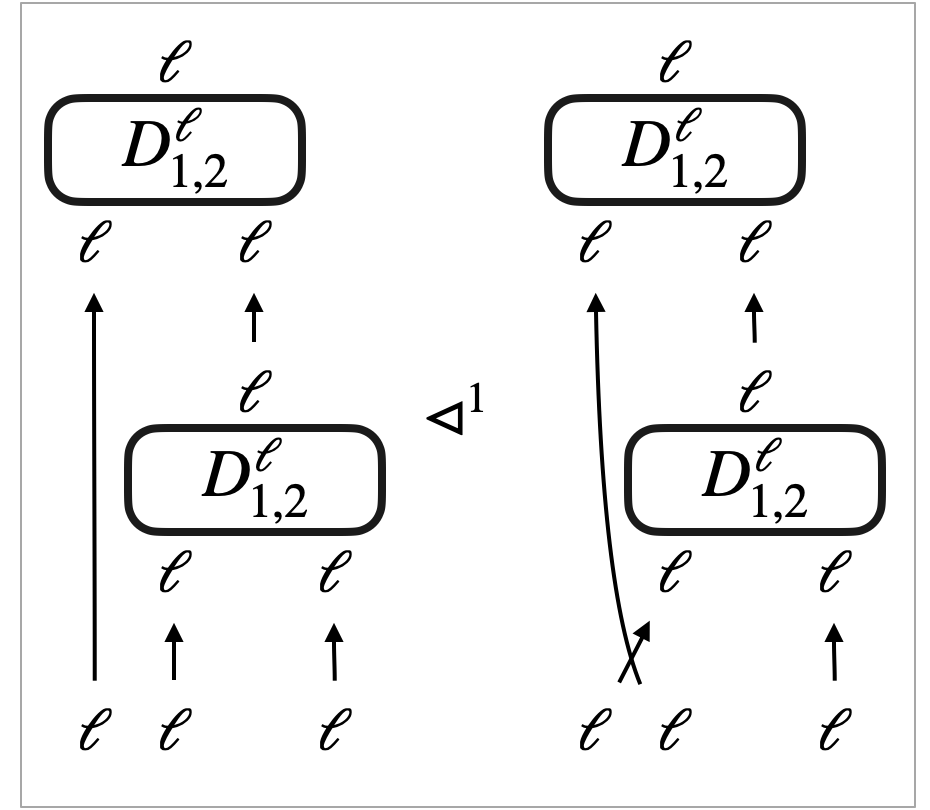 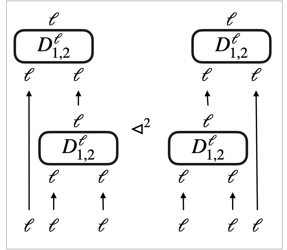 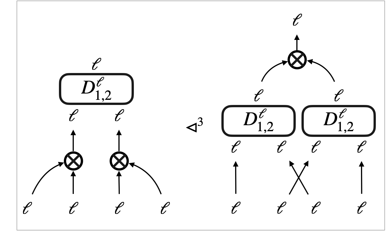
|
||
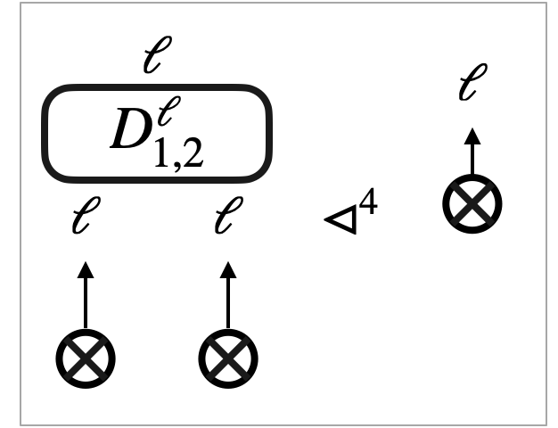 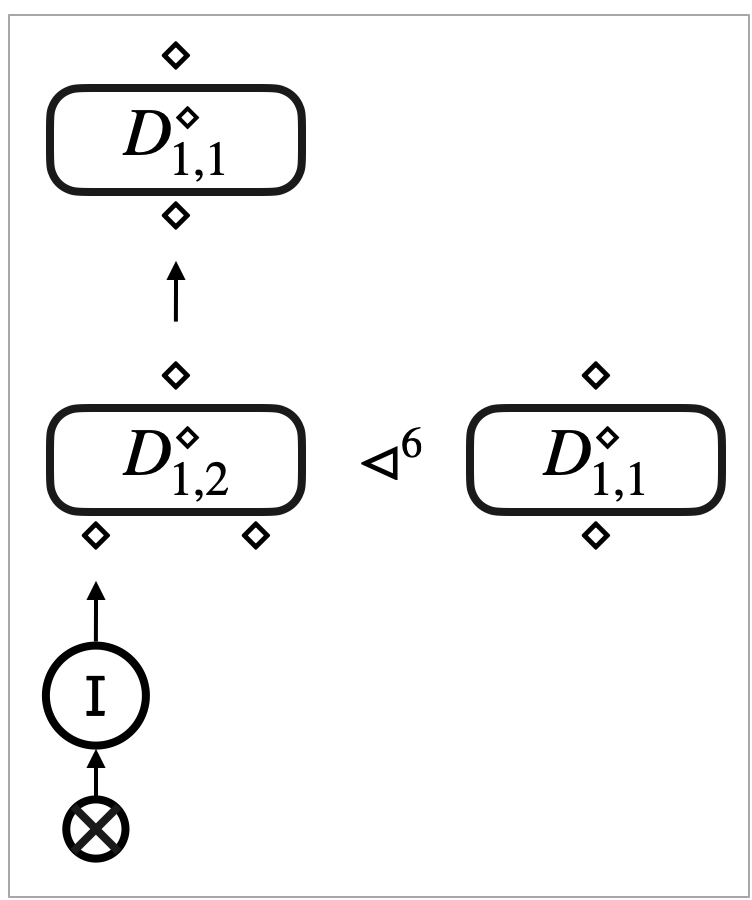 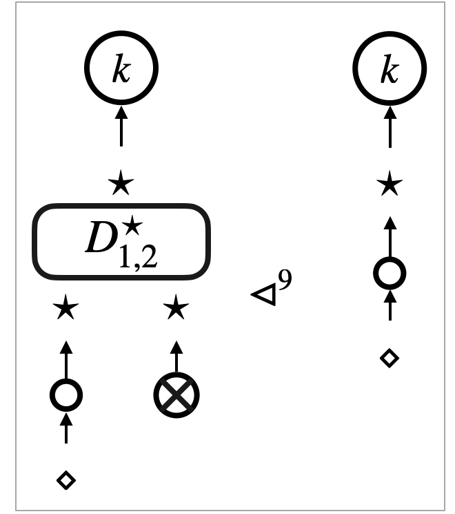
|
| dependency | implication of | used for | |
|---|---|---|---|
In this section we give some details of proving input-safety and robustness of the pre-templates for the Parametricity law, as indicated in Table 3. The proofs exploit the transfer properties established in 47.
Figure 24 lists triggers that we use to prove input-safety and robustness of some of the pre-templates777The numbering of triggers is according to the one used in [Mur20, Section 4.5.5]. Some of triggers in loc. cit. are for observational equivalences that we do not consider in this paper, and hence not presented here.. Table 5 shows contextual refinements/equivalences implied by these triggers (in the “implication” column), given that some pre-templates (shown in the “dependency” column) imply contextual refinement as shown in Table 3. All the implications can be proved simply using the congruence property and transitivity of contextual refinement. Table 5 shows which pre-template requires each trigger in its proof of input-safety or robustness (in the “used for” column). Note that the converse of any trigger is again a trigger.
Recall that there is a choice of contraction trees upon applying a contraction rule and some of the local rewrite rules. The minimum choice is to collect only contraction edges whose target is reachable from the token target. The maximum choice is to take the contraction tree(s) so that no contraction or weakening edge is incoming to the unique hole edge in a context.
H.3.1. Pre-templates on contraction trees
First we check input-safety and robustness of , and , which are all on contraction trees.
Input-safety of and can be checked as follows. Given a -specimen with an entering search token, because any input of a contraction tree is a source of a contraction edge, we have:
It can be observed that a rewrite transition is possible in if and only if a rewrite transition is possible in . When a rewrite transition is possible in both states, we can use 47(3), by considering a maximal possible contraction rule. The results of the rewrite transition can be given by a new quasi--specimen up to (here denotes equality on states). When no rewrite transition is possible, both of the states are not final but stuck.
H.3.2. Input-safety of pre-templates not on contraction trees
As mentioned in Section 12.2, pre-templates that relate hypernets with no input of type are trivially input-safety for any parameter . This leaves us pre-templates , , and to check.
As for , note that the pre-template relates hypernets with at least one input. Any -specimen of with an entering search token can be turned into the form where is a positive number. The proof is by case analysis on the number .
-
•
When , we have:
We can take as a -specimen, and the token in is not entering.
-
•
When , the token target must be a source of a contraction edge. There exist a focus-free context , two focus-free hypernets and a focus-free hypernet , such that
and given by the trigger via 42. The results of these sequences give a quasi--specimen up to .
A proof of input-safety of the operational pre-templates and is a simpler version of that of , because the operational pre-templates relate hypernets with only one input.
Let be either or . Any -specimen of an operational pre-template with an entering search token can be turned into the form ; note that the parameter that we had for is redundant in . We have:
We can take as a -specimen, and the token in is not entering. This data gives a -specimen when , which follows from the closedness of with respect to plugging (34). Note that can be seen as a context with no holes, which is trivially binding-free.
Finally, we look at the parametricity pre-template . Any -specimen of this pre-template, with an entering search token, can be turned into the form where is a positive number. The token target is a source of an edge labelled with , so we have:
The results of these sequences give a quasi--specimen up to .
H.3.3. Robustness of pre-templates not on contraction trees: a principle
Robustness can be checked by inspecting rewrite transition from the state given by a specimen of a pre-template, where the token of is not entering. We in particular consider the minimum local (contraction or rewrite) rule applied in this transition. This means that, in the hypernet , every vertex is reachable from the token target.
The inspection boils down to analyse how the minimum local rule involves edges that come from the hypernets . If all the involvement is deep, i.e. only deep edges from are involved in the local rule, these deep edges must come via deep holes in the context . We can use 47(1).
If the minimum local rule involves shallow edges that are from , endpoints of these edges are reachable from the token target. This means that, in the context , some holes are shallow and their sources are reachable from the token target. Moreover, given that the token is not entering in , the context has a path from the token target to a source of a hole edge.
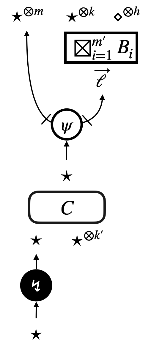
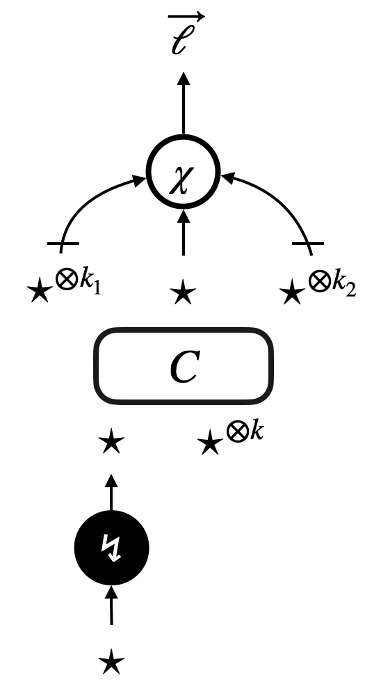
For example, in checking robustness of with respect to copy transitions, one situation of shallow overlaps is when is in the form in Figure 25a, and some of the box edges are from . Taking the minimum contraction rule means that in the graph is a contraction tree that gives a path from the token target. This path followed by the operation edge corresponds to paths from the token target to hole sources in the context .
So, if the minimum local rule involves shallow edges that are from , the context necessarily has a path from the token target to a hole source. The path becomes a path in the state , from the token target to a source of an edge that is from . The edge is necessarily shallow, and also involved in the application of the minimum local rule, because of the connectivity of . Moreover, a source of the edge is an input, in the relevant hypernet of . By inspecting minimum local rules, we can enumerate possible labelling of the path and the edge , as summarised in Table 6. Explanation on the notation used in the table is to follow.
| local rule | labels of path | label of edge |
|---|---|---|
| contraction | box | |
| box | ||
We use the regular-expression like notation in Table 6. For example, represents finite sequences of edge labels, where more than one occurrences of the label is followed by one operation . This characterises paths that inhabit the overlap shown in Figure 25a, i.e. the contraction tree followed by the operation edge . Note that this regular-expression like notation is not a proper regular expression, because it is over the infinite alphabet , the edge label set, and it accordingly admits infinite alternation (aka. union) implicitly.
H.3.4. Robustness of and its converse
Robustness check of the pre-template with respect to copy transitions has two cases. The first case is when one shallow overlap is caused by a path characterised by , and the second case is when no shallow overlaps are present and 47(1) can be used.
In the first case, namely, a -specimen with a non-entering rewrite token can be turned into the form where is a positive number, and is a focussed context in the form of Figure 25b. A rewrite transition is possible on both states given by the specimen, in which a contraction rule is applied to and . Results of the rewrite transition give a new quasi--specimen. When , this quasi-specimen is up to , using the trigger . When , the quasi-specimen is also up to , but using the trigger .
H.3.5. Robustness of and its converse
These two pre-templates both relate hypernets with no inputs. Proofs of their robustness always boil down to the use of 47(1), following the discussion in Section H.3.3. Namely, it is impossible to find the path in the context from the token target to a hole source.
H.3.6. Robustness of , and , and their converse
These six pre-templates all concern boxes. Using Table 6, shallow overlaps are caused by paths and from the token target.
As for compute transitions of the operation ‘’, either one path causes one shallow overlap, or all overlaps are deep. The latter situation boils down to 47(1). In the former situation, a micro-beta rule involves one box that is contributed by a pre-template, and states given by a -specimen are turned into a quasi--specimen up to , by one rewrite transition.
As for copy transitions, there are two possible situations.
-
•
Paths cause some shallow overlaps and there are some deep overlaps too.
- •
In the first situation, some of the shallow boxes duplicated by a contraction rule are contributed by a pre-template, and other duplicated boxes may have deep edges contributed by the pre-template. By tracking these shallow and deep contributions in a contraction rule, it can be checked that one rewrite transition turns states given by a -specimen into a quasi--specimen. This quasi-specimen is up to the following, depending on pre-templates:
-
•
for and its converse,
-
•
for , and for its converse, using the trigger , and
-
•
for , and for its converse, using the trigger .
H.3.7. Robustness of operational pre-templates and their converse
For the operational pre-templates and their converse, we use the class of binding-free contexts. This restriction is crucial to rule out some shallow overlaps.
Using Table 6, shallow overlaps with the operational pre-templates and are caused by paths from the token context. However, the restriction to binding-free contexts makes this situation impossible, which means the robustness check always boils down to 47(1) and 47(2).
In checking robustness of the converse and , shallow overlaps are caused by paths:
from the token target. Like the case of , all paths but give rise to a state that is not rooted, which can be checked using 41. The paths are impossible because of the binding-free restriction. As a result, this robustness check also boils down to 47(1) and 47(2).
H.3.8. Robustness of the parametricity pre-template and its converse
These two pre-templates concern lambda-abstractions, and they give rather rare examples of robustness check where we compare different numbers of transitions.
Using Table 6, shallow overlaps with these pre-templates are caused by paths:
from the token target.
As for compute transitions of operations , there are two possible situations.
-
•
Shallow overlaps are caused by paths or .
- •
In the first situation, a stable hypernet of a local rewrite rule (see e.g. Figure 19a) contains shallow edges, labelled with , that are contributed by a pre-template. The overlapped shallow contributions are not modified at all by the rewrite rule, and consequently, one rewrite transition results in a quasi--specimen up to .
As for copy transitions, either one path causes one shallow overlap, or all overlaps are deep. The latter situation boils down to 47(1). In the former situation, one lambda-abstraction contributed by a pre-template gets duplicated. Namely, a -specimen with a non-entering rewrite token can be turned into the form where is a focussed context in the form of Figure 25b. There exist a focussed context and two hypernets such that:
Results of these rewrite transitions give a new quasi--specimen up to .
As for compute transitions of the operation ‘’, there are two possible situations.
-
•
One path causes a shallow overlap of the edge that has label and gets eliminated by a micro-beta rewrite rule, and possibly some other paths cause shallow overlaps in the stable hypernet (see Figure 10b).
-
•
There are possibly deep overlaps, and paths may cause shallow overlaps in the stable hypernet .
In the second situation, all overlaps are not modified at all by the micro-beta rewrite rule, except for some deep overlaps turned shallow. Consequently, one rewrite transition results in a quasi--specimen up to .
In the first situation, one lambda-abstraction contributed by the pre-template is modified, while all the other shallow overlaps (if any) are not. We can focus on the lambda-abstraction. The micro-beta rewrite acts on the lambda-abstraction, an edge labelled with ‘’, and the stable hypernet .
The involved lambda-abstraction can be in two forms (see Figure 20). Firstly, it contains function application in its body. Application of the micro-beta rule discloses the inner function application, whose function side is another lambda-abstraction that can be related by the pre-template again. As a result, one rewrite transition yields a quasi--specimen up to . Secondly, the involved lambda-abstraction consists of dereferencing ‘’ or constant ‘’. Application of the micro-beta rule discloses the dereferencing, or constant, edge. When it is the dereferencing edge that is disclosed, the micro-beta rule is followed by a few transitions to perform dereferencing and produce the same constant ‘’. As a result, we compare nine transitions with one transition, and obtain a quasi--specimen up to , using triggers and .
The case of the converse of is similar. The only difference is that, in the last situation described above where we compare nine transitions with one transition and obtain a quasi--specimen up to , we obtain a quasi--specimen up to as a result of the symmetrical comparison of transitions.
On a final note, let us recall Section 12.4, where we observed some situations of robustness for using informal reduction semantics on terms. We namely observed situations where parts related by the pre-template is subject to the standard call-by-value beta reduction, either as an argument or a function. The involvement as a function corresponds to one of the robustness situations described in this section, namely: a shallow overlap with a micro-beta rewrite rule that is caused by a path and modified by the rewrite rule. The other involvement, which is as an argument, corresponds to a combination of two situations described in this section, namely: any overlaps with a contraction rule, and shallow overlaps with a micro-beta rule that are caused by paths and preserved. The combination is due to the fact that the universal abstraction machine decomposes the beta reduction into the micro-beta rewrite rule and contraction rules, making substitution explicit and not eager.