A robust lower order mixed finite element method for a strain gradient elasticity model

Mingqing Chen School of Mathematical Sciences, and MOE-LSC, Shanghai Jiao Tong University, Shanghai 200240, China mingqing_chen@sjtu.edu.cn , Jianguo Huang School of Mathematical Sciences, and MOE-LSC, Shanghai Jiao Tong University, Shanghai 200240, China jghuang@sjtu.edu.cn and Xuehai Huang School of Mathematics, Shanghai University of Finance and Economics, Shanghai 200433, China huang.xuehai@sufe.edu.cn

Abstract.

A robust nonconforming mixed finite element method is developed for a strain gradient elasticity (SGE) model. In two and three dimensional cases, a lower order $C^{0}$ -continuous $H^{2}$ -nonconforming finite element is constructed for the displacement field through enriching the quadratic Lagrange element with bubble functions. This together with the linear Lagrange element is exploited to discretize a mixed formulation of the SGE model. The robust discrete inf-sup condition is established. The sharp and uniform error estimates with respect to both the small size parameter and the Lamé coefficient are achieved, which is also verified by numerical results. In addition, the uniform regularity of the SGE model is derived under two reasonable assumptions.

Key words and phrases:

Strain gradient elasticity model, nonconforming mixed finite element method, regularity, robustness

2020 Mathematics Subject Classification:

65N12; 65N15; 65N22; 65N30;

The work of J. Huang was partially supported by NSFC (Grant No. 12071289) and the Fundamental Research Funds for the Central Universities. The work of X. Huang was partially supported by NSFC (Grant Nos. 12171300, 12071289), and the Natural Science Foundation of Shanghai (Grant No. 21ZR1480500).

1. Introduction

Size effect of microstructures at the nanoscale has been observed in many experiments. In order to account for such phenomenon, higher-order continuum theory has begun to emerge even since the early twentieth century. Unlike the classic continuum theory, the corresponding constitutive relations contain additional parameters to characterize the size of materials, giving rise to various elastic mathematical models (cf. [17, 54, 39, 28, 38, 2, 5, 46]). Historically, Cosserat brothers propose in their celebrated work [17] a continuum model concerning the effect of couple-stresses. Later on, Mindlin [38] develops a more general linear elasticity theory, but the associated model contains quite a number of size parameters. To make the balance between effective prediction and computation cost, Aifantis and his collaborators introduce in [5, 46] only one size parameter to produce a strain gradient elasticity (SGE) model for material deformation at the micro/nano scale. This SGE model is well accepted in engineering areas to deal with elastic-plastic problems. We refer the reader to the survey papers [7, 44] for details along this line. It is worth noting that for a microarchitecture or microstructure, if its separation of scales is not fully valid, such as pantographic [45, 4], lattice [26, 55] and cellular [27] metamaterials, one requires to invoke higher-order theory with many size parameters for mechanical computation. Moreover, homogenization methods are actively used to determine generalized material parameters (cf. [56, 22]).

Let $\Omega\subset\mathbb{R}^{d}$ ( $d=2,\,3$ ) be a bounded domain with Lipschitz boundary. The SGE model given in [5, 46] can be described as follows.

(1.1)

\begin{cases}-\operatorname{div}\big{(}(\bm{I}-\iota^{2}\Delta)\bm{\sigma}(\bm{u})\big{)}=\bm{f}&\textrm{ in }\Omega,\\ \bm{u}=\partial_{\bm{n}}\bm{u}=\bm{0}&\textrm{ on }\partial\Omega,\end{cases}

where $\bm{n}$ is the unit outward normal to $\partial\Omega$ , $\bm{u}=(u_{1},\ldots,u_{d})^{\intercal}$ is the displacement field, $\bm{f}$ is the applied force, $\bm{\sigma}(\bm{u})=2\mu\bm{\varepsilon}(\bm{u})+\lambda(\operatorname{div}\bm{u})\bm{I}$ , and $\bm{\varepsilon}(\bm{u})=(\varepsilon_{ij}(\bm{u}))_{d\times d}$ is the strain tensor field with $\varepsilon_{ij}(\bm{u})=1/2(\partial_{i}u_{j}+\partial_{j}u_{i}).$ Here $\lambda$ and $\mu$ are the Lamé constants, and $\bm{I}$ is the identity tensor field. The resulting stress field is given by $\tilde{\bm{\sigma}}(\bm{u})=(\bm{I}-\iota^{2}\Delta)\bm{\sigma}(\bm{u})$ , where $\iota\in(0,1)$ denotes the size parameter of the material under discussion. The SGE model (1.1) is a fourth order elliptic singular perturbation problem with small parameter $\iota$ , which will reduce to a second-order linear elasticity model (3.15) when $\iota=0$ . That means, the solution of the reduced problem would not meet one of the boundary conditions of problem (1.1), namely the value of the normal derivative on the boundary. This would lead to the phenomenon of boundary layer. Moreover, as $\lambda$ goes to infinity, one can see from (3.21) that $\|\operatorname{div}\bm{u}\|_{2}\to 0$ . In other words, with $\lambda$ becoming very large, the elastic material becomes nearly incompressible, and this would deteriorate the approximation accuracy of the lower-order conforming finite element methods and lead to the locking phenomenon. Hence, it is a very challenging issue to develop a robust numerical method with respect to both size parameter $\iota$ and Lamé constant $\lambda$ .

Finite element method (FEM) is a well-known numerical method for solving elastic problems. For example, many $C^{1}$ -conforming FEMs are used for solving strain gradient elasticity problems in two or three dimensions (cf. [3, 57, 58, 36, 42, 50, 52]). For avoiding higher order shape functions so as to alleviate the computational cost, many non-conforming FEMs are developed accordingly (cf. [49, 53, 59, 30, 31, 33, 32]). Another way is to use the mixed method, and in this case the displacement and stress fields can be approximated simultaneously (cf. [6, 11, 48, 43]).

More recently, the isogeometric analysis method has also been used for solving higher-order strain gradient models (cf. [8, 22, 25, 35, 40]). As far as we know, the method is first proposed by Hughes and his collaborators for solving various engineering problems (see [24, 19]), and the systematic error analysis is developed by Beirão da Veiga et al. in [9]. We mention that the optimal error estimates are obtained in some of the previous papers [8, 22, 40], but the parameter dependence is not considered theoretically there.

Now, let us review some existing results for error analysis of the SGE model (1.1). In [30, 31, 33, 32], Ming and his collaborators analyze several robust non-conforming FEMs with respect to the size parameter $\iota$ under some specific assumptions, but not robust with respect to the Lamé constant $\lambda$ . To fix this problem, as the Lamé system for the linear elasticity, they introduce a “pressure field” $p=\lambda\operatorname{div}\bm{u}$ to reformulate (1.1) in the form [34]

(1.2)

\begin{cases}-\operatorname{div}\big{(}(\bm{I}-\iota^{2}\Delta)(2\mu\bm{\varepsilon}(\bm{u}))\big{)}-\nabla\big{(}(\bm{I}-\iota^{2}\Delta)p\big{)}=\bm{f}&\textrm{ in }\Omega,\\ \operatorname{div}\bm{u}-\dfrac{1}{\lambda}p=0&\textrm{ in }\Omega,\\ \bm{u}=\partial_{\bm{n}}\bm{u}=\bm{0}&\textrm{ on }\partial\Omega.\end{cases}

And they propose lower order nonconforming finite element methods based on (1.2), and derived the robust error estimate of $\bm{u}_{0}-\bm{u}_{h}$ and $p_{0}-p_{h}$ in energy norm, rather than $\bm{u}-\bm{u}_{h}$ and $p-p_{h}$ , with respect to both Lamé constant $\lambda$ and size parameter $\iota$ under the assumption $\iota$ is much smaller than the mesh size $h$ . Here $(\bm{u}_{0},p_{0})$ is the solution of problem (1.2) with $\iota=0$ , i.e. the Lamé system. It is rather involved to acquire robust error estimate of $\bm{u}-\bm{u}_{h}$ and $p-p_{h}$ with respect to both Lamé constant $\lambda$ and size parameter $\iota$ , which motivates this paper. Besides, based on some assumptions of weak continuity, in his PhD thesis [51] supervised by Prof. Jun Hu, Tian constructed a family of robust nonconforming finite element methods with the reduced integration technique for the primal formulation of SGE model (1.1) in two dimensions.

In this paper we shall devise a robust nonconforming mixed finite element method based on (1.2) with respect to both the size parameter $\iota$ and the Lamé constant $\lambda$ . The well-posedness of problem (1.2) is related to the surjectivity of operator $\operatorname{div}:H_{0}^{1}(\Omega;\mathbb{R}^{d})\cap\iota H_{0}^{2}(\Omega;\mathbb{R}^{d})\to L_{0}^{2}(\Omega)\cap\iota H_{0}^{1}(\Omega)$ , which is equivalent to the inf-sup condition

(1.3)

\|q\|_{0}+\iota|q|_{1}\lesssim\sup_{\bm{v}\in H_{0}^{2}(\Omega;\mathbb{R}^{d})}\frac{(\operatorname{div}\bm{v},q)+\iota^{2}(\nabla\operatorname{div}\bm{v},\nabla q)}{|\bm{v}|_{1}+\iota|\bm{v}|_{2}}\quad\forall~{}q\in H_{0}^{1}(\Omega)\cap L_{0}^{2}(\Omega).

Here, the symbol $H_{0}^{1}(\Omega;\mathbb{R}^{d})\cap\iota H_{0}^{2}(\Omega;\mathbb{R}^{d})$ denotes the space $H_{0}^{2}(\Omega;\mathbb{R}^{d})$ equipped with norm $|\bm{v}|_{1}+\iota|\bm{v}|_{2}$ , while $L_{0}^{2}(\Omega)\cap\iota H_{0}^{1}(\Omega)$ denotes the space $H_{0}^{1}(\Omega)\cap L_{0}^{2}(\Omega)$ equipped with norm $\|q\|_{0}+\iota|q|_{1}$ . To develop robust finite element methods for problem (1.2), we need to find a pair of finite element spaces $V_{h}$ and $Q_{h}$ satisfying the discrete analogue of the inf-sup condition (1.3), where $V_{h}$ and $Q_{h}$ are used to discretize $H_{0}^{2}(\Omega;\mathbb{R}^{d})$ and $H_{0}^{1}(\Omega)\cap L_{0}^{2}(\Omega)$ , respectively. The smooth finite element de Rham complexes in [23, 14, 16] will ensure the discrete inf-sup condition, but suffer from large number of degrees of freedom (DoFs) and supersmooth DoFs. To this end, we construct a lower order $C^{0}$ -continuous $H^{2}$ -nonconforming finite element in two and three dimensions for the displacement field $\bm{u}$ , and use the continuous linear element to discretize the pressure field $p$ . The DoFs of the $H^{2}$ -nonconforming finite element involve

(\operatorname{div}\bm{v},q)_{F}\quad\forall~{}q\in\mathbb{P}_{0}(F),F\in\mathcal{F}(K),

which is vital to prove the robust discrete inf-sup condition with respect to the size parameter $\iota$ . With finite element spaces $V_{h}$ and $Q_{h}$ , we propose a robust nonconforming finite element method for problem (1.2). After establishing the discrete inf-sup condition and some interpolation error estimates, we achieve the robust error estimate $O(h^{1/2})$ of $\bm{u}-\bm{u}_{h}$ and $p-p_{h}$ with respect to both the size parameter $\iota$ and the Lamé constant $\lambda$ .

Another contribution of this work is building up the regularity of problem (1.1)

|\bm{u}-\bm{u}_{0}|_{1}+\iota\|\bm{u}\|_{2}+\iota^{2}\|\bm{u}\|_{3}+\lambda\|\operatorname{div}(\bm{u}-\bm{u}_{0})\|_{0}+\lambda\iota|\operatorname{div}\bm{u}|_{1}+\lambda\iota^{2}\|\operatorname{div}\bm{u}\|_{2}\lesssim\iota^{1/2}\|\bm{f}\|_{0},

under two reasonable assumptions. These assumptions are interesting problems in the field of partial differential equations. We prove the first assumption in two dimensions with the aid of the regularity of the triharmonic equation.

The rest of this paper is organized as follows. In Sect. 2, we recall some notations and existing results. Then the regularity result for SGE model is shown in Sect. 3. In Sect. 4, we construct a lower order $H^{2}$ -nonconforming finite element, and propose a mixed finite element method for SGE model. In Sect. 5, we derive the robust error estimates with respect to Lamé parameter $\lambda$ and size parameter $\iota$ . Finally, numerical examples are provided in Sect. 6.

2. Preliminaries

2.1. Notation and some basic inequalities

Throughout this paper, let $\Omega\subset\mathbb{R}^{d}$ ( $d=2,\,3$ ) be a convex polytope, which is partitioned into a family of shape regular simplices $\mathcal{T}_{h}=\{K\}$ ; $h_{K}={\rm diam}(K)$ and $h=\max_{K\in\mathcal{T}_{h}}h_{K}$ . Let $\mathcal{V}(\mathcal{T}_{h})$ and $\mathcal{V}^{i}(\mathcal{T}_{h})$ be the sets of all and interior vertices of $\mathcal{T}_{h}$ , respectively; denote by $\mathcal{E}(\mathcal{T}_{h})$ and $\mathcal{E}^{i}(\mathcal{T}_{h})$ (resp. $\mathcal{F}(\mathcal{T}_{h})$ and $\mathcal{F}^{i}(\mathcal{T}_{h})$ ) the sets of all and interior one-dimensional edges (resp. $(d-1)$ -dimensional faces) of $\mathcal{T}_{h}$ , respectively. When $d=2$ , it is evident that $\mathcal{F}(\mathcal{T}_{h})=\mathcal{E}(\mathcal{T}_{h})$ and $\mathcal{F}^{i}(\mathcal{T}_{h})=\mathcal{E}^{i}(\mathcal{T}_{h})$ . We next introduce the following macro elements for later requirement. For vertex $\delta\in\mathcal{V}(\mathcal{T}_{h})$ , edge $e\in\mathcal{E}(\mathcal{T}_{h})$ and face $F\in\mathcal{F}(\mathcal{T}_{h})$ , write $\omega_{\delta}$ , $\omega_{e}$ and $\omega_{F}$ to be respectively the unions of all simplices in $\mathcal{T}_{\delta}$ , $\mathcal{T}_{e}$ and $\mathcal{T}_{F}$ , where $\mathcal{T}_{\delta}$ , $\mathcal{T}_{e}$ and $\mathcal{T}_{F}$ is the set of all simplices in $\mathcal{T}_{h}$ sharing common vertex $\delta$ , edge $e$ and face $F$ respectively. In addition, for a finite set $A$ , denote by $\#A$ its cardinality. For all $F\in\mathcal{F}^{i}(\mathcal{T}_{h})$ , which are shared by two simplices $K^{+}$ and $K^{-}$ in $\mathcal{T}_{F}$ , denote by $\bm{n}$ the unit outward normal to $K^{+}$ and define the jump on $F$ as $\llbracket\partial_{\bm{n}}\bm{v}\rrbracket|_{F}\coloneqq\partial_{\bm{n}}\bm{v}|_{K_{+}}-\partial_{\bm{n}}\bm{v}|_{K_{-}}.$ We also write $\llbracket\partial_{\bm{n}}\bm{v}\rrbracket|_{F}\coloneqq\partial_{\bm{n}}\bm{v}|_{F}$ for all $F\in\mathcal{F}^{\partial}(\mathcal{T}_{h}):=\mathcal{F}(\mathcal{T}_{h})\backslash\mathcal{F}^{i}(\mathcal{T}_{h})$ .

Given a bounded domain $D\subset\mathbb{R}^{d}$ and integers $m,k\geq 0$ , denote by $H^{m}(D)$ the standard Sobolev space on $D$ with norm $\|\cdot\|_{m,D}$ and semi-norm $|\cdot|_{m,D}$ , and $H_{0}^{m}(D)$ the closure of $C_{0}^{\infty}(D)$ with respect to $\|\cdot\|_{m,D}$ . We abbreviate $\|\cdot\|_{m,\Omega}$ and $|\cdot|_{m,\Omega}$ as $\|\cdot\|_{m}$ and $|\cdot|_{m}$ respectively for $D=\Omega$ . The notation $(\cdot,\,\cdot)_{D}$ symbolizes the standard $L^{2}$ inner product on $D$ , and the subscript will be omitted when $D=\Omega$ . Let $\mathbb{P}_{k}(D)$ be the set of all polynomials on $D$ with the total degree up to $k$ . For a natural number $s$ , set $H^{m}(D;\mathbb{R}^{s}):=H^{m}(D)\otimes\mathbb{R}^{s}$ , $H_{0}^{m}(D;\mathbb{R}^{s}):=H_{0}^{m}(D)\otimes\mathbb{R}^{s}$ and $\mathbb{P}_{k}(D;\mathbb{R}^{s}):=\mathbb{P}_{k}(D)\otimes\mathbb{R}^{s}$ . Let $L^{2}_{0}(D)$ be the space of functions in $L^{2}(D)$ with vanishing integral average values.

For a scalar function $w$ and a vector valued function $\bm{v}=(v_{1},v_{2})^{\intercal}$ in two dimensions, introduce two usual differential operations $\operatorname{curl}w=(\partial_{2}w,-\partial_{1}w)^{\intercal}$ and $\operatorname*{rot}\bm{v}=\partial_{1}v_{2}-\partial_{2}v_{1}.$

As usual, we use $\lesssim$ to represent $\leq C$ , where $C$ may be a generic positive constant independent of the mesh size $h$ , the material parameter $\iota$ and the Lamé coefficient $\lambda$ . And $a\eqsim b$ indicates $a\lesssim b\lesssim a$ . Assume $\Omega$ is a star-shaped domain [12]. To deal with strain tensors, we need the first Korn’s inequality [12, Corollary 11.2.25]

(2.1)

\|\nabla\bm{v}\|_{0}\lesssim\|\bm{\varepsilon}(\bm{v})\|_{0}\quad\forall~{}\bm{v}\in H^{1}_{0}(\Omega;\mathbb{R}^{d}),

and the $H^{2}$ -Korn’s inequality [32, Theorem 1]

(2.2)

(1-1/\sqrt{2})|\bm{v}|_{2}^{2}\leq\|\nabla\bm{\varepsilon}(\bm{v})\|_{0}^{2}\quad\forall~{}\bm{v}\in H^{1}_{0}(\Omega;\mathbb{R}^{d})\cap H^{2}(\Omega;\mathbb{R}^{d}).

Recall the continuity of the right inverse of the divergence operator in [18].

Lemma 2.1.

For $p\in H_{0}^{m}(\Omega)\cap L_{0}^{2}(\Omega)$ with non-negative integer $m$ , there exists $\bm{v}\in H_{0}^{m+1}(\Omega;\mathbb{R}^{d})$ such that $\operatorname{div}\bm{v}=p$ and

\|\nabla\bm{v}\|_{j}\lesssim\|p\|_{j}\quad{\rm for}\;j=0,1,\ldots,m.

2.2. Mixed formulation

In order to solve the problem (1.1) with a mixed finite element method, we recall its mixed formulation in [34]. The variational formulation of (1.2) is to find $\bm{u}\in V:=H_{0}^{2}(\Omega;\mathbb{R}^{d})$ and $p\in Q:=H_{0}^{1}(\Omega)\cap L^{2}_{0}(\Omega)$ such that

(2.3)

\begin{cases}a(\bm{u},\bm{v})+b(\bm{v},p)=(\bm{f},\bm{v})&\forall~{}\bm{v}\in V,\\ b(\bm{u},q)-c(p,q)=0&\forall~{}q\in Q,\end{cases}

where

	$\displaystyle a(\bm{u},\bm{v})$	$\displaystyle:=2\mu(\bm{\varepsilon}(\bm{u}),\bm{\varepsilon}(\bm{v}))_{\iota}=2\mu\big{(}(\bm{\varepsilon}(\bm{u}),\bm{\varepsilon}(\bm{v}))+\iota^{2}(\nabla\bm{\varepsilon}(\bm{u}),\nabla\bm{\varepsilon}(\bm{v}))\big{)},$
	$\displaystyle b(\bm{v},p)$	$\displaystyle:=(\operatorname{div}\bm{v},p)_{\iota}=(\operatorname{div}\bm{v},p)+\iota^{2}(\nabla\operatorname{div}\bm{v},\nabla p),$
	$\displaystyle c(p,q)$	$\displaystyle:=(p,q)_{\iota}/\lambda=\big{(}(p,q)+\iota^{2}(\nabla p,\nabla q)\big{)}/\lambda$

with a weighted $H^{1}$ inner product $(p,q)_{\iota}:=(p,q)+\iota^{2}(\nabla p,\nabla q)$ . To make the forthcoming discussion in a compact way, we further introduce the following weighted Sobolev norms over $V$ and $Q$ :

\|\bm{v}\|_{V}:=\left(|\bm{v}|_{1}^{2}+\iota^{2}|\bm{v}|_{2}^{2}\right)^{1/2}\quad\forall\;\bm{v}\in V;\quad\|q\|_{Q}:=\left(\|q\|_{0}^{2}+\iota^{2}|q|_{1}^{2}\right)^{1/2}\quad\forall\;q\in Q.

Now, it is easy to check that the linear forms $a(\cdot,\cdot)$ , $b(\cdot,\cdot)$ and $c(\cdot,\cdot)$ are bounded on $V\times V$ , $V\times Q$ and $Q\times Q$ , respectively. The coercivity of the linear form $a(\cdot,\cdot)$ on $V\times V$ results from Korn’s inequalities (2.1)-(2.2). And the inf-sup condition

\|q\|_{Q}\lesssim\sup\limits_{\bm{v}\in V}\frac{b(\bm{v},q)}{\|\bm{v}\|_{V}}\quad\forall~{}q\in Q

holds from Lemma 2.1. Applying the Babuška-Brezzi theory [10], we have the stability

\|\bm{u}\|_{V}+\|p\|_{Q}\lesssim\sup_{\bm{v}\in V,\,q\in Q}\frac{a(\bm{u},\bm{v})+b(\bm{v},p)-b(\bm{u},q)+c(p,q)}{\|\bm{v}\|_{V}+\|q\|_{Q}}\quad\forall~{}\bm{u}\in V,p\in Q.

Therefore, the mixed formulation (2.3) is well-posed.

3. Some regularity estimates

In order to derive the robust error estimates for the proposed mixed finite element method in the next section, we require to develop a series of regularity estimates for the underlying (system of) partial differential equations. In fact, these results are interesting themselves.

Lemma 3.1.

If $\bm{f}\in H^{-2}(\Omega;\mathbb{R}^{d})$ , then the following problem

(3.1)

\begin{cases}\Delta^{2}\bm{\phi}+\nabla\Delta p=\bm{f}&{\rm in}\;\Omega,\\ \Delta\operatorname{div}\bm{\phi}=0&{\rm in}\;\Omega,\\ \bm{\phi}=\partial_{\bm{n}}\bm{\phi}=\bm{0}&{\rm on}\;\partial\Omega,\end{cases}

has a unique solution $(\bm{\phi},p)\in H_{0}^{2}(\Omega;\mathbb{R}^{d})\times(H_{0}^{1}(\Omega)\cap L_{0}^{2}(\Omega))$ such that

(3.2)

\|\bm{\phi}\|_{2}+\|p\|_{1}\lesssim\|\bm{f}\|_{-2}.

Proof.

It is routine that the weak formulation of problem (3.1) is to find $(\bm{\phi},p)\in H_{0}^{2}(\Omega;\mathbb{R}^{d})\times(H_{0}^{1}(\Omega)\cap L_{0}^{2}(\Omega))$ such that

(3.3)

\begin{cases}(\nabla^{2}\bm{\phi},\nabla^{2}\bm{\psi})+(\nabla\operatorname{div}\bm{\psi},\nabla p)=\langle\bm{f},\bm{\psi}\rangle&\forall~{}\bm{\psi}\in H_{0}^{2}(\Omega;\mathbb{R}^{d}),\\ (\nabla\operatorname{div}\bm{\phi},\nabla q)=0&\forall~{}q\in H_{0}^{1}(\Omega)\cap L_{0}^{2}(\Omega).\end{cases}

Clearly, the bilinear form $(\nabla^{2}\cdot,\nabla^{2}\cdot)$ is uniformly coercive over $H_{0}^{2}(\Omega;\mathbb{R}^{d})$ . On the other hand, thanks to Lemma 2.1, for every $q\in H_{0}^{1}(\Omega)\cap L_{0}^{2}(\Omega)$ , there exists a $\bm{\chi}\in H_{0}^{2}(\Omega;\mathbb{R}^{d})$ such that $q=\operatorname{div}\bm{\chi}$ which admits the estimate $\|\nabla\bm{\chi}\|_{1}\lesssim\|q\|_{1}$ . Hence,

\displaystyle\|q\|_{1}

\displaystyle\lesssim(\nabla q,\nabla q)/\|\nabla q\|_{0}\lesssim(\nabla\operatorname{div}\bm{\chi},\nabla q)/\|\nabla\bm{\chi}\|_{1}\lesssim\sup_{\bm{\psi}\in H_{0}^{2}(\Omega;\mathbb{R}^{d})}\frac{(\nabla\operatorname{div}\bm{\psi},\nabla q)}{\|\bm{\psi}\|_{2}}.

Thus, we conclude the desired result from the Babuška-Brezzi theory [10]. ∎

Next, we need to introduce two assumptions on the two auxiliary problems, which are the basis to develop subtle estimates for problem (1.1).

Assumption 3.1.

Assume that $\bm{f}\in H^{-1}(\Omega;\mathbb{R}^{d})$ . Let $(\bm{\phi},p)\in H_{0}^{2}(\Omega;\mathbb{R}^{d})\times(H_{0}^{1}(\Omega)\cap L_{0}^{2}(\Omega))$ be the solution of problem (3.1). Then $\bm{\phi}\in H^{3}(\Omega;\mathbb{R}^{d})$ and $p\in H^{2}(\Omega)$ which admit the estimate

(3.4)

\|\bm{\phi}\|_{3}+\|p\|_{2}\lesssim\|\bm{f}\|_{-1}.

We will prove Assumption 3.1 holds for a convex polygon in Section 3.1. Since the solution $\bm{\phi}$ of (3.3) is zero when $\bm{f}\in\nabla L^{2}(\Omega)$ , by replacing $\bm{f}$ in problem (3.1) with $\bm{f}+\nabla q$ , we have from (3.4) that

(3.5)

\|\bm{\phi}\|_{3}\lesssim\inf_{q\in L^{2}(\Omega)}\|\bm{f}+\nabla q\|_{-1}.

Assumption 3.2.

Assume that $\bm{f}\in H^{-1}(\Omega;\mathbb{R}^{d})$ . Let $\bm{u}\in H_{0}^{2}(\Omega;\mathbb{R}^{d})$ be the solution of the following problem:

\begin{cases}\Delta(\mathcal{L}\bm{u})=\bm{f}&{\rm in}\;\Omega,\\ \bm{u}=\partial_{\bm{n}}\bm{u}=\bm{0}&{\rm on}\;\partial\Omega,\end{cases}

where $\mathcal{L}\bm{u}=\mu\Delta\bm{u}+(\lambda+\mu)\nabla(\operatorname{div}\bm{u})$ is the usual Lamé operator, with $\lambda\in[0,\Lambda]$ and $\mu\in[\mu_{0},\mu_{1}]$ being the Lamé constants. Then $\bm{u}\in H^{3}(\Omega;\mathbb{R}^{d})$ and it admits the estimate

\|\bm{u}\|_{3}\lesssim\|\bm{f}\|_{-1},

where the hidden constant may depend on $\Lambda$ , $\mu_{0}$ and $\mu_{1}$ .

Remark 3.2.

If $\partial\Omega\in C^{\infty}$ , Assumption 3.2 holds in terms of the mathematical theory in [1]. However, if $\Omega$ is a polytope domain, as shown in [29], one should first figure out the operator pencil of the underlying problem and then discover the spectrum distribution in order to determine under which conditions Assumption 3.2 holds. Such study is rather involved, and we cannot ensure this assumption holds even for convex polygons until now.

3.1. Regularity results for triharmonic equations in two dimensions and applications

In this subsection, in view of the mathematical theory in [20, 29], we are going to develop the regularity theory for triharmonic equations with homogeneous boundary conditions over convex polygons. As far as we know, this result is new. It has its interest itself and will also be used to show Assumption 3.1 holds for a convex polygon in combination with some results in [18].

Before introducing and proving our regularity estimates, let us recall some existing results in [20]. As shown in Fig. 1, let $\Omega$ be a convex polygon with $X$ as a generic vertex which has an interior angle $\alpha\in(0,\pi)$ . Let $L$ be a strongly elliptic $2m$ -order differential operator defined on $\overline{\Omega}$ with constant coefficients, where $m$ is any given positive integer. Consider the following homogeneous Dirichlet boundary problem

(3.6)

\begin{cases}Lu=f&\text{in }\Omega,\\ u=\partial_{\bm{n}}u=\cdots=\partial_{\bm{n}}^{m-1}u=0&\text{on }\partial\Omega,\end{cases}

which induces the following operators for each positive real number $s$ :

	$\displaystyle L^{(s)}:H_{0}^{m}(\Omega)\cap H^{s+m}(\Omega)$	$\displaystyle\,\,\rightarrow\,\,H^{s-m}(\Omega),$
	$\displaystyle u{\,\,\,\,\,\,\,\,\,\,\,\,\,\,\,\,\,\,\,\,\,\,\,}$	$\displaystyle\,\,\rightarrow\,\,Lu.$

A key problem is to determine the regularity property of $L^{(s)}$ for $s>0$ .

Refer to caption — Figure 1. The schema of a polygonal vertex.

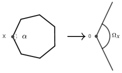
As a matter of fact, the problem can be answered locally. As shown in Fig. 1, for any given vertex $X$ , we might assume the unit circle $S_{X}$ centered at $X$ has intersection with each of two edges of $\Omega$ which share the vertex $X$ , and then write $\Omega_{X}=\Omega\cap S_{X}$ . Let $L_{X}$ be the principal part of $L$ . We introduce a polar coordinate system $(r,\theta)$ with $X$ as the origin. Then the differential operator $L_{X}$ can be expressed as

L_{X}(D_{\bm{x}})=r^{-2m}\mathcal{L}_{X}(\theta;r\partial_{r},D_{\theta}),

where $D_{\bm{x}}=\frac{1}{{\rm i}}\partial_{\bm{x}}$ , $D_{\theta}=\frac{1}{{\rm i}}\partial_{\theta}$ . Next, we replace $r\partial_{r}$ by a complex variable $\lambda\in\mathbb{C}$ , so as to get a holomorphic operator $\mathcal{L}_{X}(\lambda)=\mathcal{L}_{X}(\theta;\lambda,D_{\theta})$ which acts from $H^{m}_{0}(\Omega_{X})\cap H^{s+m}(\Omega_{X})$ into $H^{s-m}(\Omega_{X})$ . $\mathcal{L}_{X}(\lambda)$ is simply written as $\mathcal{L}(\lambda)$ when there is no confusion caused.

As shown in [20], the angle singularities of solution of elliptic equations have very close relationship with spectrum properties of $\mathcal{L}(\lambda)$ . Recall that a point $\lambda_{0}\in\mathbb{C}$ is said to be regular if the operator $\mathcal{L}(\lambda_{0})$ is invertible. The set of all non-regular points is called the spectrum of the operator. Then, by the well-known Peetre’s theorem and the main theorem in [20, p. 10] we can have a simplified result from [20], described as follows.

Theorem 3.3 (Dauge).

Let $\Omega$ be a convex polygon and let $L$ be a strongly elliptic $2m$ -order differential operator defined on $\overline{\Omega}$ with constant coefficients. Assume that the boundary value problem (3.6) has a unique solution $u\in H^{m}_{0}(\Omega)$ . Moreover, $s\geq 0$ and $s\not=\{\frac{1}{2},\frac{3}{2},\cdots,m-\frac{1}{2}\}$ . If any $\lambda\in\mathbb{C}$ with ${\rm Re}\lambda\in[m-1,s+m-1]$ is not spectrum of $\mathcal{L}(\lambda)$ and $f\in H^{s-m}(\Omega)$ , then $u\in H^{s+m}(\Omega)$ , and it holds the estimate

\|u\|_{s+m}\lesssim\|f\|_{s-m}.

On the other hand, it is rather involved to figure out the closed-form of $\mathcal{L}(\lambda)$ and analyze its spectrum distribution. However, it is very lucky that for the differential operator $L=(-\Delta)^{m}$ , we have from [29, Chapter 8] that

\mathcal{L}(\lambda)=(-1)^{m}\prod\limits_{j=0}^{m-1}(\partial_{\theta}^{2}+(\lambda-2j)^{2}),

and the following result holds.

Lemma 3.4.

[29, Chapter 8] If $\Omega$ is a convex polygon, and $L=(-\Delta)^{m}$ for a positive integer $m$ , then we have

(1)

the spectrum of $\mathcal{L}(\lambda)$ does not contain the points $m,\,m+1,\,\cdots\,,2m-1$ ;
(2)

the strip $m-2\leq{\rm Re}\lambda\leq m$ does not contain any eigenvalues of $\mathcal{L}(\lambda)$ .

Making use of the above two results, we can derive the regularity theory for the triharmonic equation given below.

Theorem 3.5.

Assume $\Omega$ is a convex polygon. Let $w\in H^{3}_{0}(\Omega)$ satisfy

(3.7)

-\Delta^{3}w=f\in H^{-2}(\Omega).

Then $w\in H^{4}(\Omega)$ and it admits the estimate

\|w\|_{4}\lesssim\|f\|_{-2}.

Proof.

The weak formulation of problem (3.7) is to find $w\in H_{0}^{3}(\Omega)$ such that

\int_{\Omega}\nabla^{3}w:\nabla^{3}v\,{\rm d}x=\langle f,v\rangle\quad\forall\;v\in H_{0}^{3}(\Omega).

Here, for any two third-order tensors $\bm{A}$ and $\bm{B}$ , $\bm{A}:\bm{B}=\sum_{ijk}A_{ijk}B_{ijk}$ , and $\langle\cdot,\cdot\rangle$ denotes the duality pair between $H^{-3}(\Omega)$ and $H_{0}^{3}(\Omega)$ . Hence, by the Poincaré inequality and the Lax-Milgram theorem, the last problem has a unique solution $w\in H_{0}^{3}(\Omega)$ . In other words, the boundary value problem (3.7) has a unique solution $w\in H_{0}^{3}(\Omega)$ for all $f\in H^{-3}(\Omega)$ . According to Lemma 3.4 with $m=3$ , $\mathcal{L}(\lambda)$ does not have a spectrum point in the strip $1\leq{\rm Re}\lambda\leq 3$ . Hence, we can conclude the desired result from Theorem 3.3 with $s=1$ . ∎

With the help of the above theorem, we can obtain the following result.

Theorem 3.6.

Assumption 3.1 holds whenever $\Omega$ is a convex polygon and $\bm{f}\in H^{-1}(\Omega;\mathbb{R}^{2})$ .

Proof.

Step 1: According to the second and third equations in (3.1), $\operatorname{div}\bm{\phi}\in H_{0}^{1}(\Omega)$ satisfies the Laplace equation, and hence $\operatorname{div}\bm{\phi}=0$ . Since $\bm{\phi}\in H_{0}^{2}(\Omega;\mathbb{R}^{2})$ , there exists a scalar function $w\in H^{3}_{0}(\Omega)$ [18] such that $\bm{\phi}=\operatorname{curl}w$ . Then apply the $\operatorname*{rot}$ operator to the first equality of (3.1) to get

-\Delta^{3}w=\operatorname*{rot}(\Delta^{2}\operatorname{curl}w)=\operatorname*{rot}(\Delta^{2}\bm{\phi})=\operatorname*{rot}(\Delta^{2}\bm{\phi}+\nabla\Delta p)=\operatorname*{rot}\bm{f}.

Due to Theorem 3.5, we know that $w\in H^{4}({\Omega})$ admits the estimate

\|w\|_{4}\lesssim\|\operatorname*{rot}\bm{f}\|_{-2}\lesssim\|\bm{f}\|_{-1}.

By the relation $\bm{\phi}=\operatorname{curl}w$ , we immediately have $\bm{\phi}\in H^{3}(\Omega;\mathbb{R}^{2})$ and

(3.8)

\|\bm{\phi}\|_{3}\lesssim\|\bm{f}\|_{-1}.

Step 2: Rewrite the first equation in (3.1) as $\nabla\Delta p=\bm{f}-\Delta^{2}\bm{\phi}.$ Since $\bm{f}-\Delta^{2}\bm{\phi}\in H^{-1}(\Omega;\mathbb{R}^{2})$ and $\Delta p\in H^{-1}(\Omega)$ , apply Theorem 2.2 in [21] to get $\Delta p\in L^{2}(\Omega)$ and

\|\Delta p\|_{0}\lesssim\|\Delta p\|_{-1}+\|\bm{f}-\Delta^{2}\bm{\phi}\|_{-1}\lesssim\|p\|_{1}+\|\bm{f}-\Delta^{2}\bm{\phi}\|_{-1},

which combined with (3.2) and (3.8) yields

\|\Delta p\|_{0}\lesssim\|\bm{f}\|_{-1}.

Noting that $\Omega$ is convex, by the regularity of Poisson’s equation,

\|p\|_{2}\lesssim\|\Delta p\|_{0}\lesssim\|\bm{f}\|_{-1}.

Now combining (3.8) and the last inequality gives (3.4). ∎

3.2. Regularity of the SGE model

Now we are ready to show the regularity results of the SGE model. From now on we always suppose Assumptions 3.1-3.2 hold.

Lemma 3.7.

Let $\bm{w}\in H_{0}^{2}(\Omega;\mathbb{R}^{d})$ be the solution of

(3.9)

\begin{cases}\operatorname{div}\Delta\big{(}2\mu\bm{\varepsilon}(\bm{w})+\lambda(\operatorname{div}\bm{w})\bm{I}\big{)}=\bm{f}&{\rm in}\;\Omega,\\ \bm{w}=\partial_{\bm{n}}\bm{w}=\bm{0}&{\rm on}\;\partial\Omega\end{cases}

with $\bm{f}\in H^{-1}(\Omega;\mathbb{R}^{d})$ . Suppose Assumptions 3.1-3.2 hold. We have

(3.10)		$\displaystyle\\|\bm{w}\\|_{2+j}+\lambda\\|\operatorname{div}\bm{w}\\|_{1+j}\lesssim\\|\bm{f}\\|_{j-2}\quad\textrm{ for }j=0,1,$
(3.11)		$\displaystyle\\|\bm{w}\\|_{3}\lesssim\inf_{q\in L^{2}(\Omega)}\\|\bm{f}+\nabla q\\|_{-1}+\frac{1}{\lambda}\\|\bm{f}\\|_{-1}.$

Proof.

We follow the argument of Lemma 2.2 in [13] to prove (3.10). The weak formulation of (3.9) is

(3.12)

2\mu(\nabla\bm{\varepsilon}(\bm{w}),\nabla\bm{\varepsilon}(\bm{v}))+\lambda(\nabla\operatorname{div}\bm{w},\nabla\operatorname{div}\bm{v})=(\bm{f},\bm{v})\quad\forall~{}\bm{v}\in H_{0}^{2}(\Omega;\mathbb{R}^{d}),

which is well-posed by the $H^{2}$ -Korn’s inequality (2.2), and it holds $\|\bm{w}\|_{2}\lesssim\|\bm{f}\|_{-2}.$ By Lemma 2.1, there exists $\widetilde{\bm{w}}\in H_{0}^{2}(\Omega;\mathbb{R}^{d})$ such that $\operatorname{div}\widetilde{\bm{w}}=\operatorname{div}\bm{w}$ and $\|\widetilde{\bm{w}}\|_{2}\lesssim\|\operatorname{div}\bm{w}\|_{1}.$ Taking $\bm{v}=\widetilde{\bm{w}}$ in (3.12), it follows that

\lambda|\operatorname{div}\bm{w}|_{1}^{2}=(\bm{f},\widetilde{\bm{w}})-2\mu(\nabla\bm{\varepsilon}(\bm{w}),\nabla\bm{\varepsilon}(\widetilde{\bm{w}}))\lesssim\|\bm{f}\|_{-2}\|\widetilde{\bm{w}}\|_{2}+\|\bm{w}\|_{2}\|\widetilde{\bm{w}}\|_{2},

which gives (3.10) for $j=0$ .

Next we prove (3.10) for $j=1$ . The first equation in (3.9) can be rewritten as

\Delta^{2}\bm{w}+\frac{\mu+\lambda}{\mu}\nabla\Delta\operatorname{div}\bm{w}=\frac{1}{\mu}\bm{f}\quad\textrm{ in }\Omega.

Clearly $\bm{w}\in H^{3}(\Omega;\mathbb{R}^{d})$ under Assumption 3.2. Employing lemma 2.1 again, there exists $\widetilde{\bm{w}}\in H^{3}(\Omega;\mathbb{R}^{d})\cap H_{0}^{2}(\Omega;\mathbb{R}^{d})$ such that $\operatorname{div}\widetilde{\bm{w}}=\operatorname{div}\bm{w}$ and $\|\widetilde{\bm{w}}\|_{3}\lesssim\|\operatorname{div}\bm{w}\|_{2}.$ With the help of $\widetilde{\bm{w}}$ , we have

\begin{cases}\Delta^{2}\bm{\phi}+\nabla\Delta p=\frac{1}{\mu}\bm{f}-\Delta^{2}\widetilde{\bm{w}}&\textrm{ in }\Omega,\\ \Delta\operatorname{div}\bm{\phi}=0&\textrm{ in }\Omega,\\ \bm{\phi}=\partial_{\bm{n}}\bm{\phi}=\bm{0}&\textrm{ on }\partial\Omega,\end{cases}

where $\bm{\phi}=\bm{w}-\widetilde{\bm{w}}$ and $p=\frac{\mu+\lambda}{\mu}\operatorname{div}\bm{w}$ . By (3.4)-(3.5),

(3.13)		$\displaystyle\\|\bm{w}-\widetilde{\bm{w}}\\|_{3}+\frac{\mu+\lambda}{\mu}\\|\operatorname{div}\bm{w}\\|_{2}$	$\displaystyle\lesssim\\|\bm{f}\\|_{-1}+\\|\widetilde{\bm{w}}\\|_{3},$
(3.14)		$\displaystyle\\|\bm{w}-\widetilde{\bm{w}}\\|_{3}$	$\displaystyle\lesssim\inf_{q\in L^{2}(\Omega)}\\|\bm{f}+\nabla q\\|_{-1}+\\|\widetilde{\bm{w}}\\|_{3}.$

By (3.13), there exists a constant $C>0$ such that

\|\bm{w}\|_{3}+\frac{\mu+\lambda}{\mu}\|\operatorname{div}\bm{w}\|_{2}\leq C(\|\bm{f}\|_{-1}+\|\operatorname{div}\bm{w}\|_{2}).

When $\lambda>2\mu C$ , i.e. $C<\frac{\lambda}{2\mu}$ , we get

\|\bm{w}\|_{3}+\frac{2\mu+\lambda}{2\mu}\|\operatorname{div}\bm{w}\|_{2}\leq C\|\bm{f}\|_{-1}.

Thus, (3.10) holds for $j=1$ . When $0<\lambda\leq 2\mu C$ , (3.10) for $j=1$ is guaranteed by Assumption 3.2.

It follows from (3.14) that

\|\bm{w}\|_{3}\lesssim\inf_{q\in L^{2}(\Omega)}\|\bm{f}+\nabla q\|_{-1}+\|\widetilde{\bm{w}}\|_{3}\lesssim\inf_{q\in L^{2}(\Omega)}\|\bm{f}+\nabla q\|_{-1}+\|\operatorname{div}\bm{w}\|_{2},

which together with (3.10) yields (3.11). ∎

Taking $\iota=0$ , problem (1.1) becomes the linear elasticity model. Let $\bm{u}_{0}\in H_{0}^{1}(\Omega;\mathbb{R}^{d})$ be the solution of the linear elasticity problem

(3.15)

\begin{cases}-\mu\Delta\bm{u}_{0}-(\lambda+\mu)\nabla\operatorname{div}\bm{u}_{0}=\bm{f}&\textrm{ in }\Omega,\\ \bm{u}_{0}=\bm{0}&\textrm{ on }\partial\Omega.\end{cases}

According to [13, 37], it holds

(3.16)

\|\bm{u}_{0}\|_{2}+\lambda\|\operatorname{div}\bm{u}_{0}\|_{1}\lesssim\|\bm{f}\|_{0}.

Lemma 3.8.

With the same assumptions as Lemma 3.7, let $\bm{u}\in H_{0}^{2}(\Omega;\mathbb{R}^{d})$ be the solution of problem (1.1), and $\bm{u}_{0}\in H_{0}^{1}(\Omega;\mathbb{R}^{d})$ satisfy the linear elasticity problem (3.15). It holds

(3.17)

|\bm{u}-\bm{u}_{0}|_{1}+\iota\|\bm{u}\|_{2}+\iota^{2}\|\bm{u}\|_{3}\lesssim\iota^{1/2}\|\bm{f}\|_{0}.

Proof.

By (1.1) and (3.15), we have

(3.18)

\operatorname{div}\Delta\bm{\sigma}(\bm{u})=\iota^{-2}\operatorname{div}\bm{\sigma}(\bm{u}-\bm{u}_{0}).

Then it follows from (3.11) that

	$\displaystyle\iota^{2}\\|\bm{u}\\|_{3}$	$\displaystyle\lesssim\inf_{q\in L^{2}(\Omega)}\\|\operatorname{div}\bm{\sigma}(\bm{u}-\bm{u}_{0})+\nabla q\\|_{-1}+\frac{1}{\lambda}\\|\operatorname{div}\bm{\sigma}(\bm{u}-\bm{u}_{0})\\|_{-1}$
(3.19)			$\displaystyle\lesssim\|\bm{u}-\bm{u}_{0}\|_{1}+\frac{1}{\lambda}\|\bm{u}-\bm{u}_{0}\|_{1}+\\|\operatorname{div}(\bm{u}-\bm{u}_{0})\\|_{0}\lesssim\|\bm{u}-\bm{u}_{0}\|_{1}.$

Multiply (3.18) by $\bm{u}-\bm{u}_{0}\in H^{2}(\Omega;\mathbb{R}^{d})\cap H_{0}^{1}(\Omega;\mathbb{R}^{d})$ and apply the integration by parts to get

	$\displaystyle\quad\iota^{2}(\nabla\bm{\sigma}(\bm{u}),\nabla\bm{\varepsilon}(\bm{u}))+(\bm{\sigma}(\bm{u}-\bm{u}_{0}),\bm{\varepsilon}(\bm{u}-\bm{u}_{0}))$
(3.20)		$\displaystyle=\iota^{2}(\nabla\bm{\sigma}(\bm{u}),\nabla\bm{\varepsilon}(\bm{u}_{0}))-\iota^{2}(\partial_{\bm{n}}\bm{\sigma}(\bm{u}),\bm{\varepsilon}(\bm{u}_{0}))_{\partial\Omega}.$

By (3.16),

	$\displaystyle(\nabla\bm{\sigma}(\bm{u}),\nabla\bm{\varepsilon}(\bm{u}_{0}))$	$\displaystyle=2\mu(\nabla\bm{\varepsilon}(\bm{u}),\nabla\bm{\varepsilon}(\bm{u}_{0}))+\lambda(\nabla\operatorname{div}\bm{u},\nabla\operatorname{div}\bm{u}_{0})$
		$\displaystyle\lesssim\|\bm{u}\|_{2}(\|\bm{u}_{0}\|_{2}+\lambda\|\operatorname{div}\bm{u}_{0}\|_{1})\lesssim\|\bm{u}\|_{2}\\|\bm{f}\\|_{0}.$

Applying the multiplicative trace inequality, (3.16) and (3.19),

	$\displaystyle-(\partial_{\bm{n}}\bm{\sigma}(\bm{u}),\bm{\varepsilon}(\bm{u}_{0}))_{\partial\Omega}$	$\displaystyle=-2\mu(\partial_{\bm{n}}\bm{\varepsilon}(\bm{u}),\bm{\varepsilon}(\bm{u}_{0}))_{\partial\Omega}-\lambda(\partial_{\bm{n}}\operatorname{div}\bm{u},\operatorname{div}\bm{u}_{0})_{\partial\Omega}$
		$\displaystyle\lesssim\\|\partial_{\bm{n}}\bm{\varepsilon}(\bm{u})\\|_{0,\partial\Omega}\\|\bm{\varepsilon}(\bm{u}_{0})\\|_{0,\partial\Omega}+\lambda\\|\partial_{\bm{n}}\operatorname{div}\bm{u}\\|_{0,\partial\Omega}\\|\operatorname{div}\bm{u}_{0}\\|_{0,\partial\Omega}$
		$\displaystyle\lesssim\\|\bm{u}\\|_{2}^{1/2}\\|\bm{u}\\|_{3}^{1/2}(\\|\bm{u}_{0}\\|_{2}+\lambda\\|\operatorname{div}\bm{u}_{0}\\|_{1})\lesssim\\|\bm{u}\\|_{2}^{1/2}\\|\bm{u}\\|_{3}^{1/2}\\|\bm{f}\\|_{0}$
		$\displaystyle\lesssim\iota^{-1}\\|\bm{u}\\|_{2}^{1/2}\\|\bm{f}\\|_{0}\|\bm{u}-\bm{u}_{0}\|_{1}^{1/2}.$

Combining the last two inequalities and (3.20) yields

	$\displaystyle\quad\iota^{2}(\nabla\bm{\sigma}(\bm{u}),\nabla\bm{\varepsilon}(\bm{u}))+(\bm{\sigma}(\bm{u}-\bm{u}_{0}),\bm{\varepsilon}(\bm{u}-\bm{u}_{0}))$
	$\displaystyle\lesssim\left(\iota^{3/2}\|\bm{u}\|_{2}+\iota^{1/2}\\|\bm{u}\\|_{2}^{1/2}\|\bm{u}-\bm{u}_{0}\|_{1}^{1/2}\right)\iota^{1/2}\\|\bm{f}\\|_{0}\lesssim\left(\iota\\|\bm{u}\\|_{2}+\|\bm{u}-\bm{u}_{0}\|_{1}\right)\iota^{1/2}\\|\bm{f}\\|_{0},$

which implies

\iota\|\bm{u}\|_{2}+|\bm{u}-\bm{u}_{0}|_{1}+\lambda^{1/2}\|\operatorname{div}(\bm{u}-\bm{u}_{0})\|_{0}+\lambda^{1/2}\iota|\operatorname{div}\bm{u}|_{1}\lesssim\iota^{1/2}\|\bm{f}\|_{0}.

Finally, we get (3.17) from (3.19). ∎

Theorem 3.9.

Let $\bm{u}\in H_{0}^{2}(\Omega;\mathbb{R}^{d})$ be the solution of problem (1.1), and $\bm{u}_{0}\in H_{0}^{1}(\Omega;\mathbb{R}^{d})$ satisfy the linear elasticity problem (3.15). Under the same assumptions as Lemma 3.7, it holds

(3.21)

\lambda\|\operatorname{div}(\bm{u}-\bm{u}_{0})\|_{0}+\lambda\iota|\operatorname{div}\bm{u}|_{1}+\lambda\iota^{2}\|\operatorname{div}\bm{u}\|_{2}\lesssim\iota^{1/2}\|\bm{f}\|_{0}.

Proof.

Applying Lemma 3.7 to (3.18), we obtain from (3.10) and (3.17) that

	$\displaystyle\lambda\iota^{2}\\|\operatorname{div}\bm{u}\\|_{2}$	$\displaystyle\lesssim\\|\operatorname{div}\bm{\sigma}(\bm{u}-\bm{u}_{0})\\|_{-1}\lesssim\\|\bm{\sigma}(\bm{u}-\bm{u}_{0})\\|_{0}\lesssim\|\bm{u}-\bm{u}_{0}\|_{1}+\lambda\\|\operatorname{div}(\bm{u}-\bm{u}_{0})\\|_{0}$
(3.22)			$\displaystyle\lesssim\iota^{1/2}\\|\bm{f}\\|_{0}+\lambda\\|\operatorname{div}(\bm{u}-\bm{u}_{0})\\|_{0}.$

Hence it suffices to prove

(3.23)

\lambda\|\operatorname{div}(\bm{u}-\bm{u}_{0})\|_{0}+\lambda\iota|\operatorname{div}\bm{u}|_{1}\lesssim\iota^{1/2}\|\bm{f}\|_{0}.

Thanks to Lemma 2.1, there exists $\bm{v}\in H^{2}(\Omega;\mathbb{R}^{d})\cap H_{0}^{1}(\Omega;\mathbb{R}^{d})$ such that

(3.24)

\operatorname{div}\bm{v}=\operatorname{div}(\bm{u}-\bm{u}_{0}),\quad\|\bm{v}\|_{1}\lesssim\|\operatorname{div}(\bm{u}-\bm{u}_{0})\|_{0}.

Multiply (3.18) by $\bm{v}$ and apply the integration by parts to get

	$\displaystyle\quad\lambda\\|\operatorname{div}(\bm{u}-\bm{u}_{0})\\|_{0}^{2}+\lambda\iota^{2}\|\operatorname{div}\bm{u}\|_{1}^{2}$
(3.25)		$\displaystyle=-2\mu(\bm{\varepsilon}(\bm{u}-\bm{u}_{0}),\bm{\varepsilon}(\bm{v}))+2\mu\iota^{2}(\Delta\bm{\varepsilon}(\bm{u}),\bm{\varepsilon}(\bm{v}))-\lambda\iota^{2}(\Delta\operatorname{div}\bm{u},\operatorname{div}\bm{u}_{0}).$

By the multiplicative trace inequality and (3.22), it holds

	$\displaystyle-\lambda\iota^{2}(\Delta\operatorname{div}\bm{u},\operatorname{div}\bm{u}_{0})$	$\displaystyle=\lambda\iota^{2}(\nabla\operatorname{div}\bm{u},\nabla\operatorname{div}\bm{u}_{0})-\lambda\iota^{2}(\partial_{\bm{n}}\operatorname{div}\bm{u},\operatorname{div}\bm{u}_{0})_{\partial\Omega}$
		$\displaystyle\lesssim\lambda\iota^{2}\|\operatorname{div}\bm{u}\|_{1}\|\operatorname{div}\bm{u}_{0}\|_{1}+\lambda\iota^{2}\|\operatorname{div}\bm{u}\|_{1}^{1/2}\\|\operatorname{div}\bm{u}\\|_{2}^{1/2}\\|\operatorname{div}\bm{u}_{0}\\|_{1}$
		$\displaystyle\lesssim\lambda\iota^{2}\|\operatorname{div}\bm{u}\|_{1}\|\operatorname{div}\bm{u}_{0}\|_{1}+\lambda^{1/2}\iota^{5/4}\|\operatorname{div}\bm{u}\|_{1}^{1/2}\\|\bm{f}\\|_{0}^{1/2}\\|\operatorname{div}\bm{u}_{0}\\|_{1}$
		$\displaystyle\quad+\lambda\iota\|\operatorname{div}\bm{u}\|_{1}^{1/2}\\|\operatorname{div}(\bm{u}-\bm{u}_{0})\\|_{0}^{1/2}\\|\operatorname{div}\bm{u}_{0}\\|_{1}.$

Then we acquire from (3.24)-(3.25) that

	$\displaystyle\quad\lambda\\|\operatorname{div}(\bm{u}-\bm{u}_{0})\\|_{0}^{2}+\lambda\iota^{2}\|\operatorname{div}\bm{u}\|_{1}^{2}$
	$\displaystyle\lesssim(\|\bm{u}-\bm{u}_{0}\|_{1}+\iota^{2}\|\bm{u}\|_{3})\|\bm{v}\|_{1}+\lambda\iota^{2}\|\operatorname{div}\bm{u}\|_{1}\|\operatorname{div}\bm{u}_{0}\|_{1}$
	$\displaystyle\quad+\lambda^{1/2}\iota^{5/4}\|\operatorname{div}\bm{u}\|_{1}^{1/2}\\|\bm{f}\\|_{0}^{1/2}\\|\operatorname{div}\bm{u}_{0}\\|_{1}+\lambda\iota\|\operatorname{div}\bm{u}\|_{1}^{1/2}\\|\operatorname{div}(\bm{u}-\bm{u}_{0})\\|_{0}^{1/2}\\|\operatorname{div}\bm{u}_{0}\\|_{1}$
	$\displaystyle\lesssim(\|\bm{u}-\bm{u}_{0}\|_{1}+\iota^{2}\|\bm{u}\|_{3})\\|\operatorname{div}(\bm{u}-\bm{u}_{0})\\|_{0}+(\lambda\iota^{2}\|\operatorname{div}\bm{u}\|_{1}^{2})^{1/2}(\lambda\iota^{2}\\|\operatorname{div}\bm{u}_{0}\\|_{1}^{2})^{1/2}$
	$\displaystyle\quad+\iota^{3/2}\|\operatorname{div}\bm{u}\|_{1}\\|\bm{f}\\|_{0}+\lambda\iota\\|\operatorname{div}\bm{u}_{0}\\|_{1}^{2}$
	$\displaystyle\quad+(\lambda\iota\|\operatorname{div}\bm{u}\|_{1}\\|\operatorname{div}(\bm{u}-\bm{u}_{0})\\|_{0})^{1/2}(\lambda\iota\\|\operatorname{div}\bm{u}_{0}\\|_{1}^{2})^{1/2}.$

This implies

\displaystyle\quad\lambda\|\operatorname{div}(\bm{u}-\bm{u}_{0})\|_{0}^{2}+\lambda\iota^{2}|\operatorname{div}\bm{u}|_{1}^{2}\lesssim\frac{1}{\lambda}(|\bm{u}-\bm{u}_{0}|_{1}+\iota^{2}|\bm{u}|_{3})^{2}+\lambda\iota\|\operatorname{div}\bm{u}_{0}\|_{1}^{2}+\frac{1}{\lambda}\iota\|\bm{f}\|_{0}^{2},

i.e.,

\lambda\|\operatorname{div}(\bm{u}-\bm{u}_{0})\|_{0}+\lambda\iota|\operatorname{div}\bm{u}|_{1}\lesssim|\bm{u}-\bm{u}_{0}|_{1}+\iota^{2}|\bm{u}|_{3}+\lambda\iota^{1/2}\|\operatorname{div}\bm{u}_{0}\|_{1}+\iota^{1/2}\|\bm{f}\|_{0}.

Therefore, we conclude (3.23) from (3.17) and (3.16). ∎

4. Mixed finite element method

In this section we will construct a lower order $C^{0}$ -continuous $H^{2}$ -nonconforming finite element, and apply to discretize the variational formulation (2.3) of SGE model (1.2).

4.1. $H^{2}$ -nonconforming finite element

For a $d$ -dimensional simplex $K$ ( $d=2,\,3$ ) with vertices $a_{1},\ldots,a_{d+1}$ , let $\mathcal{V}(K)$ , $\mathcal{E}(K)$ and $\mathcal{F}(K)$ be the sets of all vertices, one-dimensional edges and $(d-1)$ -dimensional faces of $K$ respectively. Set $\mathcal{V}^{i}(K):=\mathcal{V}(K)\cap\mathcal{V}^{i}(\mathcal{T}_{h})$ . For $s=1,\ldots,d+1$ , denote by $\lambda_{s}$ the barycentric coordinate corresponding to $a_{s}$ and there exists $F_{s}\in\mathcal{F}(K)$ such that $\lambda_{s}|_{F_{s}}=0$ . Let $b_{K}=\prod_{s=1}^{d+1}\lambda_{s}=\lambda_{j}b_{F_{j}}$ be the bubble function of $K$ , where $b_{F_{j}}$ is the bubble function of $F_{j}$ with $j=1,\cdots,d+1$ .

Given a face $F\in\mathcal{F}(K)$ with unit normal vector $\bm{n}$ , for a vector function $\bm{v}$ , define the tangential component $\Pi_{F}\bm{v}=\bm{v}-(\bm{v}\cdot\bm{n})\bm{n}$ . Then

(4.1)

\operatorname{div}\bm{v}=\operatorname{div}((\bm{v}\cdot\bm{n})\bm{n}+\Pi_{F}\bm{v})=\partial_{\bm{n}}(\bm{v}\cdot\bm{n})+\operatorname{div}_{F}\bm{v},

where face divergence $\operatorname{div}_{F}\bm{v}:=\operatorname{div}(\Pi_{F}\bm{v})$ .

With previous preparation, take

V(K):=\mathbb{P}_{2}(K;\mathbb{R}^{d})+b_{K}\mathbb{P}_{1}(K;\mathbb{R}^{d})+b_{K}^{2}\mathbb{P}_{0}(K;\mathbb{R}^{d})

as the space of shape functions. Then

\dim V(K)=d{d+2\choose 2}+d(d+1)+d=\frac{1}{2}d(d+2)(d+3).

The degrees of freedom (DoFs) are chosen as

(4.2)	$\displaystyle\bm{v}(\delta)$	$\displaystyle\quad\forall~{}\delta\in\mathcal{V}(K),$
(4.3)	$\displaystyle\frac{1}{\|e\|}(\bm{v},\bm{q})_{e}$	$\displaystyle\quad\forall~{}\bm{q}\in\mathbb{P}_{0}(e;\mathbb{R}^{d}),e\in\mathcal{E}(K),$
(4.4)	$\displaystyle\frac{1}{\|F\|}(\partial_{\bm{n}}(\bm{v}\cdot\bm{t}_{i}),q)_{F}$	$\displaystyle\quad\forall~{}q\in\mathbb{P}_{0}(F),F\in\mathcal{F}(K),i=1,\ldots,d-1,$
(4.5)	$\displaystyle\frac{1}{\|F\|}(\operatorname{div}\bm{v},q)_{F}$	$\displaystyle\quad\forall~{}q\in\mathbb{P}_{0}(F),F\in\mathcal{F}(K),$
(4.6)	$\displaystyle\frac{1}{\|K\|}(\bm{v},\bm{q})_{K}$	$\displaystyle\quad\forall~{}\bm{q}\in\mathbb{P}_{0}(K;\mathbb{R}^{d}),$

where $\bm{t}_{1},\ldots,\bm{t}_{d-1}$ are $(d-1)$ unit orthogonal tangential vectors of $F$ . DoF (4.5) is vital to prove the robust discrete inf-sup condition with respect to the size parameter $\iota$ .

Lemma 4.1.

The degrees of freedom (4.2)-(4.6) are uni-solvent for $V(K)$ .

Proof.

The number of the degrees of freedom (4.2)-(4.6) is

d(d+1)+d{d+1\choose 2}+d(d+1)+d=\frac{1}{2}d(d+2)(d+3)=\dim V(K).

Take $\bm{v}\in V(K)$ and assume all the degrees of freedom (4.2)-(4.6) vanish, then we prove $\bm{v}=\bm{0}$ . Noting that $\bm{v}|_{F}\in\mathbb{P}_{2}(F;\mathbb{R}^{d})$ for each $F\in\mathcal{F}(K)$ , we get from the vanishing DoFs (4.2)-(4.3) that $\bm{v}|_{\partial K}=\bm{0}$ . As a result there exist $\bm{v}_{1}\in\mathbb{P}_{1}(K;\mathbb{R}^{d})$ and $\bm{v}_{2}\in\mathbb{P}_{0}(K;\mathbb{R}^{d})$ such that $\bm{v}=b_{K}\bm{v}_{1}+b_{K}^{2}\bm{v}_{2}$ . Thanks to (4.1), the vanishing DoF (4.5) implies $(\partial_{\bm{n}}(\bm{v}\cdot\bm{n}),q)_{F}=0$ for all $q\in\mathbb{P}_{0}(F)$ , which combined with the vanishing DoF (4.4) yields $(\partial_{\bm{n}}\bm{v},\bm{q})_{F}=0$ for all $\bm{q}\in\mathbb{P}_{0}(F;\mathbb{R}^{d})$ , and thus

(b_{F}\bm{v}_{1},\bm{q})_{F}=0\quad\forall~{}\bm{q}\in\mathbb{P}_{0}(F;\mathbb{R}^{d}),F\in\mathcal{F}(K).

As a result $\bm{v}_{1}=\bm{0}$ . Finally, we conclude $\bm{v}=\bm{v}_{2}=\bm{0}$ from the vanishing DoF (4.6). ∎

Define a global $H^{2}$ -nonconforming finite element space:

	$\displaystyle V_{h}=$	$\displaystyle\{\bm{v}_{h}\in L^{2}(\Omega;\mathbb{R}^{d})\|\,\bm{v}_{h}\|_{K}\in V(K)\textrm{ for each }K\in\mathcal{T}_{h},\textrm{ all the DoFs \eqref{H2lowestncfemnDdof1}-\eqref{H2lowestncfemnDdof4}}$
		$\displaystyle\qquad\qquad\qquad\textrm{ are single-valued},\textrm{and DoFs \eqref{H2lowestncfemnDdof1}-\eqref{H2lowestncfemnDdof32} on boundary vanish}\}.$

Clearly $V_{h}\subset H_{0}^{1}(\Omega;\mathbb{R}^{d})$ , but $V_{h}\not\subset H^{2}(\Omega;\mathbb{R}^{d})$ . The finite element space $V_{h}$ has the weak continuity

(4.7)

\int_{F}\llbracket\nabla_{h}\bm{v}_{h}\rrbracket{\rm d}S=\bm{0}\quad\forall~{}\bm{v}_{h}\in V_{h},F\in\mathcal{F}(\mathcal{T}_{h}).

Here $\nabla_{h}$ is the elementwise version of $\nabla$ with respect to $\mathcal{T}_{h}$ .

Introduce the Lagrange element space $Q_{h}=Q_{h}^{L}\cap Q$ , where

Q_{h}^{L}:=\{q\in H^{1}(\Omega)\,|\,q|_{K}\in\mathbb{P}_{1}(K)\textrm{ for each }K\in\mathcal{T}_{h}\}.

Then the dicretization formulation of (2.3) is to find $(\bm{u}_{h},p_{h})\in V_{h}\times Q_{h}$ such that

(4.8)

\begin{cases}a_{h}(\bm{u}_{h},\bm{v}_{h})+b_{h}(\bm{v}_{h},p_{h})=(\bm{f},\bm{v}_{h})&\forall~{}\bm{v}_{h}\in V_{h},\\ b_{h}(\bm{u}_{h},q_{h})-c(p_{h},q_{h})=0&\forall~{}q_{h}\in Q_{h},\end{cases}

where

a_{h}(\bm{u}_{h},\bm{v}_{h}):=2\mu\big{(}(\bm{\varepsilon}(\bm{u}_{h}),\bm{\varepsilon}(\bm{v}_{h}))+\iota^{2}(\nabla_{h}\bm{\varepsilon}(\bm{u}_{h}),\nabla_{h}\bm{\varepsilon}(\bm{v}_{h}))\big{)},

b_{h}(\bm{v}_{h},p_{h}):=(\operatorname{div}\bm{v}_{h},p_{h})+\iota^{2}(\nabla_{h}\operatorname{div}\bm{v}_{h},\nabla p_{h}).

Define squared norm $\|\bm{v}_{h}\|^{2}_{V,h}:=|\bm{v}_{h}|_{1}^{2}+\iota^{2}|\bm{v}_{h}|_{2,h}^{2}$ with $|\bm{v}_{h}|_{2,h}^{2}=\sum_{K\in\mathcal{T}_{h}}|\bm{v}_{h}|_{2,K}^{2}.$ Clearly the discrete linear forms $a_{h}(\cdot,\cdot)$ and $b_{h}(\cdot,\cdot)$ are continuous on $V_{h}\times V_{h}$ and $V_{h}\times Q_{h}$ , respectively. Since $(1-1/\sqrt{2})|\bm{v}_{h}|_{2,h}^{2}\lesssim\|\nabla_{h}\bm{\varepsilon}(\bm{v}_{h})\|_{0}^{2}$ and the Korn’s inequality (2.1), we achieve the discrete coercivity

(4.9)

\|\bm{v}_{h}\|_{V,h}^{2}\lesssim a_{h}(\bm{v}_{h},\bm{v}_{h})\quad\forall~{}\bm{v}_{h}\in V_{h}.

4.2. Discrete inf-sup condition and uni-solvence

To derive the unisolvence of the mixed finite element method (4.8), we first introduce the second order Brezzi-Douglas-Marini (BDM) element [10, 15]. The second order BDM element takes $\mathbb{P}_{2}(K;\mathbb{R}^{d})$ as the shape function space, and the degrees of freedom are chosen as [15]

(4.10)		$\displaystyle(\bm{v}\cdot\bm{n},q)_{F}$	$\displaystyle\quad\forall~{}q\in\mathbb{P}_{2}(F),F\in\mathcal{F}(K),$
(4.11)		$\displaystyle(\bm{v},\bm{q})_{K}$	$\displaystyle\quad\forall~{}\bm{q}\in\mathbb{P}_{1}(K;\mathbb{R}^{d})\;{\rm satisfying}\;\bm{x}\cdot\bm{q}\in\mathbb{P}_{1}(K).$

Let $I_{K}^{BDM}:H^{1}(K;\mathbb{R}^{d})\to\mathbb{P}_{2}(K;\mathbb{R}^{d})$ be the nodal interpolation operator based on DoFs (4.10)-(4.11). It holds

(4.12)

\operatorname{div}(I_{K}^{BDM}\bm{v})=Q_{K}(\operatorname{div}\bm{v})\quad\forall~{}\bm{v}\in H^{1}(K;\mathbb{R}^{d}),

where $Q_{K}$ is the standard $L^{2}$ projection operator from $L^{2}(K)$ to $\mathbb{P}_{1}(K)$ . Let $I_{h}^{BDM}$ be the global version of $I_{K}^{BDM}$ .

Now we define interpolation operator $I_{h}:H_{0}^{2}(\Omega;\mathbb{R}^{d})\to V_{h}$ as follows:

	$\displaystyle(I_{h}\bm{v})(\delta)$	$\displaystyle=\frac{1}{\#\mathcal{T}_{\delta}}\sum_{K\in\mathcal{T}_{\delta}}(I_{K}^{BDM}\bm{v})(\delta),$
	$\displaystyle(I_{h}\bm{v},\bm{q})_{e}$	$\displaystyle=\frac{1}{\#\mathcal{T}_{e}}\sum_{K\in\mathcal{T}_{e}}(I_{K}^{BDM}\bm{v},\bm{q})_{e}\quad\forall~{}\bm{q}\in\mathbb{P}_{0}(e;\mathbb{R}^{d}),$
	$\displaystyle(\partial_{\bm{n}}(\Pi_{F}(I_{h}\bm{v})),\bm{q})_{F}$	$\displaystyle=\frac{1}{\#\mathcal{T}_{F}}\sum_{K\in\mathcal{T}_{F}}(\partial_{\bm{n}}(\Pi_{F}(I_{K}^{BDM}\bm{v})),\bm{q})_{F}\quad\forall~{}\bm{q}\in\mathbb{P}_{0}(F;\mathbb{R}^{d-1}),$
(4.13)		$\displaystyle(\operatorname{div}(I_{h}\bm{v}),q)_{F}$	$\displaystyle=\frac{1}{\#\mathcal{T}_{F}}\sum_{K\in\mathcal{T}_{F}}(\operatorname{div}(I_{K}^{BDM}\bm{v}),q)_{F}\quad\forall~{}q\in\mathbb{P}_{0}(F),$
(4.14)		$\displaystyle(I_{h}\bm{v},\bm{q})_{K}$	$\displaystyle=(\bm{v},\bm{q})_{K}\quad\forall~{}\bm{q}\in\mathbb{P}_{0}(K;\mathbb{R}^{d}),$

for $\delta\in\mathcal{V}^{i}(\mathcal{T}_{h})$ , $e\in\mathcal{E}^{i}(\mathcal{T}_{h})$ , $F\in\mathcal{F}^{i}(\mathcal{T}_{h})$ and $K\in\mathcal{T}_{h}$ .

Lemma 4.2.

We have

(4.15)		$\displaystyle\|I_{h}\bm{v}\|_{j,h}$	$\displaystyle\lesssim\|\bm{v}\|_{j}\quad\forall~{}\bm{v}\in H_{0}^{2}(\Omega;\mathbb{R}^{d}),j=1,2,$
(4.16)		$\displaystyle\sum_{i=0}^{3}h_{K}^{i}\|\bm{v}-I_{h}\bm{v}\|_{i,K}$	$\displaystyle\lesssim h_{K}^{3}\sum_{\delta\in\mathcal{V}(K)}\|\bm{v}\|_{3,\omega_{\delta}}\quad\forall~{}\bm{v}\in H_{0}^{2}(\Omega;\mathbb{R}^{d})\cap H^{3}(\Omega;\mathbb{R}^{d}).$

Proof.

Thanks to (4.11) and (4.14), it follows that

(I_{h}\bm{v}-I_{K}^{BDM}\bm{v},\bm{q})_{K}=0\quad\forall~{}\bm{q}\in\mathbb{P}_{0}(K;\mathbb{R}^{d}).

Then by the inverse inequality, scaling argument and (4.12),

		$\displaystyle h_{K}^{2i}\|I_{h}\bm{v}-I_{K}^{BDM}\bm{v}\|_{i,K}^{2}$
	$\displaystyle\lesssim$	$\displaystyle h_{K}^{d}\sum_{\delta\in\mathcal{V}(K)}(I_{h}\bm{v}-I_{K}^{BDM}\bm{v})^{2}(\delta)+h_{K}^{d-1}\sum_{e\in\mathcal{E}(K)}\\|I_{h}\bm{v}-I_{K}^{BDM}\bm{v}\\|_{0,e}^{2}$
		$\displaystyle+h_{K}^{3}\sum_{F\in\mathcal{F}(K)}\\|\partial_{\bm{n}}(\Pi_{F}(I_{h}\bm{v}-I_{K}^{BDM}\bm{v}))\\|_{0,F}^{2}+h_{K}^{3}\sum_{F\in\mathcal{F}(K)}\\|\operatorname{div}(I_{h}\bm{v}-I_{K}^{BDM}\bm{v})\\|_{0,F}^{2}$
	$\displaystyle\lesssim$	$\displaystyle h_{K}\sum_{\delta\in\mathcal{V}(K)}\sum_{F\in\mathcal{F}(T_{h}),\delta\in F}\\|\llbracket I_{K}^{BDM}\bm{v}\rrbracket\\|_{0,F}^{2}+h_{K}^{3}\sum_{F\in\mathcal{F}(K)}\\|\llbracket\partial_{\bm{n}}(I_{K}^{BDM}\bm{v})\rrbracket\\|_{0,F}^{2}$
		$\displaystyle+h_{K}^{3}\sum_{F\in\mathcal{F}(K)}\\|\llbracket Q_{K}(\operatorname{div}\bm{v})\rrbracket\\|_{0,F}^{2}.$

This implies

	$\displaystyle h_{K}^{2i}\|\bm{v}-I_{h}\bm{v}\|_{i,K}^{2}$	$\displaystyle\lesssim h_{K}^{2i}\|\bm{v}-I_{K}^{BDM}\bm{v}\|_{i,K}^{2}+h_{K}\sum_{\delta\in\mathcal{V}(K)}\sum_{F\in\mathcal{F}(T_{h}),\delta\in F}\\|\llbracket I_{K}^{BDM}\bm{v}\rrbracket\\|_{0,F}^{2}$
		$\displaystyle\quad+h_{K}^{3}\sum_{F\in\mathcal{F}(K)}\\|\llbracket\partial_{\bm{n}}(I_{K}^{BDM}\bm{v})\rrbracket\\|_{0,F}^{2}+h_{K}^{3}\sum_{F\in\mathcal{F}(K)}\\|\llbracket Q_{K}(\operatorname{div}\bm{v})\rrbracket\\|_{0,F}^{2}.$

Finally, we end the proof by employing the inverse inequality, the trace inequality, and the error estimates of $I_{K}^{BDM}$ and $Q_{K}$ . ∎

Next we present the discrete inf-sup condition.

Lemma 4.3.

It holds the discrete inf-sup condition

(4.17)

\|q_{h}\|_{Q}=\|q_{h}\|_{0}+\iota|q_{h}|_{1}\lesssim\sup_{\bm{v}_{h}\in\bm{V}_{h}}\frac{b_{h}(\bm{v}_{h},q_{h})}{\|\bm{v}_{h}\|_{V,h}}\quad\forall~{}q_{h}\in Q_{h}.

Proof.

By Lemma 2.1, there exists $\bm{v}\in H_{0}^{2}(\Omega;\mathbb{R}^{d})$ satisfying $\operatorname{div}\bm{v}=q_{h}$ and $|\bm{v}|_{1}+\iota|\bm{v}|_{2}\lesssim\|q_{h}\|_{0}+\iota|q_{h}|_{1}.$ Take $\bm{v}_{h}=I_{h}\bm{v}\in H_{0}^{1}(\Omega;\mathbb{R}^{d})$ . By (4.15),

(4.18)

|\bm{v}_{h}|_{1}+\iota|\bm{v}_{h}|_{2,h}\lesssim|\bm{v}|_{1}+\iota|\bm{v}|_{2}\lesssim\|q_{h}\|_{0}+\iota|q_{h}|_{1}.

For $K\in\mathcal{T}_{h}$ , by (4.12) and $\operatorname{div}\bm{v}\in Q_{h}$ , we have $\operatorname{div}(I_{K}^{BDM}\bm{v})=Q_{K}(\operatorname{div}\bm{v})=\operatorname{div}\bm{v}$ . Then we get from (4.13) and (4.14) that

	$\displaystyle(\operatorname{div}(\bm{v}_{h}-\bm{v}),q_{h})$	$\displaystyle=-(\bm{v}_{h}-\bm{v},\nabla q_{h})=0,$
	$\displaystyle(\nabla_{h}\operatorname{div}(\bm{v}_{h}-\bm{v}),\nabla q_{h})$	$\displaystyle=\sum_{K\in\mathcal{T}_{h}}(\operatorname{div}(\bm{v}_{h}-\bm{v}),\partial_{\bm{n}}q_{h})_{\partial K}=0.$

Combining the last two equations gives

b_{h}(\bm{v}_{h},q_{h})=(\operatorname{div}\bm{v},q_{h})+\iota^{2}(\nabla\operatorname{div}\bm{v},\nabla q_{h})=\|q_{h}\|_{0}^{2}+\iota^{2}|q_{h}|_{1}^{2},

which together with (4.18) ends the proof. ∎

Theorem 4.4.

It holds the discrete stability

(4.19)

\|\tilde{\bm{u}}_{h}\|_{V,h}+\|\tilde{p}_{h}\|_{Q}\lesssim\sup_{\bm{v}_{h}\in V_{h}\atop q_{h}\in Q_{h}}\frac{a_{h}(\tilde{\bm{u}}_{h},\bm{v}_{h})+b_{h}(\bm{v}_{h},\tilde{p}_{h})-b_{h}(\tilde{\bm{u}}_{h},q_{h})+c(\tilde{p}_{h},q_{h})}{\|\bm{v}_{h}\|_{V,h}+\|q_{h}\|_{Q}}

for $\tilde{\bm{u}}_{h}\in V_{h}$ and $\tilde{p}_{h}\in Q_{h}$ . Then the mixed finite element method (4.8) is well-posed.

Proof.

Applying the Babuška-Brezzi theory [10], we get from the discrete coercivity (4.9) and the discrete inf-sup condition (4.17) that

\|\tilde{\bm{u}}_{h}\|_{V,h}+\|\tilde{p}_{h}\|_{Q}\lesssim\sup_{\bm{v}_{h}\in V_{h},q_{h}\in Q_{h}}\frac{a_{h}(\tilde{\bm{u}}_{h},\bm{v}_{h})+b_{h}(\bm{v}_{h},\tilde{p}_{h})-b_{h}(\tilde{\bm{u}}_{h},q_{h})}{\|\bm{v}_{h}\|_{V,h}+\|q_{h}\|_{Q}}

for $\tilde{\bm{u}}_{h}\in V_{h}$ and $\tilde{p}_{h}\in Q_{h}$ , which indicates (4.19). ∎

5. Error analysis

We will analyze the mixed finite element method (4.8) in this section, and derive robust error estimates of $\|\bm{u}-\bm{u}_{h}\|_{V,h}+\|p-p_{h}\|_{Q}$ with respect to parameters $\iota$ and $\lambda$ .

5.1. Interpolation estimates

Denote by $I^{SZ}_{h}:H_{0}^{1}(\Omega)\to Q_{h}^{L}\cap H_{0}^{1}(\Omega)$ the Scott-Zhang interpolation operator with the homogeneous boundary condition [47]. Since $I^{SZ}_{h}v\not\in Q_{h}$ for $I^{SZ}_{h}v\not\in L_{0}^{2}(\Omega)$ , we will modify $I^{SZ}_{h}v$ .

For $K\in\mathcal{T}_{h}$ , let $N_{K}:=\#\mathcal{V}^{i}(K)$ be the number of interior vertices of $K$ . We assume the triangulation $\mathcal{T}_{h}$ satisfies $\min_{K\in\mathcal{T}_{h}}N_{K}\geq 1$ . Define operator $\mathcal{Q}_{h}:L^{2}(\Omega)\to Q_{h}^{L}\cap H_{0}^{1}(\Omega)$ by

(\mathcal{Q}_{h}v)(\delta)=\sum_{K\in\mathcal{T}_{\delta}}\frac{d+1}{N_{K}|\omega_{\delta}|}\int_{K}v~{}{\rm d}x\quad\forall~{}\delta\in\mathcal{V}^{i}(\mathcal{T}_{h}),

where $|\omega_{\delta}|$ is the geometrical measure of $\omega_{\delta}$ .

Lemma 5.1.

For $v\in L^{2}(\Omega)$ , we have $v-\mathcal{Q}_{h}v\in L_{0}^{2}(\Omega)$ , and

(5.1)

\|\mathcal{Q}_{h}v\|_{0,K}+h_{K}|\mathcal{Q}_{h}v|_{1,K}\lesssim\sum_{\delta\in\mathcal{V}^{i}(K)}\|v\|_{0,\omega_{\delta}}.

Proof.

By the fact $(\mathcal{Q}_{h}v)|_{K}\in\mathbb{P}_{1}(K)$ for $K\in\mathcal{T}_{h}$ ,

	$\displaystyle\quad\int_{\Omega}\mathcal{Q}_{h}v~{}{\rm d}x=\sum_{K\in\mathcal{T}_{h}}\int_{K}\mathcal{Q}_{h}v~{}{\rm d}x=\frac{1}{d+1}\sum_{K\in\mathcal{T}_{h}}\sum_{\delta\in\mathcal{V}^{i}(K)}\|K\|(\mathcal{Q}_{h}v)(\delta)$
	$\displaystyle=\frac{1}{d+1}\sum_{\delta\in\mathcal{V}^{i}(\mathcal{T}_{h})}\sum_{K\in\mathcal{T}_{\delta}}\|K\|(\mathcal{Q}_{h}v)(\delta)=\sum_{\delta\in\mathcal{V}^{i}(\mathcal{T}_{h})}\sum_{K\in\mathcal{T}_{\delta}}\sum_{K^{\prime}\in\mathcal{T}_{\delta}}\frac{\|K\|}{N_{K^{\prime}}\|\omega_{\delta}\|}\int_{K^{\prime}}v~{}{\rm d}x$
	$\displaystyle=\sum_{\delta\in\mathcal{V}^{i}(\mathcal{T}_{h})}\sum_{K^{\prime}\in\mathcal{T}_{\delta}}\frac{1}{N_{K^{\prime}}}\int_{K^{\prime}}v~{}{\rm d}x=\int_{\Omega}v~{}{\rm d}x.$

On the other side, by the scaling argument,

\|\mathcal{Q}_{h}v\|_{0,K}\lesssim h_{K}^{d/2}\sum_{\delta\in\mathcal{V}^{i}(K)}|(\mathcal{Q}_{h}v)(\delta)|\lesssim\sum_{\delta\in\mathcal{V}^{i}(K)}\|v\|_{0,\omega_{\delta}},

which together with the inverse inequality produces (5.1). ∎

Define $J_{h}:H_{0}^{1}(\Omega)\to Q_{h}^{L}\cap H_{0}^{1}(\Omega)$ by $J_{h}v:=I_{h}^{SZ}v+\mathcal{Q}_{h}(v-I_{h}^{SZ}v)$ . Since $\int_{\Omega}J_{h}v~{}{\rm d}x=\int_{\Omega}v~{}{\rm d}x$ , it holds that $J_{h}v\in Q_{h}$ when $v\in Q$ .

Lemma 5.2.

We have

(5.2)

h^{i}|v-J_{h}v|_{i}\lesssim h^{j}|v|_{j}\quad\forall~{}v\in H_{0}^{1}(\Omega)\cap H^{j}(\Omega),\;i\leq j\leq 2,\;i=0,1.

Proof.

For each $K\in\mathcal{T}_{h}$ , by (5.1) and $v-J_{h}v=v-I_{h}^{SZ}v-\mathcal{Q}_{h}(v-I_{h}^{SZ}v)$ ,

h_{K}^{i}|v-J_{h}v|_{i,K}\lesssim h_{K}^{i}|v-I_{h}^{SZ}v|_{i,K}+\sum_{\delta\in\mathcal{V}^{i}(K)}\|v-I_{h}^{SZ}v\|_{0,\omega_{\delta}}.

Therefore, we acquire (5.2) from the estimate of $I^{SZ}_{h}$ . ∎

To derive robust error estimates of $\|\bm{u}-\bm{u}_{h}\|_{V,h}+\|p-p_{h}\|_{Q}$ with respect to parameters $\iota$ and $\lambda$ , we introduce a finite element space

	$\displaystyle\tilde{V}_{h}:=$	$\displaystyle\{\bm{v}_{h}\in L^{2}(\Omega;\mathbb{R}^{d})\|\,\bm{v}_{h}\|_{K}\in V(K)\textrm{ for each }K\in\mathcal{T}_{h},\textrm{ all the DoFs \eqref{H2lowestncfemnDdof1}-\eqref{H2lowestncfemnDdof4}}$
		$\displaystyle\qquad\qquad\qquad\textrm{ are single-valued},\textrm{and DoFs \eqref{H2lowestncfemnDdof1}-\eqref{H2lowestncfemnDdof2} on boundary vanish}\}.$

Define an interpolation operator $\tilde{I}_{h}:H_{0}^{1}(\Omega;\mathbb{R}^{d})\to\tilde{V}_{h}$ as follows:

	$\displaystyle(\tilde{I}_{h}\bm{v})(\delta)$	$\displaystyle=\frac{1}{\#\mathcal{T}_{\delta}}\sum_{K\in\mathcal{T}_{\delta}}(I_{K}^{BDM}\bm{v})(\delta),$
	$\displaystyle(\tilde{I}_{h}\bm{v},\bm{q})_{e}$	$\displaystyle=\frac{1}{\#\mathcal{T}_{e}}\sum_{K\in\mathcal{T}_{e}}(I_{K}^{BDM}\bm{v},\bm{q})_{e}\quad\forall~{}\bm{q}\in\mathbb{P}_{0}(e;\mathbb{R}^{d}),$
	$\displaystyle(\partial_{\bm{n}}(\Pi_{F}(\tilde{I}_{h}\bm{v})),\bm{q})_{F}$	$\displaystyle=\frac{1}{\#\mathcal{T}_{F}}\sum_{K\in\mathcal{T}_{F}}(\partial_{\bm{n}}(\Pi_{F}(I_{K}^{BDM}\bm{v})),\bm{q})_{F}\quad\forall~{}\bm{q}\in\mathbb{P}_{0}(F;\mathbb{R}^{d-1}),$
	$\displaystyle(\operatorname{div}(\tilde{I}_{h}\bm{v}),q)_{F}$	$\displaystyle=\frac{1}{\#\mathcal{T}_{F}}\sum_{K\in\mathcal{T}_{F}}(\operatorname{div}(I_{K}^{BDM}\bm{v}),q)_{F}\quad\forall~{}q\in\mathbb{P}_{0}(F),$
	$\displaystyle(\tilde{I}_{h}\bm{v},\bm{q})_{K}$	$\displaystyle=(\bm{v},\bm{q})_{K}\quad\forall~{}\bm{q}\in\mathbb{P}_{0}(K;\mathbb{R}^{d}),$

for $\delta\in\mathcal{V}^{i}(\mathcal{T}_{h})$ , $e\in\mathcal{E}^{i}(\mathcal{T}_{h})$ , $F\in\mathcal{F}(\mathcal{T}_{h})$ and $K\in\mathcal{T}_{h}$ .

Lemma 5.3.

We have

(5.3)		$\displaystyle\|\tilde{I}_{h}\bm{v}\|_{1}$	$\displaystyle\lesssim\|\bm{v}\|_{1}\quad\forall~{}\bm{v}\in H_{0}^{1}(\Omega;\mathbb{R}^{d}),$
(5.4)		$\displaystyle\sum_{i=1}^{2}h_{K}^{i}\|\bm{v}-\tilde{I}_{h}\bm{v}\|_{i,K}$	$\displaystyle\lesssim h_{K}^{j}\sum_{\delta\in\mathcal{V}(K)}\|\bm{v}\|_{j,\omega_{\delta}}\;\forall~{}\bm{v}\in H_{0}^{1}(\Omega;\mathbb{R}^{d})\cap H^{j}(\Omega;\mathbb{R}^{d}),j=2,3.$

Proof.

Applying the similar argument as Lemma 4.2, we get for $i=1,2$ that

	$\displaystyle h_{K}^{2i}\|\tilde{I}_{h}\bm{v}-I_{K}^{BDM}\bm{v}\|_{i,K}^{2}\lesssim h_{K}\sum_{\delta\in\mathcal{V}(K)}\sum_{F\in\mathcal{F}(T_{h}),\delta\in F}\\|\llbracket I_{K}^{BDM}\bm{v}\rrbracket\\|_{0,F}^{2}$
(5.5)		$\displaystyle\qquad\qquad\quad+h_{K}^{3}\sum_{F\in\mathcal{F}^{i}(K)}\\|\llbracket\partial_{\bm{n}}(I_{K}^{BDM}\bm{v})\rrbracket\\|_{0,F}^{2}+h_{K}^{3}\sum_{F\in\mathcal{F}^{i}(K)}\\|\llbracket Q_{K}(\operatorname{div}\bm{v})\rrbracket\\|_{0,F}^{2}.$

Employing the inverse inequality, the trace inequality, the error estimates of $I_{K}^{BDM}$ and $Q_{K}$ ,

|\tilde{I}_{h}\bm{v}-I_{K}^{BDM}\bm{v}|_{1,K}\lesssim\sum_{\delta\in\mathcal{V}(K)}|\bm{v}|_{1,\omega_{\delta}},

which combined with the $H^{1}$ boundedness of $I_{K}^{BDM}$ yields (5.3).

On the other hand, by (5.5), we get

	$\displaystyle h_{K}^{2i}\|\bm{v}-\tilde{I}_{h}\bm{v}\|_{i,K}^{2}$	$\displaystyle\lesssim h_{K}^{2i}\|\bm{v}-I_{K}^{BDM}\bm{v}\|_{i,K}^{2}+h_{K}\sum_{\delta\in\mathcal{V}(K)}\sum_{F\in\mathcal{F}(T_{h}),\delta\in F}\\|\llbracket I_{K}^{BDM}\bm{v}\rrbracket\\|_{0,F}^{2}$
		$\displaystyle\quad+h_{K}^{3}\sum_{F\in\mathcal{F}^{i}(K)}\\|\llbracket\partial_{\bm{n}}(I_{K}^{BDM}\bm{v})\rrbracket\\|_{0,F}^{2}+h_{K}^{3}\sum_{F\in\mathcal{F}^{i}(K)}\\|\llbracket Q_{K}(\operatorname{div}\bm{v})\rrbracket\\|_{0,F}^{2}.$

Then (5.4) follows from the inverse inequality, the trace inequality, and the error estimates of $I_{K}^{BDM}$ and $Q_{K}$ . ∎

Lemma 5.4.

We have

(5.6)

|\bm{u}-\tilde{I}_{h}\bm{u}|_{1}+\iota|\bm{u}-\tilde{I}_{h}\bm{u}|_{2,h}\lesssim h^{1/2}\|\bm{f}\|_{0}.

Proof.

By (5.3)-(5.4) and (3.16)-(3.17),

\displaystyle|\bm{u}-\bm{u}_{0}-\tilde{I}_{h}(\bm{u}-\bm{u}_{0})|_{1}\lesssim h^{1/2}|\bm{u}-\bm{u}_{0}|_{1}^{1/2}|\bm{u}-\bm{u}_{0}|_{2}^{1/2}\lesssim h^{1/2}\|\bm{f}\|_{0}.

And it follows from (5.4) and (3.16) that

|\bm{u}_{0}-\tilde{I}_{h}\bm{u}_{0}|_{1}\lesssim h|\bm{u}_{0}|_{2}\lesssim h\|\bm{f}\|_{0}.

Combining the last two inequalities gives

|\bm{u}-\tilde{I}_{h}\bm{u}|_{1}\lesssim h^{1/2}\|\bm{f}\|_{0}.

According to (5.4) and (3.17), we have

|\bm{u}-\tilde{I}_{h}\bm{u}|_{2,h}\lesssim h^{1/2}|\bm{u}|_{2}^{1/2}|\bm{u}|_{3}^{1/2}\lesssim\iota^{-1}h^{1/2}\|\bm{f}\|_{0}.

Therefore, (5.6) holds from the last two inequalities. ∎

Lemma 5.5.

We have

(5.7)		$\displaystyle\|\bm{u}-I_{h}\bm{u}\|_{1}+\iota\|\bm{u}-I_{h}\bm{u}\|_{2,h}$	$\displaystyle\lesssim h^{1/2}\\|\bm{f}\\|_{0},$
(5.8)		$\displaystyle\\|p-J_{h}p\\|_{0}+\iota\|p-J_{h}p\|_{1}$	$\displaystyle\lesssim h^{1/2}\\|\bm{f}\\|_{0}.$

Proof.

We only prove (5.7), since the proof of (5.8) is similar. By the definitions of $I_{h}$ and $\tilde{I}_{h}$ , we get from the multiplicative trace inequality, the estimate of $I_{h}^{BDM}$ and (3.16)-(3.17) that

		$\displaystyle\|\tilde{I}_{h}\bm{u}-I_{h}\bm{u}\|_{1}^{2}\lesssim\sum_{F\in\mathcal{F}^{\partial}(\mathcal{T}_{h})}h_{F}\\|\nabla(\bm{u}-I_{h}^{BDM}\bm{u})\\|_{0,F}^{2}$
	$\displaystyle\lesssim$	$\displaystyle\sum_{F\in\mathcal{F}^{\partial}(\mathcal{T}_{h})}h_{F}\big{(}\\|\nabla(\bm{u}-\bm{u}_{0}-I_{h}^{BDM}(\bm{u}-\bm{u}_{0}))\\|_{0,F}^{2}+\\|\nabla(\bm{u}_{0}-I_{h}^{BDM}\bm{u}_{0})\\|_{0,F}^{2}\big{)}$
	$\displaystyle\lesssim$	$\displaystyle h\|\bm{u}-\bm{u}_{0}\|_{1}\|\bm{u}-\bm{u}_{0}\|_{2}+h^{2}\|\bm{u}_{0}\|_{2}^{2}\lesssim h\\|\bm{f}\\|_{0}^{2}.$

Similarly, we have

\displaystyle|\tilde{I}_{h}\bm{u}-I_{h}\bm{u}|_{2,h}^{2}

\displaystyle\lesssim\sum_{F\in\mathcal{F}^{\partial}(\mathcal{T}_{h})}h_{F}^{-1}\|\nabla(\bm{u}-I_{h}^{BDM}\bm{u})\|_{0,F}^{2}\lesssim h|\bm{u}|_{2}|\bm{u}|_{3}\lesssim\iota^{-2}h\|\bm{f}\|_{0}^{2}.

Hence

|\tilde{I}_{h}\bm{u}-I_{h}\bm{u}|_{1}+\iota|\tilde{I}_{h}\bm{u}-I_{h}\bm{u}|_{2,h}\lesssim h^{1/2}\|\bm{f}\|_{0}.

Finally, (5.7) holds from (5.6) and the last inequality. ∎

5.2. Error estimates

Similar to [41], we have the following abstract error estimates.

Lemma 5.6.

Let $(\bm{u},p)\in V\times Q$ and $(\bm{u}_{h},p_{h})\in V_{h}\times Q_{h}$ be the solution of problem (1.2) and problem (4.8), respectively. Then

\|\bm{u}-\bm{u}_{h}\|_{V,h}+\|p-p_{h}\|_{Q}\lesssim\inf_{\bm{u}_{I}\in V_{h}}\|\bm{u}-\bm{u}_{I}\|_{V,h}+\inf_{p_{I}\in Q_{h}}\|p-p_{I}\|_{Q}+E_{h},

where

E_{h}=\sup_{\bm{v}_{h}\in\bm{V}_{h}}\frac{(\bm{f},\bm{v}_{h})-a_{h}(\bm{u},\bm{v}_{h})-b_{h}(\bm{v}_{h},p)}{\|\bm{v}_{h}\|_{V,h}}.

Proof.

Let $\tilde{\bm{u}}_{h}=\bm{u}_{h}-\bm{u}_{I}$ and $\tilde{p}_{h}=p_{h}-p_{I}$ . It follows from the mixed finite element method (4.8) and the second equation of (2.3) that

		$\displaystyle a_{h}(\tilde{\bm{u}}_{h},\bm{v}_{h})+b_{h}(\bm{v}_{h},\tilde{p}_{h})-b_{h}(\tilde{\bm{u}}_{h},q_{h})+c(\tilde{p}_{h},q_{h})$
	$\displaystyle=$	$\displaystyle(\bm{f},\bm{v}_{h})-a_{h}(\bm{u}_{I},\bm{v}_{h})-b_{h}(\bm{v}_{h},p_{I})+b_{h}(\bm{u}_{I},q_{h})-c(p_{I},q_{h})$
	$\displaystyle=$	$\displaystyle(\bm{f},\bm{v}_{h})-a_{h}(\bm{u},\bm{v}_{h})-b_{h}(\bm{v}_{h},p)+a_{h}(\bm{u}-\bm{u}_{I},\bm{v}_{h})+b_{h}(\bm{v}_{h},p-p_{I})$
		$\displaystyle-b_{h}(\bm{u}-\bm{u}_{I},q_{h})+c(p-p_{I},q_{h}),$

which together with the discrete stability (4.19) ends the proof. ∎

Lemma 5.7.

We have

(5.9)		$\displaystyle E_{h}$	$\displaystyle\lesssim\iota h(\|\bm{u}\|_{3}+\lambda\|\operatorname{div}\bm{u}\|_{2}),$
(5.10)		$\displaystyle E_{h}$	$\displaystyle\lesssim h^{1/2}\\|\bm{f}\\|_{0}.$

Proof.

For $\bm{v}_{h}\in V_{h}\subset H_{0}^{1}(\Omega;\mathbb{R}^{d})$ , apply integration by parts to the first equation in problem (1.1) to acquire

		$\displaystyle(\bm{f},\bm{v}_{h})-a_{h}(\bm{u},\bm{v}_{h})-b_{h}(\bm{v}_{h},p)$
	$\displaystyle=$	$\displaystyle(\bm{\sigma}(\bm{u}),\bm{\varepsilon}(\bm{v}_{h}))-\iota^{2}(\Delta\bm{\sigma}(\bm{u}),\bm{\varepsilon}(\bm{v}_{h}))-a_{h}(\bm{u},\bm{v}_{h})-b_{h}(\bm{v}_{h},p)$
	$\displaystyle=$	$\displaystyle-\iota^{2}\sum\limits_{K\in\mathcal{T}_{h}}\int_{\partial K}\partial_{\bm{n}}\bm{\sigma}(\bm{u}):\bm{\varepsilon}(\bm{v}_{h}){\rm d}S.$

Let $Q_{F}^{0}$ be the standard $L^{2}$ -projection from $L^{2}(F)$ to $\mathbb{P}_{0}(F)$ , whose tensorial version is also denoted by $Q_{F}^{0}$ . By the weak continuity (4.7),

		$\displaystyle(\bm{f},\bm{v}_{h})-a_{h}(\bm{u},\bm{v}_{h})-b_{h}(\bm{v}_{h},p)$
	$\displaystyle=$	$\displaystyle-\iota^{2}\sum_{K\in\mathcal{T}_{h}}\sum_{F\in\mathcal{F}(K)}\int_{F}(\partial_{\bm{n}}\bm{\sigma}(\bm{u})-Q_{F}^{0}\partial_{\bm{n}}\bm{\sigma}(\bm{u})):(\bm{\varepsilon}(\bm{v}_{h})-Q_{F}^{0}\bm{\varepsilon}(\bm{v}_{h})){\rm d}S.$

From the error estimate of $Q_{F}^{0}$ and the trace inequality, we acquire

(\bm{f},\bm{v}_{h})-a_{h}(\bm{u},\bm{v}_{h})-b_{h}(\bm{v}_{h},p)\lesssim\iota^{2}h(|\bm{u}|_{3}+\lambda|\operatorname{div}\bm{u}|_{2})|\bm{v}_{h}|_{2,h},

(\bm{f},\bm{v}_{h})-a_{h}(\bm{u},\bm{v}_{h})-b_{h}(\bm{v}_{h},p)\lesssim\iota^{2}h^{1/2}(|\bm{u}|_{2}+\lambda|\operatorname{div}\bm{u}|_{1})^{1/2}(|\bm{u}|_{3}+\lambda|\operatorname{div}\bm{u}|_{2})^{1/2}|\bm{v}_{h}|_{2,h}.

Hence

E_{h}\lesssim\iota h(|\bm{u}|_{3}+\lambda|\operatorname{div}\bm{u}|_{2}),\quad E_{h}\lesssim\iota h^{1/2}(|\bm{u}|_{2}+\lambda|\operatorname{div}\bm{u}|_{1})^{1/2}(|\bm{u}|_{3}+\lambda|\operatorname{div}\bm{u}|_{2})^{1/2}.

Therefore, we finish the proof by using (3.17) and (3.21). ∎

Theorem 5.8.

Let $(\bm{u},p)\in(V\cap H^{3}(\Omega;\mathbb{R}^{d}))\times(Q\cap H^{2}(\Omega))$ and $(\bm{u}_{h},p_{h})\in V_{h}\times Q_{h}$ be the solution of problem (1.2) and (4.8), respectively. We have

(5.11)

\|\bm{u}-\bm{u}_{h}\|_{V,h}+\|p-p_{h}\|_{Q}\lesssim(h^{2}+\iota h)|\bm{u}|_{3}+\lambda(h^{2}+\iota h)|\operatorname{div}\bm{u}|_{2}.

Proof.

Let $\bm{u}_{I}=I_{h}\bm{u}\in V_{h}$ , and $p_{I}=J_{h}p\in Q_{h}$ in Lemma 5.6. Then by (4.16) and (5.2),

\|\bm{u}-\bm{u}_{h}\|_{V,h}+\|p-p_{h}\|_{Q}\lesssim(h^{2}+\iota h)|\bm{u}|_{3}+\lambda(h^{2}+\iota h)|\operatorname{div}\bm{u}|_{2}+E_{h}.

Therefore (5.11) follows from (5.9). ∎

Theorem 5.9.

With the same assumption of Theorem 5.8, we have

(5.12)		$\displaystyle\\|\bm{u}-\bm{u}_{h}\\|_{V,h}+\\|p-p_{h}\\|_{Q}$	$\displaystyle\lesssim h^{1/2}\\|\bm{f}\\|_{0},$
(5.13)		$\displaystyle\\|\bm{u}_{0}-\bm{u}_{h}\\|_{V,h}+\\|p_{0}-p_{h}\\|_{Q}$	$\displaystyle\lesssim(\iota^{1/2}+h^{1/2})\\|\bm{f}\\|_{0}.$

Proof.

The estimate (5.12) follows from Lemma 5.6, (5.7), (5.8) and (5.10). And estimate (5.13) holds from (5.12), (3.16)-(3.17) and (3.21). ∎

6. Numerical experiments

In this section, we present two numerical examples using the mixed FEM constructed in Sect 4.1 toward testifying its uniform convergence and robustness with respect to $\lambda$ and $\iota$ on a uniform triangulation.

To make the proposed method more accessible, we first present the mixed finite element spaces in two dimensions in detail. Let $\mathcal{T}_{h}$ be a shape regular triangulation. The finite element spaces in two dimensions are

	$\displaystyle V_{h}=$	$\displaystyle\{\bm{v}_{h}\in H_{0}^{1}(\Omega;\mathbb{R}^{2})\|\,\bm{v}_{h}\|_{K}\in V(K)\textrm{ for each }K\in\mathcal{T}_{h},\textrm{ all the DoFs \eqref{Ddof1}-\eqref{Ddof42}}$
		$\displaystyle\qquad\qquad\qquad\textrm{ are single-valued},\textrm{and DoFs \eqref{Ddof1}-\eqref{Ddof31} on boundary vanish}\},$
	$\displaystyle Q_{h}=$	$\displaystyle\{q_{h}\in H^{1}_{0}(\Omega)\cap L^{2}_{0}(\Omega)\,\|\,q_{h}\|_{K}\in\mathbb{P}_{1}(K)\textrm{ for each }K\in\mathcal{T}_{h}\},$

where $V(K)=\mathbb{P}_{2}(K;\mathbb{R}^{2})+b_{K}\mathbb{P}_{1}(K;\mathbb{R}^{2})+b_{K}^{2}\mathbb{P}_{0}(K;\mathbb{R}^{2})$ . The associated DoFs for $V_{h}$ are given as

(6.1)	$\displaystyle\bm{v}_{h}(\delta)$	$\displaystyle\quad\forall~{}\delta\in\mathcal{V}^{i}(\mathcal{T}_{h}),$
(6.2)	$\displaystyle\bm{v}_{h}(m_{e})$	$\displaystyle\quad\forall~{}e\in\mathcal{E}^{i}(\mathcal{T}_{h}),$
(6.3)	$\displaystyle\frac{1}{\|e\|}\int_{e}\partial_{\bm{n}}\bm{v}_{h}\,{\rm d}s$	$\displaystyle\quad\forall~{}e\in\mathcal{E}^{i}(\mathcal{T}_{h}),$
(6.4)	$\displaystyle\frac{1}{\|K\|}\int_{K}\bm{v}_{h}\,{\rm d}x$	$\displaystyle\quad\forall~{}K\in\mathcal{T}_{h},$

where $m_{e}$ is the midpoint of $e$ . The DoFs for $Q_{h}$ are all the function values at interior vertices. Note that the DoFs (6.1)-(6.3) on boundary vanish. The other point to be emphasized is that we here substitute DoFs (4.4)-(4.5) by the moments of the normal derivatives (6.3) owing to (4.1) in order to simplify computation. Also, we use the function values of midpoints on edges (6.2) instead of (4.3). With such substitution, the global finite element space remains the same.

Example 6.1.

Let $\Omega=(0,1)^{2}$ . We choose the right side function $\bm{f}$ such that the exact solution of SGE model (1.1) is

\displaystyle\bm{u}=

\displaystyle\begin{bmatrix}3(e^{\cos(2\pi x_{1})}-e)^{2}\sin(2\pi x_{2})\sin(\pi x_{2})\\ 8(e^{2\cos(2\pi x_{1})}-e^{1+\cos(2\pi x_{1})})\sin(2\pi x_{1})\sin^{3}(\pi x_{2})\end{bmatrix}.

Moreover, set $\mu=1$ . It is easy to check that $\bm{u}$ is divergence-free without boundary layer, and hence $\bm{f}$ is independent of the Lamé constant $\lambda$ . The purpose of this example is to demonstrate the error estimate given in Theorem 5.8.

We measure the relative error by

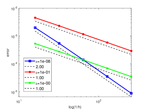
E_{u}\coloneqq\frac{\|\bm{u}-\bm{u}_{h}\|_{V,h}}{\|\bm{f}\|_{0}}.

The numerical results of $E_{u}$ are displayed in Table 1 with different values of Lamé constant $\lambda$ , size parameter $\iota$ and mesh size $h$ . We may observe from Table 1 that when $\iota$ takes the value $1$ and $1e-01$ , the relative error is linearly convergent and when $\iota=1e-08$ , it is quadratically convergent. In particular, Fig. 2 performs the relative error curves for different $\iota$ with fixed $\lambda=1e+08$ . In this situation, if $\iota=1e-08$ , $E_{u}$ behaves like $O(h^{2})$ . If $\iota=1e-01$ or $1e-00$ , $E_{u}=O(h)$ . Hence, we may conclude that the convergence order of the error is quadratic as $\iota\ll h$ . All these results are in good agreement with the error bound given in Theorem 5.8.

Table 1. The performance of Example 6.1.

$\lambda$	$\iota$	$h$					rate
$\lambda$	$\iota$	1/16	1/32	1/64	1/128	1/256	rate
1e+00	$1e-00$	5.375e-04	2.776e-04	1.399e-04	7.010e-05	3.507e-05	1.00
	$1e-01$	4.561e-03	2.334e-03	1.173e-03	5.874e-04	2.938e-04	1.00
	$1e-08$	2.008e-03	5.477e-04	1.407e-04	3.540e-05	8.862e-06	2.00
1e+04	$1e-00$	5.375e-04	2.776e-04	1.399e-04	7.010e-05	3.507e-05	1.00
	$1e-01$	4.562e-03	2.334e-03	1.173e-03	5.874e-04	2.938e-04	1.00
	$1e-08$	2.009e-03	5.477e-04	1.407e-04	3.540e-05	8.862e-06	2.00
1e+08	$1e-00$	5.375e-04	2.776e-04	1.399e-04	7.010e-05	3.507e-05	1.00
	$1e-01$	4.562e-03	2.334e-03	1.173e-03	5.874e-04	2.938e-04	1.00
	$1e-08$	2.009e-03	5.477e-04	1.407e-04	3.540e-05	8.862e-06	2.00

Table 2. The performance of Example 6.2.

$\lambda$	$\iota$	$h$					rate
$\lambda$	$\iota$	1/16	1/32	1/64	1/128	1/256	rate
1e+00	$1e-04$	2.053e-02	1.447e-02	1.025e-02	7.340e-03	5.438e-03	0.43
	$1e-06$	2.052e-02	1.445e-02	1.020e-02	7.206e-03	5.093e-03	0.50
	$1e-08$	2.052e-02	1.445e-02	1.020e-02	7.206e-03	5.093e-03	0.50
1e+04	$1e-04$	2.054e-02	1.447e-02	1.025e-02	7.341e-03	5.438e-03	0.43
	$1e-06$	2.053e-02	1.446e-02	1.020e-02	7.207e-03	5.094e-03	0.50
	$1e-08$	2.053e-02	1.446e-02	1.020e-02	7.207e-03	5.094e-03	0.50
1e+08	$1e-04$	2.054e-02	1.447e-02	1.025e-02	7.341e-03	5.438e-03	0.43
	$1e-06$	2.053e-02	1.446e-02	1.020e-02	7.207e-03	5.094e-03	0.50
	$1e-08$	2.053e-02	1.446e-02	1.020e-02	7.207e-03	5.094e-03	0.50

Example 6.2.

Let $\Omega=(0,1)^{2}$ . The exact solution of the reduced problem (3.15) is set to be a divergence-free function in the form

\displaystyle\bm{u}_{0}=

\displaystyle\begin{bmatrix}-x_{1}^{2}(1-x_{1})^{2}x_{2}(1-x_{2})(1-2x_{2})\\ x_{1}(1-x_{1})(1-2x_{1})x_{2}^{2}(1-x_{2})^{2}\end{bmatrix}.

The right side term $\bm{f}$ computed from (3.15) is independent of both $\lambda$ and $\iota$ . We use this $\bm{f}$ as the right side function of problem (1.1). Since $\partial_{\bm{n}}\bm{u}_{0}|_{\partial\Omega}\not=\bm{0}$ , the function $\bm{u}$ has a strong boundary layer when $\iota$ is sufficient small. We still set $\mu=1$ . We focus on investigating the robustness of our numerical method with respect to both $\lambda$ and $\iota$ in this example.

When $\iota\ll h$ , it follows from (3.16)-(3.17) and (3.21) that

\|\bm{u}-\bm{u}_{0}\|_{V}\lesssim\iota^{1/2}\|\bm{f}\|_{0}\lesssim h^{1/2}\|\bm{f}\|_{0},

which combined with (5.13) immediately implies (5.12). So we turn to verify the estimate (5.13), which depends on $\bm{u}_{0}$ instead of the unknown function $\bm{u}$ . Let $E_{u_{0}}=\frac{\|\bm{u}_{h}-\bm{u}_{0}\|_{V,h}}{\|\bm{f}\|_{0}}$ . We compute its values for different values of Lamé constant $\lambda$ and the mesh size $h$ in Table 2. We may observe that $E_{u_{0}}=O(h^{0.43})$ with $\iota=1e-04$ and $E_{u_{0}}=O(h^{1/2})$ with $\iota=1e-06$ or $1e-08$ no matter what value $\lambda$ takes. We can see that the best convergence order is really $1/2$ when $\iota\ll h$ , which is consistent with the estimate (5.13) and shows the robustness of the mixed finite element method with respect to both the size parameter $\iota$ and Lamé coefficient $\lambda$ .

Acknowledgments

The second author would like to thank Prof. M. Dauge from Université de Rennes 1 for helpful discussion about elliptic boundary value problems in domains with corners and bringing his attention to the monograph [29]. The authors are also indebted to the referees for valuable comments which improved an earlier version of the paper.

References

[1] S. Agmon, A. Douglis, and L. Nirenberg. Estimates near the boundary for solutions of elliptic partial differential equations satisfying general boundary conditions II. Commun. Pure. Appl. Math., 17:35–92, 02 1964.
[2] E. C. Aifantis. On the microstructural origin of certain inelastic models. J. Eng. Mater. Technol., 106(4):326–330, 1984.
[3] S. Akarapu and H. M. Zbib. Numerical analysis of plane cracks in strain-gradient elastic materials. Int. J. Fract., 141(3-4):403–430, 2006.
[4] J.-J. Alibert and A. Della Corte. Second-gradient continua as homogenized limit of pantographic microstructured plates: a rigorous proof. Z. Angew. Math. phys., 66:2855–2870, 2015.
[5] S. B. Altan and E. C. Aifantis. On the structure of the mode III crack-tip in gradient elasticity. Scr. Metall. Mater., 26(2):319–324, 1992.
[6] E. Amanatidou and N. Aravas. Mixed finite element formulations of strain-gradient elasticity problems. Comput. Methods Appl. Mech. Eng., 191(15-16):1723–1751, 2002.
[7] H. Askes and E. C. Aifantis. Gradient elasticity in statics and dynamics: An overview of formulations, length scale identification procedures, finite element implementations and new results. Int. J. Solids Struct., 48(13):1962–1990, 2011.
[8] V. Balobanov and J. Niiranen. Locking-free variational formulations and isogeometric analysis for the timoshenko beam models of strain gradient and classical elasticity. Comput. Methods Appl. Mech. Engrg., 339:137–159, 2018.
[9] L. Beirão da Veiga, A. Buffa, G. Sangalli, and R. Vázquez. Mathematical analysis of variational isogeometric methods. Acta Numer., pages 157–287, 2014.
[10] D. Boffi, F. Brezzi, and M. Fortin. Mixed Finite Element Methods and Applications. Springer-Verlag, Heidelberg, 2013.
[11] R. D. Borst and J. Pamin. Some novel developments in finite element procedures for gradient-dependent plasticity. Int. J. Numer. Methods Eng., 39(14):2477–2505, 1996.
[12] S. C. Brenner and L. R. Scott. The Mathematical Theory of Finite Element Methods. Springer-Verlag, New York, 2008.
[13] S. C. Brenner and L.-Y. Sung. Linear finite element methods for planar linear elasticity. Math. Comp., 59(200):321–338, 1992.
[14] L. Chen and X. Huang. Finite element complexes in two dimensions, 2022.
[15] L. Chen and X. Huang. Finite elements for div- and divdiv-conforming symmetric tensors in arbitrary dimension. SIAM J. Numer. Anal., 60(4):1932–1961, 2022.
[16] L. Chen and X. Huang. Finite element de Rham and Stokes complexes in three dimensions. Math. Comp., arXiv:2206.09525, 2023.
[17] E. Cosserat and F. Cosserat. Theorie des corp deformables. Herman, Paris, 1909.
[18] M. Costabel and A. McIntosh. On Bogovskiĭ and regularized Poincaré integral operators for de Rham complexes on Lipschitz domains. Math. Z., 265(2):297–320, 2010.
[19] J. A. Cottrell, T. J. R. Hughes, and Y. Bazilevs. Isogeometric Analysis: Toward Integration of CAD and FEA. John Wiley & Sons., 2009.
[20] M. Dauge. Elliptic Boundary Value Problems on Corner Domains. Springer-Verlag, Berlin, Heidelberg, 1988.
[21] V. Girault and P.-A. Raviart. Finite Element Methods for Navier-Stokes Equations. Springer-Verlag, Berlin, 1986.
[22] S. B. Hosseini and J. Niiranen. 3D strain gradient elasticity: Variational formulations, isogeometric analysis and model peculiarities. Comput. Methods Appl. Mech. Engrg., 389:114324, 2022.
[23] J. Hu, T. Lin, and Q. Wu. A construction of ${C}^{r}$ conforming finite element spaces in any dimension. Found. Comput. Math., arXiv:2103.14924, 2023.
[24] T. J. R. Hughes, J. A. Cottrell, and Y. Bazilevs. Isogeometric analysis: CAD, finite elements, nurbs, exact geometry and mesh refinement. Comput. Methods Appl. Mech. Eng., 194(39-41):4135–4195, 2005.
[25] S. Khakalo and A. Laukkanen. Strain gradient elasto-plasticity model: 3D isogeometric implementation and applications to cellular structures. Comput. Methods Appl. Mech. Engrg., 388:114225, 2022.
[26] S. Khakalo and J. Niiranen. Form II of Mindlin’s second strain gradient theory of elasticity with a simplification: For materials and structures from nano- to macro-scales. Eur. J. Mech. A-Solid., 71:292–319, 2018.
[27] S. Khakalo and J. Niiranen. Anisotropic strain gradient thermoelasticity for cellular structures: Plate models, homogenization and isogeometric analysis. J. Mech. Phys. Solids, 134:103728, 2020.
[28] W. T. Koiter. Couple-stresses in the theory of elasticity, I and II. Nederl. Akad. Wetensch. Proc. Ser. B, 67:17–44, 1964.
[29] V. Kozlov, V. G. Maźyâ, and J. Rossmann. Spectral Problems Associated with Corner Singularities of Solutions to Elliptic Equations. AMS, Providence, Rhode Island, 2001.
[30] H. Li, P. Ming, and Z. C. Shi. Two robust nonconforming $H^{2}$ -elements for linear strain gradient elasticity. Numer. Math., 137:691–711, 2017.
[31] H. Li, P. Ming, and Z. C. Shi. New nonconforming elements for linear strain gradient elastic model, 2018.
[32] H. Li, P. Ming, and H. Wang. $H^{2}$ -Korn’s inequality and the nonconforming elements for the strain gradient elastic model. J. Sci. Comput., 88:78, 2021.
[33] Y. Liao and P. Ming. A family of nonconforming rectangular elements for strain gradient elasticity. Adv. Appl. Math. Mech., 11(6):1263–1286, 2019.
[34] Y. Liao, P. Ming, and Y. Xu. Taylor-hood like finite elements for nearly incompressible strain gradient elasticity problems, 2021.
[35] R. Makvandi, J. C. Reiher, A. Bertram, and D. Juhre. Isogeometric analysis of first and second strain gradient elasticity. Comput. Mech., 61(3):351–363, 2017.
[36] M. T. Manzari and K. Yonten. $C^{1}$ finite element analysis in gradient enhanced continua. Math. Comput. Model., 57:2519–2531, 2013.
[37] V. Maz’ya and J. Rossmann. Elliptic equations in polyhedral domains, volume 162 of Mathematical Surveys and Monographs. American Mathematical Society, Providence, RI, 2010.
[38] R. D. Mindlin. Micro-structure in linear elasticity. Arch. Ration. Mech. Anal., 16(1):51–78, 1964.
[39] R. D. Mindlin and H. F. Tiersten. Effects of couple-stresses in linear elasticity. Arch. Ration. Mech. Anal., 11(1):415–448, 1962.
[40] J. Niiranen, S. Khakalo, V. Balobanov, and A. H. Niemi. Variational formulation and isogeometric analysis for fourth-order boundary value problems of gradient-elastic bar and plane strain/stress problems. Comput. Methods Appl. Mech. Eng., 308:182–211, 2016.
[41] T. Nilssen, X.-C. Tai, and R. Winther. A robust nonconforming $H^{2}$ -element. Math. Comput., 70(234):489–505, 2000.
[42] S.-A. Papanicolopulos, A. Zervos, and I. Vardoulakis. A three-dimensional $C^{1}$ finite element for gradient elasticity. Int. J. Numer. Methods Eng., 77:1396–1415, 2009.
[43] V. Phunpeng and P. M. Baiz. Mixed finite element formulations for strain-gradient elasticity problems using the fenics environment. Finite Elem. Anal. Des., 96:23–40, 2015.
[44] C. Polizzotto. A unifying variational framework for stress gradient and strain gradient elasticity theories. Eur. J. Mech. A-Solid., 49:430–440, 2015.
[45] Y. Rahali, I. Giorgio, J. Ganghoffer, and F. dell’Isola. Homogenization à la piola produces second gradient continuum models for linear pantographic lattices. Int. J. Eng. Sci., 97:148–172, 2015.
[46] C. Q. Ru and E. C. Aifantis. A simple approach to solve boundary-value problems in gradient elasticity. Acta Mech., 101(1-4):59–68, 1993.
[47] L. R. Scott and S. Zhang. Finite element interpolation of nonsmooth functions satisfying boundary conditions. Math. Comp., 54(190):483–493, 1990.
[48] J. Y. Shu, W. E. King, and N. A. Fleck. Finite elements for materials with strain gradient effects. Int. J. Numer. Methods Eng., 44(3):373–391, 1999.
[49] A.-k. Soh and W. Chen. Finite element formulations of strain gradient theory for microstructures and the $C^{0-1}$ patch test. Int. J. Numer. Methods Eng., 61(3):433–454, 2004.
[50] Z. Song, B. Zhao, J. He, and Y. Zheng. Modified gradient elasticity and its finite element method for shear boundary layer analysis. Mech. Res. Commun., 62:146–154, 2014.
[51] S. Tian. New nonconforming finite element methods for fourth order elliptic problems. PhD thesis, Adviser Jun Hu, Peking University, 2021.
[52] J. Torabi, R. Ansari, and M. Darvizeh. A $C^{1}$ continuous hexahedral element for nonlinear vibration analysis of nano-plates with circular cutout based on 3D strain gradient theory. Compos. Struct., 205:69–85, 2018.
[53] J. Torabi, R. Ansari, and M. Darvizeh. Application of a non-conforming tetrahedral element in the context of the three-dimensional strain gradient elasticity. Comput. Methods Appl. Mech. Eng., 344:1124–1143, 2019.
[54] R. A. Toupin. Elastic materials with couple-stresses. Arch. Ration. Mech. Anal., 11(1):385–414, 1962.
[55] H. Yang, D. Timofeev, I. Giorgio, and W. H. Müller. Effective strain gradient continuum model of metamaterials and size effects analysis. Continuum Mech. Thermodyn., 2020.
[56] J. Yvonnet, N. Auffray, and V. Monchiet. Computational second-order homogenization of materials with effective anisotropic strain-gradient behavior. Int. J. Solids Struct., 191-192:434–448, 2020.
[57] A. Zervos, P. Papanastasiou, and I. Vardoulakis. Modelling of localisation and scale effect in thick-walled cylinders with gradient elastoplasticity. Int. J. Solids Struct., 38(30-31):5081–5095, 2001.
[58] A. Zervos, S.-A. Papanicolopulos, and I. Vardoulakis. Two finite-element discretizations for gradient elasticity. J. Eng. Mech.– ASCE, 135(3), 03 2009.
[59] J. Zhao, W. J. Chen, and S. H. Lo. A refined nonconforming quadrilateral element for couple stress/strain gradient elasticity. Int. J. Numer. Methods Eng., 85(3):269–288, 2011.

(3.13)		$\displaystyle\\|\bm{w}-\widetilde{\bm{w}}\\|_{3}+\frac{\mu+\lambda}{\mu}\\|\operatorname{div}\bm{w}\\|_{2}$	$\displaystyle\lesssim\\|\bm{f}\\|_{-1}+\\|\widetilde{\bm{w}}\\|_{3},$
(3.14)		$\displaystyle\\|\bm{w}-\widetilde{\bm{w}}\\|_{3}$	$\displaystyle\lesssim\inf_{q\in L^{2}(\Omega)}\\|\bm{f}+\nabla q\\|_{-1}+\\|\widetilde{\bm{w}}\\|_{3}.$

	$\displaystyle\iota^{2}\\|\bm{u}\\|_{3}$	$\displaystyle\lesssim\inf_{q\in L^{2}(\Omega)}\\|\operatorname{div}\bm{\sigma}(\bm{u}-\bm{u}_{0})+\nabla q\\|_{-1}+\frac{1}{\lambda}\\|\operatorname{div}\bm{\sigma}(\bm{u}-\bm{u}_{0})\\|_{-1}$
(3.19)			$\displaystyle\lesssim\|\bm{u}-\bm{u}_{0}\|_{1}+\frac{1}{\lambda}\|\bm{u}-\bm{u}_{0}\|_{1}+\\|\operatorname{div}(\bm{u}-\bm{u}_{0})\\|_{0}\lesssim\|\bm{u}-\bm{u}_{0}\|_{1}.$

	$\displaystyle-(\partial_{\bm{n}}\bm{\sigma}(\bm{u}),\bm{\varepsilon}(\bm{u}_{0}))_{\partial\Omega}$	$\displaystyle=-2\mu(\partial_{\bm{n}}\bm{\varepsilon}(\bm{u}),\bm{\varepsilon}(\bm{u}_{0}))_{\partial\Omega}-\lambda(\partial_{\bm{n}}\operatorname{div}\bm{u},\operatorname{div}\bm{u}_{0})_{\partial\Omega}$
		$\displaystyle\lesssim\\|\partial_{\bm{n}}\bm{\varepsilon}(\bm{u})\\|_{0,\partial\Omega}\\|\bm{\varepsilon}(\bm{u}_{0})\\|_{0,\partial\Omega}+\lambda\\|\partial_{\bm{n}}\operatorname{div}\bm{u}\\|_{0,\partial\Omega}\\|\operatorname{div}\bm{u}_{0}\\|_{0,\partial\Omega}$
		$\displaystyle\lesssim\\|\bm{u}\\|_{2}^{1/2}\\|\bm{u}\\|_{3}^{1/2}(\\|\bm{u}_{0}\\|_{2}+\lambda\\|\operatorname{div}\bm{u}_{0}\\|_{1})\lesssim\\|\bm{u}\\|_{2}^{1/2}\\|\bm{u}\\|_{3}^{1/2}\\|\bm{f}\\|_{0}$
		$\displaystyle\lesssim\iota^{-1}\\|\bm{u}\\|_{2}^{1/2}\\|\bm{f}\\|_{0}\|\bm{u}-\bm{u}_{0}\|_{1}^{1/2}.$

	$\displaystyle\lambda\iota^{2}\\|\operatorname{div}\bm{u}\\|_{2}$	$\displaystyle\lesssim\\|\operatorname{div}\bm{\sigma}(\bm{u}-\bm{u}_{0})\\|_{-1}\lesssim\\|\bm{\sigma}(\bm{u}-\bm{u}_{0})\\|_{0}\lesssim\|\bm{u}-\bm{u}_{0}\|_{1}+\lambda\\|\operatorname{div}(\bm{u}-\bm{u}_{0})\\|_{0}$
(3.22)			$\displaystyle\lesssim\iota^{1/2}\\|\bm{f}\\|_{0}+\lambda\\|\operatorname{div}(\bm{u}-\bm{u}_{0})\\|_{0}.$

	$\displaystyle-\lambda\iota^{2}(\Delta\operatorname{div}\bm{u},\operatorname{div}\bm{u}_{0})$	$\displaystyle=\lambda\iota^{2}(\nabla\operatorname{div}\bm{u},\nabla\operatorname{div}\bm{u}_{0})-\lambda\iota^{2}(\partial_{\bm{n}}\operatorname{div}\bm{u},\operatorname{div}\bm{u}_{0})_{\partial\Omega}$
		$\displaystyle\lesssim\lambda\iota^{2}\|\operatorname{div}\bm{u}\|_{1}\|\operatorname{div}\bm{u}_{0}\|_{1}+\lambda\iota^{2}\|\operatorname{div}\bm{u}\|_{1}^{1/2}\\|\operatorname{div}\bm{u}\\|_{2}^{1/2}\\|\operatorname{div}\bm{u}_{0}\\|_{1}$
		$\displaystyle\lesssim\lambda\iota^{2}\|\operatorname{div}\bm{u}\|_{1}\|\operatorname{div}\bm{u}_{0}\|_{1}+\lambda^{1/2}\iota^{5/4}\|\operatorname{div}\bm{u}\|_{1}^{1/2}\\|\bm{f}\\|_{0}^{1/2}\\|\operatorname{div}\bm{u}_{0}\\|_{1}$
		$\displaystyle\quad+\lambda\iota\|\operatorname{div}\bm{u}\|_{1}^{1/2}\\|\operatorname{div}(\bm{u}-\bm{u}_{0})\\|_{0}^{1/2}\\|\operatorname{div}\bm{u}_{0}\\|_{1}.$

A robust lower order mixed finite element method for a strain gradient elasticity model

Abstract.

Key words and phrases:

2020 Mathematics Subject Classification:

1. Introduction

2. Preliminaries

2.1. Notation and some basic inequalities

Lemma 2.1.

2.2. Mixed formulation

3. Some regularity estimates

Lemma 3.1.

Proof.

Assumption 3.1.

Assumption 3.2.

Remark 3.2.

3.1. Regularity results for triharmonic equations in two dimensions and applications

Theorem 3.3 (Dauge).

Lemma 3.4.

Theorem 3.5.

Proof.

Theorem 3.6.

Proof.

3.2. Regularity of the SGE model

Lemma 3.7.

Proof.

Lemma 3.8.

Proof.

Theorem 3.9.

Proof.

4. Mixed finite element method

4.1. H2H^{2}-nonconforming finite element

Lemma 4.1.

Proof.

4.2. Discrete inf-sup condition and uni-solvence

Lemma 4.2.

Proof.

Lemma 4.3.

Proof.

Theorem 4.4.

Proof.

5. Error analysis

5.1. Interpolation estimates

Lemma 5.1.

Proof.

Lemma 5.2.

Proof.

Lemma 5.3.

Proof.

Lemma 5.4.

Proof.

Lemma 5.5.

Proof.

5.2. Error estimates

Lemma 5.6.

Proof.

Lemma 5.7.

Proof.

Theorem 5.8.

Proof.

Theorem 5.9.

Proof.

6. Numerical experiments

Example 6.1.

Example 6.2.

Acknowledgments

References

4.1. $H^{2}$ -nonconforming finite element