A Robust, Multiple Control Barrier Function Framework for Input Constrained Systems

Wenceslao Shaw Cortez Xiao Tan and Dimos V. Dimarogonas This work was supported by the Swedish Research Council (VR), the Swedish Foundation for Strategic Research (SSF), the Knut and Alice Wallenberg Foundation (KAW), the H2020-EU Research and Innovation Programme under the GA No. 101016906 (CANOPIES), and the H2020 ERC Consolidator Grant LEAFHOUND. The authors are with the School of EECS, Royal Institute of Technology (KTH), 100 44 Stockholm, Sweden (Email: wencsc, xiaotan, dimos@kth.se).

Abstract

We propose a novel (Type-II) zeroing control barrier function (ZCBF) for safety-critical control, which generalizes the original ZCBF approach. Our method allows for applications to a larger class of systems (e.g. passivity-based) while still ensuring robustness, for which the construction of conventional ZCBFs is difficult. We also propose a locally Lipschitz continuous control law that handles multiple ZCBFs, while respecting input constraints, which is not currently possible with existing ZCBF methods. We apply the proposed concept for unicycle navigation in an obstacle-rich environment.

1 Introduction

Recently, safety-critical control has been associated with zeroing control barrier functions (ZCBFs) [1]. A safety-critical controller renders a desired constraint set forward invariant for a nonlinear system. Forward invariance of the superlevel sets of a ZCBF is ensured if the derivative of the ZCBF is non-negative on the constraint boundary. A minimum-norm quadratic program (QP)-based control law was proposed to enforce this non-negativity condition [1]. ZCBFs were also associated with asymptotic stabilization to the (compact) constraint set [2], which provides robustness to model perturbations/disturbances. Novel developments have addressed input constraints [3, 4], multiple ZCBFs [5], sampled-data control [6, 7], self-triggering [8], safety and stability [9], input-to-state safety [10], adaptive/data-driven methods [11], and high-order ZCBFs [12, 13].

However, there exist limitations in the ZCBF formulation. The ZCBF definition is restrictive because it requires the ZCBF to strictly decrease outside of the constraint set to ensure robustness, however passivity-based methods tend to rely on LaSalle’s principle which is associated with a non-increasing barrier function. Furthermore, robustness results should be applicable to non-compact sets (with compact boundary), which occur in obstacle avoidance scenarios.

Also, the predominant ZCBF controller in the literature is the minimum-norm QP control law. There exists no guarantee that the minimum-norm QP for a single ZCBF with input constraints is locally Lipschitz continuous [14], which means that any guarantees of safety may be nullified. Furthermore, for multiple ZCBFs, the main approach has been to stack new ZCBF constraints into the QP. However this poses a problem since first, one must ensure that all the ZCBFs are non-conflicting, and second, the aggregation of multiple ZCBF QP constraints will eventually lead to an over-constrained QP. This results in several issues. First, there is once again no guarantee of Lipschitz continuity of such QP-based controllers and so no guarantees of safety can be provided. This problem could be overcome using sampled-data based ZCBF methods [6], however the fact remains that as the number of ZCBFs grows, the QP will become too large and inefficient for implementation. Finally, this issue becomes exacerbated by considering input constraints and the multiple ZCBF constraints. There are few methods in the literature that can handle multiple ZCBFs and input constraints simultaneously. In both [4] and [5], the authors admit that handling input constraints and multiple ZCBFs simultaneously is a focus of future work. In [15], multiple ZCBFs for input constrained systems are handled, but significant knowledge of the model including Lipschitz constants and bounds on the dynamics is required. Due to these limitations, we seek a novel formulation that allows for a) a more general ZCBF definition that can be applied to passivity-based methods and robustness of non-compact constraint sets b) facilitation of multiple ZCBF design, and c) incorporation of input constraints in light of a) and b).

We propose a novel, robust ZCBF framework for multiple ZCBFs that can handle input constraints. Our first main contribution is the development of a robust “Type-II” ZCBF that relaxes the requirements of the original ZCBF and can be applied to more general systems. We propose a mixed-initiative controller that ensures safety, while respecting input constraints. Our second contribution is the extension to multiple Type-II ZCBFs with non-intersecting set boundaries, while still respecting input constraints. We apply the proposed formulation to the unicycle system and present numerical results to demonstrate the proposed approach.

Notation: The Lie derivatives of a function $h(\bm{x})$ for the system $\dot{\bm{x}}=\bm{\mathfrak{f}}(\bm{x})+\bm{\mathfrak{g}}(\bm{x})\bm{u}$ are $L_{\mathfrak{f}}h=\frac{\partial h}{\partial\bm{x}}\bm{\mathfrak{f}}(\bm{x})$ and $L_{\mathfrak{g}}h=\frac{\partial h}{\partial\bm{x}}\bm{\mathfrak{g}}(\bm{x})$ , resp. The interior and boundary of a set $\mathscr{A}$ are $\text{Int}(\mathscr{A})$ and $\partial\mathscr{A}$ , resp. The distance from $\bm{x}$ to a set $\mathscr{A}\subset\mathbb{R}^{n}$ is $\|\bm{x}\|_{\mathscr{A}}\mathrel{\mathop{\ordinarycolon}}=\inf_{\bm{w}\in\mathscr{A}}\|\bm{x}-\bm{w}\|$ . A uniformly continuous function $\bm{x}\mathrel{\mathop{\ordinarycolon}}\mathbb{R}_{\geq 0}\to\mathbb{R}^{n}$ asymptotically approaches a set $\mathscr{X}\subset\mathbb{R}^{n}$ , if as $t\to\infty$ , for each $\varepsilon\in\mathbb{R}_{>0}$ , $\exists T\in\mathbb{R}_{>0}$ , such that $\|\bm{x}(t)\|_{\mathscr{X}}<\varepsilon\ \forall t\geq T$ . A continuous function $\alpha\mathrel{\mathop{\ordinarycolon}}\mathbb{R}\to\mathbb{R}$ is an extended class $\mathcal{K}$ function if it is strictly increasing and $\alpha(0)=0$ . For a given set $\Omega$ and system $\dot{\bm{x}}=\bm{f}(\bm{x})$ , no solution of the system can stay identically in $\Omega$ if for some $\tau_{1}\in\mathbb{R}_{\geq 0}$ for which $\bm{x}(\tau_{1})\in\Omega$ , there exists a $\tau_{2}\in\mathbb{R}_{\geq 0}$ , $\tau_{2}>\tau_{1}$ , such that $\bm{x}(\tau_{2})\notin\Omega$ .

2 Background

2.1 Zeroing Control Barrier Functions

Consider the nonlinear affine system:

\dot{\bm{x}}=\bm{f}(\bm{x})+\bm{g}(\bm{x})\bm{u},

(1)

where $\bm{f}\mathrel{\mathop{\ordinarycolon}}\mathscr{X}\to\mathbb{R}^{n}$ and $\bm{g}\mathrel{\mathop{\ordinarycolon}}\mathscr{X}\to\mathbb{R}^{n\times m}$ are locally Lipschitz continuous functions on their domain $\mathscr{X}\subseteq\mathbb{R}^{n}$ , $\bm{u}\mathrel{\mathop{\ordinarycolon}}\mathscr{X}\to\mathscr{U}\subseteq\mathbb{R}^{m}$ is the control input, and $\bm{x}(t,\bm{x}_{0})\in\mathscr{X}$ is the state trajectory at $t$ starting at $\bm{x}_{0}\in\mathscr{X}$ , which with abuse of notation we denote $\bm{x}(t)$ .

Let $h(\bm{x})\mathrel{\mathop{\ordinarycolon}}\mathscr{X}\to\mathbb{R}$ be a continuously differentiable function, and let the associated constraint set be defined by:

\mathscr{C}=\{\bm{x}\in\mathscr{X}\mathrel{\mathop{\ordinarycolon}}h(\bm{x})\geq 0\}.

(2)

Definition 1.

Consider the system (1) under a given control law $\bm{u}$ and the maximal interval of existence $\mathscr{I}\subseteq\mathbb{R}_{\geq 0}$ of the solution $\bm{x}(t)$ . The system (1) with respect to a given closed set $\mathscr{C}\subset\mathscr{X}$ is safe if $\bm{x}(0)\in\mathscr{C}$ , then $\bm{x}(t)\in\mathscr{C}$ for all $t\in\mathscr{I}$ .

Constraint satisfaction is ensured by showing that the system states are always directed into the constraint set. If there exists a control input to satisfy this condition, then $h$ is considered a ZCBF:

Definition 2 ([1]).

: Let the set $\mathscr{C}\subset\mathscr{D}\subset\mathscr{X}$ be the superlevel set of a continuously differentiable function $h\mathrel{\mathop{\ordinarycolon}}\mathscr{D}\to\mathbb{R}$ . Then $h$ is a zeroing control barrier function (ZCBF) if there exists an extended class- $\mathcal{K}$ function $\alpha$ such that for the control system (1):

\displaystyle\underset{\bm{u}\in\mathscr{U}}{\text{sup}}[L_{f}h(\bm{x})+L_{g}h(\bm{x})\bm{u}+\alpha(h(\bm{x}))]\geq 0,\forall\bm{x}\in\mathscr{D}

(3)

The advantage of checking (3) over all of $\mathscr{D}$ , for which $h$ may be negative, is to ensure asymptotic stability to the set $\mathscr{C}$ , provided that $\mathscr{C}$ is compact [2]. One way to implement (multiple) ZCBFs, assuming they are non-conflicting, is by using the following QP-based controller:

	$\displaystyle\bm{u}^{*}(\bm{x})\hskip 2.84544pt=\hskip 2.84544pt$	$\displaystyle\underset{\bm{u}\in\mathscr{U}}{\text{argmin}}\hskip 8.5359pt\\|\bm{u}-\bm{u}_{\text{nom}}(\bm{x},t)\\|^{2}_{2}$		(4)
		$\displaystyle\text{s.t.}\hskip 2.84544ptL_{f}h_{j}(\bm{x})+L_{g}h_{j}(\bm{x})\bm{u}\geq-\alpha_{j}(h_{j}(\bm{x})),j\in\mathscr{N}$

where $\mathscr{N}=\{1,..,N\}$ for $N\in\mathbb{N}$ and $\bm{u}_{nom}\mathrel{\mathop{\ordinarycolon}}\mathbb{R}^{n}\times\mathbb{R}_{\geq 0}\to\mathbb{R}^{m}$ is any nominal Lipschitz continuous controller that could be, e.g., a stabilizing controller or human input. When considering (4), or similar controllers [14], with input constraints, there is no guarantee that the control law is locally Lipschitz continuous, even with only a single ZCBF [14]. Local Lipschitz continuity of the controller is required for ensuring safety [1]. Thus since (4) fails to satisfy the safety conditions, any guarantees of safety may be nullified.

3 Type-II ZCBFs

3.1 Safety and Robustness

We expand the concept of ZCBFs for more general applications wherein a function satisfying Definition 2 may not exist or is difficult to construct. We propose an alternative ZCBF, referred to as a Type-II ZCBF, that is less restrictive than that of Definition 2. To begin, we define the following properties to replace extended class- $\mathcal{K}$ functions:

Property 1.

The function, $\alpha\mathrel{\mathop{\ordinarycolon}}\mathbb{R}\to\mathbb{R}$ is continuous and the restriction of $\alpha$ to $\mathbb{R}_{\geq 0}$ is of class- $\mathcal{K}$ .

Property 2.

The function $\alpha\mathrel{\mathop{\ordinarycolon}}\mathbb{R}\to\mathbb{R}$ satisfies: $\alpha(h)\leq 0,\forall h<0$ .

Next, we specify that we do not require the ZCBF condition to hold in a superlevel set $\mathscr{D}$ containing all of $\mathscr{C}$ . Instead, we only require a designer to check that the ZCBF condition holds in a neighborhood around $\partial\mathscr{C}$ defined as follows:

\mathscr{A}=\{\bm{x}\in\mathscr{X}\mathrel{\mathop{\ordinarycolon}}h(\bm{x})\in[-b,a]\}

(5)

for some $a,b\in\mathbb{R}_{>0}$ .

Definition 3 (Type-II ZCBF).

Given the set $\mathscr{C}$ defined by (2) for a continuously differentiable function $h\mathrel{\mathop{\ordinarycolon}}\mathscr{X}\to\mathbb{R}$ , the function $h$ is called a Type-II ZCBF with respect to the set $\mathscr{C}$ defined in (2) if there exists a function $\alpha$ satisfying Property 1 and a set $\mathscr{A}$ defined in (5) such that the following holds:

\displaystyle\underset{\bm{u}\in\mathscr{U}}{\text{sup}}[L_{f}h(\bm{x})+L_{g}h(\bm{x})\bm{u}+\alpha(h(\bm{x}))]\geq 0,\forall\bm{x}\in\mathscr{A}

(6)

If $h$ is a Type-II ZCBF, then set of control inputs satisfying $\eqref{eq:typeII ZCBF condition}$ is: $\mathscr{S}(\bm{x})=\{\bm{u}\in\mathscr{U}\mathrel{\mathop{\ordinarycolon}}\text{ if }\bm{x}\in\mathscr{A},\text{ then }\eqref{eq:typeII ZCBF condition}\text{ holds }\}$ .

Theorem 1.

Consider the system (1) and the set $\mathscr{C}\subset\mathscr{X}$ from (2) for the continuously differentiable function $h\mathrel{\mathop{\ordinarycolon}}\mathscr{X}\to\mathbb{R}$ . Suppose $h$ is a Type-II ZCBF for a given $\alpha$ and $\mathscr{A}$ defined by (5), and $\nabla h(\bm{x})\neq 0$ for all $x\in\partial\mathscr{C}$ .

(i)

If there exists a locally Lipschitz continuous $\bm{u}\mathrel{\mathop{\ordinarycolon}}\bm{x}\in\mathscr{X}\mapsto\mathscr{S}(\bm{x})$ , then the closed-loop system is safe with respect to $\mathscr{C}$ .
(ii)

In addition to (i), suppose $\mathscr{A}$ is compact, $\alpha$ satisfies Property 2, $\bm{x}(t)\in\mathscr{X}$ is bounded for all $t\geq 0$ , and let $\mathscr{D}=\mathscr{C}\cup\mathscr{A}$ be a connected set. If no solution of the closed-loop system can stay identically in the set $\Omega\mathrel{\mathop{\ordinarycolon}}=\{\bm{x}\in\mathscr{D}\setminus\mathscr{C}\mathrel{\mathop{\ordinarycolon}}\dot{h}(\bm{x})=0\}$ , then $\mathscr{C}$ is an asymptotically stable set.

Proof.

(i) Since $h$ is a Type-II ZCBF, there exists a control $\bm{u}\in\mathscr{U}$ satisfying (6) and so $\mathscr{S}(\bm{x})$ is non-empty. The closed-loop dynamics are locally Lipschitz on the open set $\mathscr{C}\cup\text{Int}(\mathscr{A})$ , such that the solution of the closed-loop system is uniquely defined on $\mathscr{I}=[0,\tau)$ for some $\tau\in\mathbb{R}_{>0}$ . Since $h$ is a Type-II ZCBF, $\dot{h}\geq 0$ holds on the boundary of $\mathscr{C}$ , which is equivalent to condition (1) of Brezis’ Theorem (Theorem 1 of [16]). Thus Brezis’ Theorem ensures $\bm{x}(t)\in\mathscr{C}$ for all $t\in\mathscr{I}$ and the closed-loop system is safe with respect to $\mathscr{C}.$

(ii) Since $h$ is a Type-II ZCBF with an $\alpha$ satisfying Property 2, and $\bm{u}\in\mathscr{S}(\bm{x})$ , then $\dot{h}\geq-\alpha(h)\geq 0$ for all for all $\bm{x}\in\mathscr{A}$ . Let a) $V=-h$ if $h<-1$ , b) $V=h^{3}+2h^{2}$ if $h\in[-1,0]$ , and c) $V=0$ if $h>0$ . It is clear that $V$ is continuously differentiable. Furthermore, $\dot{V}\leq 0$ for all $\bm{x}\in\mathscr{D}$ since $\dot{h}\geq 0$ in $\mathscr{A}$ and $3h^{2}+4h<=0$ for $h\in[-1,0]$ . Also, Brezis’ Theorem ensures the closed-loop system is safe with respect to $\mathscr{D}$ for all $t\geq 0$ because the closed-loop system is locally Lipschitz on $\mathscr{X}\supset\mathscr{D}$ , $\dot{h}\geq 0$ on the boundary of $\mathscr{D}$ , and $\bm{x}(t)$ is defined for all $t\geq 0$ .

Since $\bm{x}(t)\in\mathscr{X}$ and $\bm{x}(t)$ is bounded in $\mathscr{X}$ , Lemma 4.1 of [17] ensures that $\bm{x}(t)\to L^{+}$ as $t\to\infty$ , where $L^{+}$ is the positive limit set of the closed-loop system. Furthermore, since $\mathscr{A}$ is compact and $V$ is continuous, $V$ is lower bounded on $\mathscr{A}$ by $V(\bm{x})=0$ . We see that $V(\bm{x}(t))$ is a monotonically decreasing function of $t$ . We note that since $\mathscr{A}$ is compact, if $V(\bm{x}(t))$ reaches zero, it must reach zero in $\mathscr{A}$ . Let $\bar{\Omega}\mathrel{\mathop{\ordinarycolon}}=\{\bm{x}\in\mathscr{D}\mathrel{\mathop{\ordinarycolon}}\dot{V}(\bm{x})=0\}$ (note that $\dot{V}=0$ is equivalent to $\dot{h}=0$ in $\mathscr{D}\setminus\mathscr{C}$ ), for which $L^{+}$ is a subset of the largest invariant set in $\bar{\Omega}$ . From the proof of Theorem 4.4 of [17], $\bm{x}(t)$ approaches $L^{+}\subset\bar{\Omega}$ as $t\to\infty$ . Furthermore, since no solution can stay identically in $\Omega$ , then $L^{+}\cap\Omega=\emptyset$ and so $\bm{x}(t)$ approaches $\bar{\Omega}\setminus\Omega\subset\mathscr{C}$ . Thus $\mathscr{C}$ is an attractor [18].

Since $\mathscr{A}$ is compact, $\|\bm{x}\|_{\mathscr{C}},V(\bm{x})>0$ when $\bm{x}\in\mathscr{D}\setminus\mathscr{C}$ , and $\|\bm{x}\|_{\mathscr{C}},V(\bm{x})=0$ when $\bm{x}\in\mathscr{C}$ we can always find class- $\mathcal{K}$ functions $\alpha,\beta$ such that $\alpha(\|\bm{x}\|_{\mathscr{C}})\leq V(\bm{x})\leq\beta(\|\bm{x}\|_{\mathscr{C}})$ for all $\bm{x}\in\mathscr{A}$ . Since $\dot{V}\leq 0$ , $\mathscr{C}$ is uniformly stable (see e.g. Corollary 1.7.5 of [19]), which in addition to being an attractor implies that $\mathscr{C}$ is asymptotically stable. ∎

Corollary 1.

Suppose the conditions of Theorem 1 hold up to and including (i), $\alpha$ satisfies Property 2, and let $\mathscr{D}=\mathscr{C}\cup\mathscr{A}$ be a compact, connected set. If no solution of the closed-loop system can stay identically in the set $\Omega\mathrel{\mathop{\ordinarycolon}}=\{\bm{x}\in\mathscr{D}\setminus\mathscr{C}\mathrel{\mathop{\ordinarycolon}}\dot{h}(\bm{x})=0\}$ , then $\mathscr{C}$ is an asymptotically stable set.

Proof.

Similar to Theorem 1 and omitted for brevity. ∎

The results of Theorem 1 and Corollary 1 generalize the ZCBF results of [1], and ZCBFs are in fact a subset of Type-II ZCBFs. The Type-II ZCBF condition (6) is only required in a neighborhood around $\partial\mathscr{C}$ , which allows for a new control design for handling multiple ZCBFs under input constraints as will be shown in the following section. Regarding robustness, the original ZCBFs require $h$ to strictly decrease outside of $\mathscr{C}$ for set asymptotic stability. The Type-II ZCBFs only require $h$ to be non-increasing outside of $\mathscr{C}$ because LaSalle’s principle is exploited to facilitate the ZCBF design. The condition that no solution can stay identically in $\Omega$ is similar to zero-state observability [17] and is trivially satisfied if $h$ is a ZCBF from Definition 2. The proposed method can be applied to passive systems (see Example 1 and Section 4), for which our results can be extended to non-compact $\mathscr{A}$ and $\mathscr{C}$ [18], [20].

Example 1.

Consider the mechanical system: $\dot{\bm{q}}=\bm{v}$ , $\dot{\bm{v}}$ $=$ $M^{-1}(\bm{q})\left(-C(\bm{q},\bm{v})\bm{v}-\bm{g}(\bm{q})-F\bm{v}+\bm{u}\right)$ , where $M\mathrel{\mathop{\ordinarycolon}}\mathscr{M}\to\mathbb{R}^{n\times n}$ is the positive-definite inertia matrix, $C\mathrel{\mathop{\ordinarycolon}}\mathscr{M}\times\mathbb{R}^{n}\to\mathbb{R}^{n\times n}$ is the Coriolis and centrifugal term, $\bm{g}\mathrel{\mathop{\ordinarycolon}}\mathscr{M}\to\mathbb{R}^{n}$ is the gravity torque, and $F\in\mathbb{R}^{n\times n}$ is a positive-definite damping matrix. The state is $\bm{x}(t)=(\bm{q}(t),\bm{v}(t))\in\mathbb{R}^{2n}$ . For $\bm{u}=\bm{g}+\bm{\mu}$ , the system is passive with respect to $\bm{\mu}$ and output $\bm{y}=\bm{v}$ with storage function $S(\bm{x})=\frac{1}{2}\bm{v}^{T}M(\bm{q})\bm{v}$ such that $\dot{S}\leq\bm{\mu}^{T}\bm{y}$ . Consider the constraint set $\mathscr{Q}=\{\bm{q}\in\mathscr{M}\mathrel{\mathop{\ordinarycolon}}c(\bm{q})\geq 0\}$ for the continuously differentiable function $c\mathrel{\mathop{\ordinarycolon}}\mathscr{M}\to\mathbb{R}_{\geq 0}$ . We define the Type-II ZCBF candidate as $h(\bm{x})={\color[rgb]{0,0,0}k_{h}}c(\bm{q})-{\color[rgb]{0,0,0}S(\bm{x})}$ , wherein $\dot{h}=k_{h}\nabla c^{T}\bm{v}-\dot{S}\geq k_{h}\nabla c^{T}\bm{v}-\bm{\mu}^{T}\bm{y}\geq 0$ on any $\mathscr{A}$ from (5) with $\bm{u}_{s}=\bm{g}+k_{h}\nabla c$ , ( $\bm{\mu}=k_{h}\nabla c$ ). Thus $h$ is a Type-II ZCBF with $\alpha(h)=\bar{\alpha}(h)\text{ if }h\geq 0$ , and $\alpha(h)=0\text{ if }h<0$ , for any class- $\mathcal{K}$ function $\bar{\alpha}$ . We satisfy input constraints, assuming $\bm{g}(\bm{q})\in\text{Int}(\mathscr{U})$ , by defining $k_{h}\leq\max_{k\in\mathbb{R}_{>0}}k\text{ s.t. }\bm{g}(\bm{q})+k\nabla c(\bm{q})\in\mathscr{U}\forall\bm{x}\in\mathscr{A}$ . Such a $k$ always exists if $\mathscr{U}$ is closed and $\mathscr{A}$ is compact since $\nabla c$ is a continuous function. In [21], we required $\bm{g}\neq\bm{u}$ in $\mathscr{D}\setminus\mathscr{C}$ , which is equivalent to ensuring no solution can stay identically in $\Omega$ from Theorem 1 and Corollary 1. In [21] we provided guarantees of set attractiveness for $\mathscr{C}$ , whereas here we extend those results to asymptotic stability of the safe set for (non-)compact sets. The approach presented here, i.e., using the storage function for constructing a Type-II ZCBF, can be applied to other systems, including, e.g., the double integrator.

3.2 Mixed-Initiative ZCBF Controller

Here we present a control law to implement the Type-II ZCBFs. We introduce the mixed-intiative controller for a given nominal control $\bm{u}_{nom}\mathrel{\mathop{\ordinarycolon}}\mathscr{X}\to\mathscr{U}$ and locally Lipschitz continuous safety controller $\bm{u}_{s}\mathrel{\mathop{\ordinarycolon}}\bm{x}\in\mathscr{X}\mapsto\mathscr{S}(\bm{x})\subset\mathscr{U}$ as:

\bm{u}^{*}=\left(1-\phi_{a}(h(\bm{x})\right)\bm{u}_{s}+\phi_{a}(h)\bm{u}_{nom},

(7)

where $\phi_{a}\mathrel{\mathop{\ordinarycolon}}\mathbb{R}\to[0,1]$ is defined by:

\displaystyle\phi_{a}(h)=\begin{cases}1,\text{ if }h>a\\ \kappa(h),\text{ if }h\in[0,a]\\ 0,\text{ if }h<0\end{cases}

(8)

where $\kappa\mathrel{\mathop{\ordinarycolon}}\mathbb{R}\to[0,1]$ is any locally Lipschitz continuous function that satisfies $\kappa(0)=0$ and $\kappa(a)=1$ , for $a$ from (5). The choice of $\kappa$ dictates how aggressive the controller is as the system approaches $\partial\mathscr{C}$ . We also see the effect of $a,b$ in (7) and (6). Ideally, $a$ should be small to reduce the interference of $\bm{u}_{nom}$ , but if $a$ is too small, the controller may be sensitive to measurement noise. The larger $b$ is (and hence larger $\mathscr{A}$ ), the larger the region of attraction for $\mathscr{C}$ is to handle larger disturbances. However, a larger $\mathscr{A}$ may require more control authority. Also, (7) is a point-wise convex combination of $\bm{u}_{s}$ and $\bm{u}_{nom}$ such that if $\mathscr{U}$ is convex, then $\bm{u}^{*}\in\mathscr{U}$ , and thus input constraints are satisfied in a straightforward fashion, as shown in the following theorem:

Theorem 2.

Consider the system (1) and the set $\mathscr{C}\subset\mathscr{X}$ from (2) for the continuously differentiable function $h\mathrel{\mathop{\ordinarycolon}}\mathscr{X}\to\mathbb{R}$ . If $h$ is a Type-II ZCBF, $\mathscr{U}$ is convex, and $\bm{u}_{s}\mathrel{\mathop{\ordinarycolon}}\mathscr{X}\to\mathscr{S}(\bm{x})$ and $\bm{u}_{nom}\mathrel{\mathop{\ordinarycolon}}\mathscr{X}\to\mathscr{U}$ are locally Lipschitz continuous, then $\bm{u}^{*}(\bm{x})\in\mathscr{U}$ for all $\bm{x}\in\mathscr{X}$ and $\bm{u}^{*}$ is locally Lipschitz continuous. Furthermore, $\bm{u}^{*}$ in closed-loop with (1) renders the system safe with respect to $\mathscr{C}$ .

Proof.

Local Lipschitz continuity of $\bm{u}^{*}$ follows directly from (7). It is clear that for every $\bm{x}\in\mathscr{X}$ , $\bm{u}^{*}$ is a convex combination of $\bm{u}_{s}$ and $\bm{u}_{nom}$ , which are both elements of the convex set $\mathscr{U}$ . Thus $\bm{u}^{*}\in\mathscr{U}$ . By construction of $\bm{u}^{*}$ , $\bm{u}^{*}=\bm{u}_{s}$ on the boundary $\partial\mathscr{C}$ , and since $h$ is a Type-II ZCBF then from Theorem 1 the system (1) is safe. ∎

Remark 1.

One can construct $\bm{u}_{s}$ for a given Type-II ZCBF $h$ as: a) if $\bm{x}\in\mathscr{A}$ , $\bm{u}_{s}=\min_{\bm{u}\in\mathbb{R}^{m}}\|\bm{u}\|_{2}^{2}$ s.t. $L_{f}h+L_{g}h\bm{u}\geq-\alpha(h)$ and b) if $\bm{x}\notin\mathscr{A}$ , $\bm{u}_{s}=0$ . If $L_{g}h\neq 0$ on $\mathscr{A}$ and $\nabla h(\bm{x})$ and $\alpha(h)$ are locally Lipschitz, then it is clear from [22] that $\bm{u}_{s}$ is locally Lipschitz on $\text{Int}(\mathscr{A})$ and that when implemented in $\bm{u}^{*}$ from $\eqref{eq:mic ZCBF}$ , $\bm{u}^{*}$ is also locally Lipschitz since whenever $\bm{x}\notin\text{Int}(\mathscr{A})$ , then $\bm{u}^{*}=\bm{u}_{nom}$ . Furthermore, for $\mathscr{U}=\{\bm{u}\in\mathbb{R}^{m}\mathrel{\mathop{\ordinarycolon}}\|\bm{u}\|_{2}\leq\theta\}$ , $\theta\in\mathbb{R}_{\geq 0}$ , since Definition 3 ensures there exists a $\bm{u}\in\mathscr{U}$ to satisfy (6) and $\bm{u}_{s}$ is the minimum-norm control to enforce (6), then $\bm{u}_{s}\in\mathscr{U}$ and the results from Theorem 2 hold. We note that one must check $\Omega$ to ensure robustness if $\alpha$ is not an extended class- $\mathcal{K}$ function. Alternatively, the approach presented in Example 1 provides another means of constructing $\bm{u}_{s}$ .

3.3 Multiple Type-II ZCBFs

Here we address N Type-II ZCBFs, while respecting input constraints. Consider $h_{i}\mathrel{\mathop{\ordinarycolon}}\mathscr{X}\to\mathbb{R}$ for $i\in\mathscr{N}\mathrel{\mathop{\ordinarycolon}}=\{1,,,,.N\}$ for $a_{i},b_{i}$ from (5), $\alpha_{i}$ from (6), and let $\phi_{a_{i}}$ denote (8) for constraint $i$ . We emphasize that each $a_{i},b_{i},\alpha_{i}$ need not be the same for all $i\in\mathscr{N}$ and so each Type-II ZCBF $h_{i}$ can be designed independently. We define the associated sets for each Type-II ZCBF as follows, for $i\in\mathscr{N}$ :

\displaystyle\mathscr{C}^{i}=\{\bm{x}\in\mathscr{X}\mathrel{\mathop{\ordinarycolon}}h_{i}(\bm{x})\geq 0\},

(9)

\mathscr{A}^{i}=\{\bm{x}\in\mathscr{X}\mathrel{\mathop{\ordinarycolon}}h_{i}(\bm{x})\in[-b_{i},a_{i}]\},

(10)

\displaystyle\underset{\bm{u}\in\mathscr{U}}{\text{sup}}[L_{f}h_{i}(\bm{x})+L_{g}h_{i}(\bm{x})\bm{u}+\alpha_{i}(h_{i}(\bm{x}))]\geq 0,\forall\bm{x}\in\mathscr{A}^{i},

(11)

and $\mathscr{S}^{i}(\bm{x})$ $=$ $\{\bm{u}\in\mathscr{U}\mathrel{\mathop{\ordinarycolon}}$ $\text{if }\bm{x}\in\mathscr{A}^{i},$ $\text{then }\eqref{eq:typeII ZCBF condition multi}$ $\text{holds for }h_{i}\}$ .

For multiple Type-II ZCBFs, if $\mathscr{A}^{i}$ for each $i\in\mathscr{N}$ do not overlap, then whenever the state enters any $\mathscr{A}^{i}$ , we can implement (7) for the associated $h_{i}$ and render $\mathscr{C}^{i}$ forward invariant. This provides a straightforward way of independently addressing multiple ZCBFs. In this letter we consider non-overlapping Type-II ZCBFs, and will address the over-lapping case in future work. We define the input constraint satisfying, multiple ZCBF controller as:

\displaystyle\bm{u}^{*}(\bm{x})=\left(1-\bar{\phi}(\bm{x})\right)\bar{\bm{u}}_{s}(\bm{x})+\bar{\phi}(\bm{x})\bm{u}_{nom}(\bm{x})

(12)

where $\bar{\phi}(\bm{x})=\phi_{a_{i}}(h_{i}(\bm{x}))$ if $\bm{x}\in\mathscr{A}^{i},i\in\mathscr{N}$ and $\bar{\phi}(\bm{x})=1$ otherwise, $\bar{\bm{u}}_{s}(\bm{x})=\bm{u}_{s_{i}}(\bm{x})$ if $\bm{x}\in\mathscr{A}^{i},i\in\mathscr{N}$ and $\bar{\bm{u}}_{s}(\bm{x})=0$ otherwise.

Theorem 3.

Given $N$ continuously differentiable functions $h_{i}\mathrel{\mathop{\ordinarycolon}}\mathscr{X}\to\mathbb{R}$ , $i\in\mathscr{N}$ for the system (1), suppose that $\bm{u}_{nom}\mathrel{\mathop{\ordinarycolon}}\mathscr{X}\to\mathscr{U}$ is locally Lipschitz continuous. If each $h_{i}$ is a Type-II ZCBF with associated $\bm{u}_{s_{i}}\mathrel{\mathop{\ordinarycolon}}\bm{x}\in\mathscr{X}\mapsto\mathscr{S}^{i}(\bm{x})$ , and if for any $j,k\in\mathscr{N}$ , $j\neq k$ , $\mathscr{A}^{j}\cap\mathscr{A}^{k}=\emptyset$ , then $\bm{u}^{*}$ defined by (12) implemented in closed-loop with (1) ensures that:

(i)

If $\bm{x}(0)\in\bigcap_{i\in\mathscr{N}}\mathscr{C}^{i}$ , then the system (1) is safe with respect to each $\mathscr{C}^{i}$ , $i\in\mathscr{N}$ .
(ii)

If $\mathscr{U}$ is convex, then $\bm{u}^{*}(\bm{x})\in\mathscr{U}$ for all $\bm{x}\in\mathscr{X}$ .

Proof.

For any $\bm{x}\in\mathscr{X}$ , since for any $j,k\in\mathscr{N}$ , $j\neq k$ , $\mathscr{A}^{j}\cap\mathscr{A}^{k}=\emptyset$ either a) there exists a unique $i$ for which $\bm{x}\in\mathscr{A}^{i}$ or b) $\bm{x}\notin\mathscr{A}^{i}$ for any $i\in\mathscr{N}$ . Furthermore, since each $\phi_{a_{i}}(h_{i})=1$ , for $h_{i}\geq a_{i}$ , $\bar{\phi}$ is well-defined and locally Lipschitz continuous for all $\bm{x}\in\mathscr{X}$ . Similarly since each $\bm{u}_{s_{i}}$ is well-defined on $\mathscr{A}^{i}$ , for $i\in\mathscr{N}$ , $\bar{\bm{u}}_{s}(\bm{x})$ is well-defined. Now, $\bar{\bm{u}}_{s}(\bm{x})$ is locally Lipschitz continuous for $\bm{x}\in\mathscr{A}^{i}$ , but may switch when $\bm{x}$ leaves $\mathscr{A}^{i}$ . We note however that whenever $\bm{x}\notin\mathscr{A}^{i}$ for any $i\in\mathscr{N}$ , $\bar{\phi}=0$ such that $\bm{u}^{*}=\bm{u}_{nom}$ . Thus $\bm{u}^{*}$ is well-defined and locally Lipschitz continuous for all $\bm{x}\in\mathscr{X}$ and the proof follows from Theorem 2 for each $i\in\mathscr{N}$ . ∎

The proposed control (12) has several advantages over the QP formulation (4). First, (12) is guaranteed to be a locally Lipschitz continuous controller that can satisfy multiple Type-II ZCBFs and input constraints, which to date is not possible with (4) or similar controllers [14]. Second, since (12) only implements $\bm{u}_{s_{i}}$ near $\partial\mathscr{C}^{i}$ , we know that $\bm{u}=\bm{u}_{nom}$ when $\bm{x}\notin\cup_{i\in\mathscr{N}}\mathscr{A}^{i}$ . Thus we know a priori where the nominal control will be implemented which is advantageous for completing tasks, e.g., stabilization. This is not possible with (4), for which the ZCBF constraint may be active anywhere in $\mathscr{C}$ . Third, as the number of constraints and states grows, the QP (4) becomes excessively large and inefficient to implement, whereas (12) scales well. Finally, (12) can still be implemented with QP-based controllers (see Remark 1), if optimality is desired, while retaining all the previously mentioned advantages over (4).

4 Application to Unicycle Dynamics

Consider the unicycle dynamics defined by:

\dot{x}_{1}=u_{p}\cos(x_{3}),\ \dot{x}_{2}=u_{p}\sin(x_{3}),\ \dot{x}_{3}=u_{d}

(13)

where $\bm{z}=(x_{1},x_{2})\in\mathbb{R}^{2}$ is the position on the plane, $u_{p}$ , $u_{d}\in\mathbb{R}$ are the speed and rate of rotation, respectively, $x_{3}\in S^{1}$ is the heading angle, $\bm{x}=(x_{1},x_{2},x_{3})$ , $\mathscr{X}=\mathbb{R}\times\mathbb{R}\times S^{1}$ , and $\bm{u}=(u_{p},u_{d})$ is the control input.

Consider the following ellipsoid constraints:

\displaystyle c_{i}(\bm{x})=\gamma_{i}\big{(}\Delta_{i}^{2}-\frac{1}{2}\|\bm{e}_{i}\|_{P_{i}}^{2}\big{)}

(14)

for some $\gamma_{i}\in\{-1,1\}$ , $\Delta_{i}\in\mathbb{R}_{\geq 0}$ , a symmetric, positive-definite $P_{i}\in\mathbb{R}^{2\times 2}$ , $\bm{e}_{i}=\bm{z}-\bm{z}_{r_{i}}$ for the ellipsoid center $\bm{z}_{r_{i}}\in\mathbb{R}^{2}$ , and $i\in\mathscr{N}$ . The sets that can be defined by (14) include ellipsoidal obstacles to be avoided as well as ellipsoidal regions the unicycle must stay inside. We propose the following Type-II ZCBFs:

\displaystyle h_{i}(\bm{x})=c_{i}(\bm{x}),\ i\in\mathscr{N}

(15)

with safe sets (9) for $i\in\mathscr{N}$ . We note that for $\gamma=-1$ , $\mathscr{C}^{i}$ is non-compact with compact $\mathscr{A}^{i}$ . Let $\bm{u}_{s_{i}}=(u_{s_{p_{i}}},u_{s_{d_{i}}})$ for:


$\displaystyle u_{s_{p_{i}}}$	$\displaystyle=\begin{cases}-k_{p_{i}}\gamma_{i}c_{i}\bm{e}_{i}^{T}P_{i}\left[\begin{array}[]{cc}\cos(x_{3})&\sin(x_{3})\end{array}\right]^{T},\text{ if }c_{i}\geq 0\\ k_{p_{i}}\gamma_{i}c_{i}\bm{e}_{i}^{T}P_{i}\left[\begin{array}[]{cc}\cos(x_{3})&\sin(x_{3})\end{array}\right]^{T},\text{ if }c_{i}<0\end{cases}$	(16a)
$\displaystyle u_{s_{d_{i}}}$	$\displaystyle=-k_{d_{i}}\bm{e}_{i}^{T}P_{i}\left[\begin{array}[]{cc}-\sin(x_{3})&\cos(x_{3})\end{array}\right]^{T}$	(16c)

where $k_{p_{i}},k_{d_{i}}\in\mathbb{R}_{>0}$ for $i\in\mathscr{N}$ . We note that (16) was motivated by the passivity-based control from [20]. Let:

\mathscr{U}=\{\bm{u}\in\mathbb{R}^{2}\mathrel{\mathop{\ordinarycolon}}|u_{p}|\leq\bar{u}_{p},|u_{d}|\leq\bar{u}_{d}\}

(17)

for $\bar{u}_{p},\bar{u}_{d}\in\mathbb{R}_{>0}$ .

Proposition 1.

Consider the system (13) and the constraint sets $\mathscr{C}^{i}$ from (9) with $h_{i}$ from (15) and $c_{i}(\bm{x})$ from (14) for $i\in\mathscr{N}$ . Suppose that for each given $\mathscr{A}^{i}$ from (10), $\mathscr{A}^{i}\cap\mathscr{A}^{j}=\emptyset$ for all $j\in\mathscr{N}\setminus\{i\}$ . Suppose $\bm{u}_{nom}\mathrel{\mathop{\ordinarycolon}}\mathscr{X}\to\mathscr{U}$ is locally Lipschitz continuous. Consider the system in closed-loop with the control law (12), (16). Then:

(i)

If $\bm{x}(0)\in\cap_{i\in\mathscr{N}}\mathscr{C}^{i}$ , then the closed-loop system is safe with respect to each $\mathscr{C}^{i}$ .
(ii)

If each $\mathscr{A}^{i}$ excludes the point $\bm{z}=\bm{z}_{r_{i}}$ for $i\in\mathscr{N}$ and either a) there exists an $i\in\mathscr{N}$ for which $\gamma_{i}=1$ , or b) $\bm{u}_{nom}$ is such that $\bm{x}(t)$ is bounded and well-defined for all $t\geq 0$ , then each $\mathscr{C}^{i}$ is asymptotically stable for $i\in\mathscr{N}$ .
(iii)

If $\mathscr{U}$ is defined by (17) and $k_{p_{i}},k_{d_{i}}$ satisfy:

$k_{p_{i}}\leq\frac{\bar{u}_{p}}{\eta_{i}\max\{a_{i},b_{i}\}},k_{d_{i}}\leq\frac{\bar{u}_{d}}{\eta_{i}},\forall i\in\mathscr{N}$ (18)

where $\eta_{i}\mathrel{\mathop{\ordinarycolon}}=\max_{\bm{x}\in\mathscr{A}^{i}}\|P_{i}\bm{e}_{i}\|$ , then $\bm{u}^{*}\in\mathscr{U}$ for all $\bm{x}\in\cap_{i\in\mathscr{N}}(\mathscr{A}^{i}\cup\mathscr{C}^{i})$ .

Proof.

(i) First, for all $\bm{x}\in\mathscr{C}^{i}$ , $c_{i}\geq 0$ . We differentiate $h_{i}$ for $c_{i}\geq 0$ and $h_{i}\in[0,a]$ : $\dot{h}_{i}$ $=$ $-\frac{1}{2}\gamma_{i}\bm{e}_{i}^{T}P_{i}\left[\begin{array}[]{cc}\cos(x_{3})&\sin(x_{3})\end{array}\right]^{T}u_{s_{p_{i}}}$ $=$ $\frac{1}{2}k_{p_{i}}\gamma_{i}^{2}c_{i}\left(\bm{e}_{i}^{T}P_{i}\left[\begin{array}[]{cc}\cos(x_{3})&\sin(x_{3})\end{array}\right]^{T}\right)^{2}$ $\geq$ $0$ . We then differentiate $h_{i}$ for $h_{i}\in[-b,0]$ for which $c_{i}\leq 0$ , which yields $\dot{h}_{i}$ $=$ $-k\gamma_{i}^{2}c_{i}\left(\bm{e}^{T}P_{i}\left[\begin{array}[]{cc}\cos(x_{3})&\sin(x_{3})\end{array}\right]^{T}\right)^{2}\geq 0$ . Since $\dot{h}_{i}$ $\geq$ $0$ on $\mathscr{A}^{i}$ , we choose $\alpha(h)=\bar{\alpha}(h)\text{ if }h\geq 0,\alpha(h)=0\text{ if }h<0$ , for any class- $\mathcal{K}$ function $\bar{\alpha}$ , such that Properties 1 and 2 are satisfied and $\dot{h}_{i}\geq-\alpha(h_{i})$ in $\mathscr{A}$ . Thus it is clear that (6) holds, each $h_{i}$ is a Type-II ZCBF, and $\bm{u}_{s_{i}}$ is locally Lipschitz continuous. Since each $\mathscr{A}^{i}$ has an empty intersection with $\mathscr{A}^{j}$ for all $j\in\mathscr{N}\setminus\{i\}$ and $P_{i}$ is positive definite such that $\nabla h_{i}\neq 0$ when $h_{i}=0$ , safety of each $\mathscr{C}^{i}$ follows from Theorem 3.

(ii) If a) holds, then there is a $\mathscr{C}^{i}$ , $i\in\mathscr{N}$ that is a compact forward invariant set such that $\bm{x}(t)\in\mathscr{C}^{i}$ is bounded for all $t\geq 0$ . If b) holds, $\bm{x}(t)$ is bounded for all $t\geq 0$ as stated. Thus for either case a) or b), $\bm{x}(t)$ is bounded and every $\mathscr{A}^{i}$ is compact for $i\in\mathscr{N}$ because each $P_{i}$ is positive-definite. Note that this holds regardless if $\gamma_{i}$ is $1$ or $-1$ . Let $\mathscr{D}^{i}=\mathscr{C}^{i}\cup\mathscr{A}^{i}$ , which is a connected (possibly non-compact) set, for each $i\in\mathscr{N}$ . Now we investigate the case when $\dot{h}_{i}=0$ . Let $\Omega^{i}\mathrel{\mathop{\ordinarycolon}}=\{\bm{x}\in\mathscr{D}^{i}\setminus\mathscr{C}^{i}\mathrel{\mathop{\ordinarycolon}}\dot{h}_{i}(\bm{x})=0\}$ , and $\dot{h}_{i}=0$ when 1) $c_{i}=0$ , 2) $\bm{e}_{i}=0$ or 3) $\bm{e}_{i}^{T}P_{i}\left[\begin{array}[]{cc}\cos(x_{3})&\sin(x_{3})\end{array}\right]^{T}=0$ . In case 1), $c_{i}=0$ only occurs when $\bm{x}\in\mathscr{C}^{i}$ and so $\bm{x}\notin\Omega^{i}$ . In case 2), $\bm{e}_{i}=0$ does not occur in $\mathscr{A}^{i}$ by assumption and so the associated $\bm{x}$ for which $\bm{e}_{i}=0$ is not in $\Omega^{i}$ .

In case 3) we can exclude the case when $\bm{e}_{i}=0$ since this is considered in case 2). Let $\bm{\zeta}_{i}=P_{i}\bm{e}_{i}$ , for which $\bm{\zeta}_{i}=(\zeta_{i_{1}},\zeta_{i_{2}})$ . We re-write case 3) as $\zeta_{i_{1}}\cos(x_{3})+\zeta_{i_{2}}\sin(x_{3})=0$ . First, we claim that $\dot{x}_{1}=\dot{x}_{2}=0$ and $\dot{x}_{3}\neq 0$ in $\Omega^{i}$ . Since $\zeta_{i_{1}}\cos(x_{3})+\zeta_{i_{2}}\sin(x_{3})=0$ , it is clear from (13), (16) that $\dot{x}_{1}=\dot{x}_{2}=0$ . Now substitute $\dot{x}_{3}=0$ into (13), which yields: $u_{s_{d_{i}}}=-k_{d_{i}}(-\zeta_{i_{i}}\sin(x_{3})+\zeta_{i_{2}}\cos(x_{3}))=0$ . For $\dot{x}_{3}=0$ , we need $-\zeta_{i_{i}}\sin(x_{3})+\zeta_{i_{2}}\cos(x_{3})=0$ . However apart from the case when $\bm{e}_{i}=0$ , both $\zeta_{i_{1}}\cos(x_{3})+\zeta_{i_{2}}\sin(x_{3})=0$ and $-\zeta_{i_{i}}\sin(x_{3})+\zeta_{i_{2}}\cos(x_{3})=0$ cannot simultaneously be true for any $x_{3}\in S^{1}$ (proof by contradiction and noting that $\not\exists x_{3}$ s.t. $\sin(x_{3})=\cos(x_{3})=0$ ). Thus $\dot{x}_{3}\neq 0$ in $\Omega^{i}$ . Suppose that a solution can stay identically in $\Omega^{i}$ , i.e., if $\bm{x}(\tau_{1})\in\Omega^{i}$ for some $\tau_{1}\in\mathbb{R}_{\geq 0}$ , then $\bm{x}(t)\in\Omega^{i}$ for all $t\geq\tau_{1}$ . For $\bm{x}$ to stay identically in $\Omega^{i}$ , we require that $\dot{h}=0$ for all $t\geq\tau_{1}$ . Since $\dot{\bm{x}}\neq 0$ in $\Omega^{i}$ , the only way $\dot{h}=0$ holds for all $t\geq\tau_{1}$ is if $\frac{d}{dt}[\zeta_{i_{1}}\cos(x_{3})+\zeta_{i_{2}}\sin(x_{3})]=0$ for all $t\geq\tau_{1}$ . Taking the derivative of $\zeta_{i_{1}}\cos(x_{3})+\zeta_{i_{2}}\sin(x_{3})$ and substituting $\dot{\zeta}_{i_{1}}=\dot{\zeta}_{i_{2}}=\dot{x}_{1}=\dot{x_{2}}=0$ , yields: $(-\zeta_{i_{1}}\sin(x_{3})+\zeta_{i_{2}}\cos(x_{3}))\dot{x}_{3}=0$ . Since $\dot{x}_{3}\neq 0$ and there exists no $x_{3}\in S^{1}$ such that $-\zeta_{i_{1}}\sin(x_{3})+\zeta_{i_{2}}\cos(x_{3})=0$ and $\zeta_{i_{1}}\cos(x_{3})+\zeta_{i_{2}}\sin(x_{3})=0$ hold simultaneously, there must exist some $\tau_{2}>\tau_{1}$ such that $\bm{x}(\tau_{2})\notin\Omega$ . Thus no solution can stay identically in $\Omega^{i}$ , and asymptotic stability of each $\mathscr{C}^{i}$ for $i\in\mathscr{N}$ follows from Theorem 1.

(iii) Since $\mathscr{A}^{i}$ is compact, $\eta_{i}$ is well defined, and $|c_{i}|\leq\max\{a_{i},b_{i}\}$ for all $\bm{x}\in\mathscr{A}^{i}$ , $i\in\mathscr{N}$ . It is clear that if (18) holds, then $\bm{u}_{s_{i}}\in\mathscr{U}$ for all $\bm{x}\in\mathscr{A}^{i}$ , for all $i\in\mathscr{N}$ . Since $\mathscr{U}$ is convex, then the proof follows from Theorem 3. ∎

We have presented several Type-II ZCBFs from Example 1 and Proposition 1, which ensure safety and asymptotic stability to the safe set, but are not ZCBFs as per Definition 2. The proposed formulation generalizes the concept of ZCBFs, while retaining the desired properties of safety and robustness, yet also is able to handle multiple (Type-II) ZCBFs and input constraints simultaneously.

5 Numerical Results

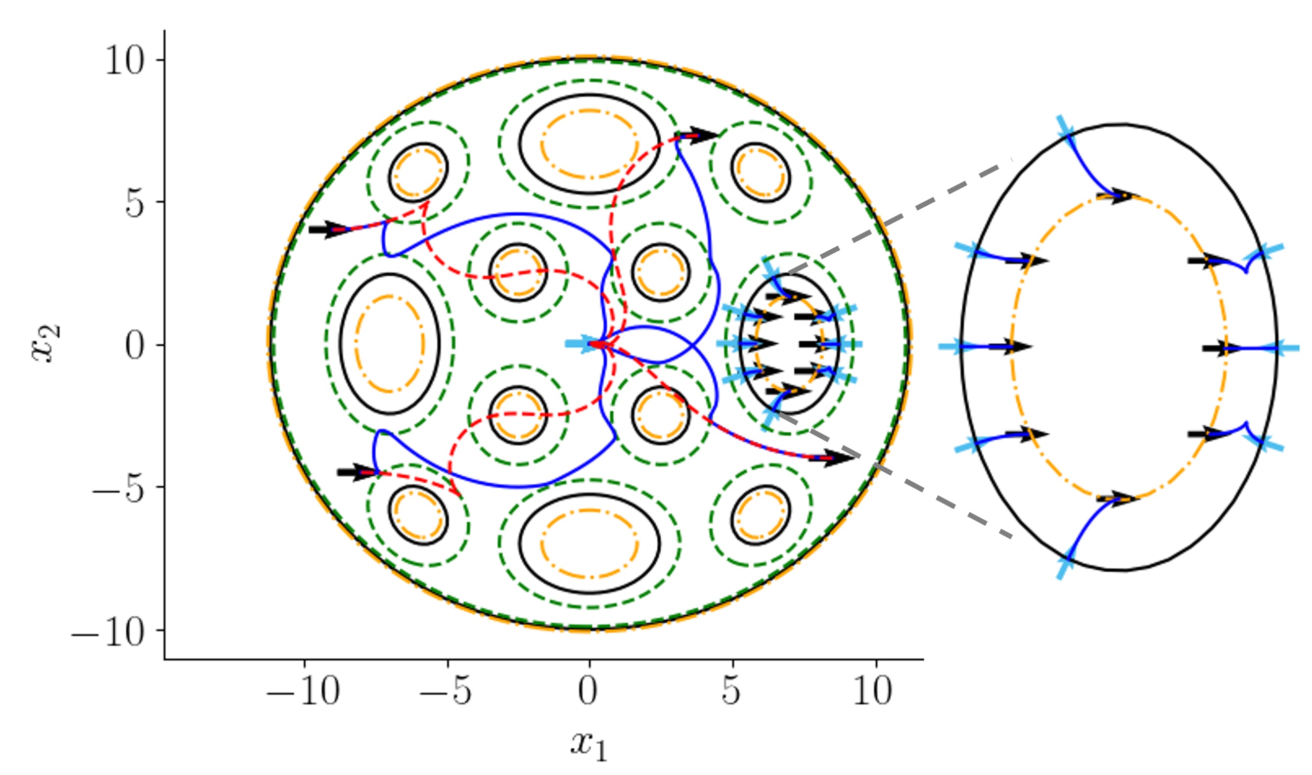
Here the goal is for a unicycle to navigate an obstacle-rich environment to reach $\bm{x}=0$ . There are 12 obstacles plus a workspace boundary yielding $N=13$ ellipsoidal constraints from (14) (see Figure 1). We define each Type-II ZCBF as (15) with $\mathscr{C}^{i}$ and $\mathscr{A}^{i}$ defined respectively by (9) and (10). The nominal controller is the stabilizing controller[23], $\bm{u}_{nom}=(u_{nom_{p}},u_{nom_{d}})$ , $u_{nom_{p}}=-k_{r}r\cos(\alpha)$ , $u_{nom_{d}}=-k_{a}\alpha-\frac{k_{r}\sin(\alpha)\cos(\alpha)(\alpha-\theta)}{\alpha}$ where $r=\sqrt{x_{1}^{2}+x_{2}^{2}}$ , $\theta=\arctan(\frac{x_{2}}{x_{1}})$ , $\alpha=x_{3}-\theta$ , and $k_{r},k_{a}\in\mathbb{R}_{>0}$ . To ensure $\bm{u}_{nom}\in\mathscr{U}$ ( $\mathscr{U}$ defined by (17)) with $\bar{u}_{p}=\bar{u}_{d}=2.0$ , $k_{r},k_{a}$ are chosen such that $k_{r}\leq\frac{\bar{u}_{p}}{r(0)}$ , $k_{a}\leq\frac{\bar{u}_{d}-k_{r}1.5\pi}{2\pi}$ . 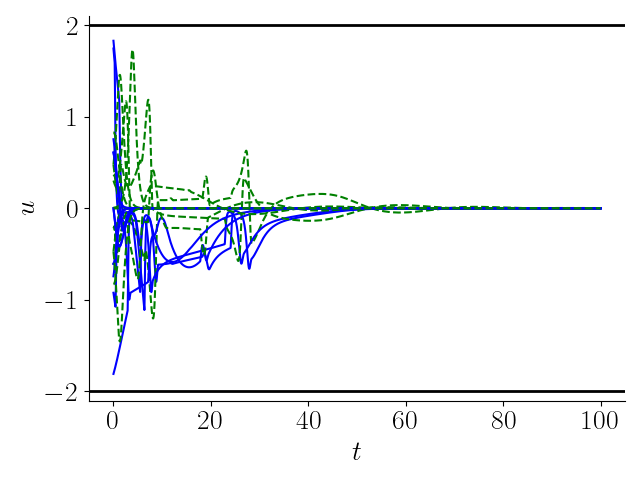For each $\mathscr{C}^{i}$ , $\bm{u}_{s_{i}}$ is defined by (16) with gains satisfying (18) such that $\bm{u}_{s_{i}}\in\mathscr{U}$ and $\kappa(h_{i})=-\frac{2}{a_{i}^{3}}h_{i}^{3}+\frac{3}{a_{i}^{2}}h_{i}^{2}$ .

Figure 1 shows the implementation of both the proposed control and the nominal control for various initial conditions. As expected, the trajectories associated with the proposed control (blue curves) avoid all obstacle regions, while converging to the origin. On the other hand, for the same initial conditions, the nominal control alone runs the unicycle through obstacle regions. To demonstrate the asymptotic stability, initial conditions were placed inside an obstacle region (zoomed part of Figure 1). For this case, we implemented the safety controller alone ( $\bm{u}_{nom}=0$ ), for which the unicycle is pushed (backwards) outside the obstacle region. Figure 2 shows the control input trajectories for the proposed control, which satisfy the desired input constraint as dictated by Theorem 3.

Refer to caption — Figure 1: Simulation results for the proposed (blue solid curves) and nominal (red dashed curves) control. $\partial\mathscr{C}^{i}$ , $\partial\mathscr{A}^{i}$ (w.r.t $h_{i}=a_{i}$ ), and $\partial\mathscr{A}^{i}$ (w.r.t $h_{i}=-b_{i}$ ) are depicted by solid black, dashed green, and dash-dotted orange curves, resp. The initial and final configurations are depicted by black and sky-blue arrows, resp.

6 Conclusion

We proposed a Type-II ZCBF for ensuring forward invariance and robustness of a constraint set, which is more general than the original ZCBF formulation. We also proposed a new control design that accommodates multiple Type-II ZCBFs with non-intersecting constraint set boundaries, while respecting input constraints. The proposed approach was applied to the classical unicycle system. Future work will address non-intersecting constraint set boundaries.

References

[1] A. D. Ames, S. Coogan, M. Egerstedt, G. Notomista, K. Sreenath, and P. Tabuada, “Control barrier functions: Theory and applications,” in European Control Conference, 2019, pp. 3420–3431.
[2] X. Xu, P. Tabuada, J. W. Grizzle, and A. D. Ames, “Robustness of control barrier functions for safety critical control,” in Proc. IFAC Conf. Anal. Design Hybrid Syst., vol. 48, 2015, pp. 54–61.
[3] W. Shaw Cortez and D. V. Dimarogonas, “Correct-by-design control barrier functions for euler-lagrange systems with input constraints,” in American Control Conference, 2020, pp. 950–955.
[4] A. D. Ames, G. Notomista, Y. Wardi, and M. Egerstedt, “Integral control barrier functions for dynamically defined control laws,” IEEE Control Systems Letters, vol. 5, no. 3, pp. 887–892, 2021.
[5] X. Xu, “Constrained control of input–output linearizable systems using control sharing barrier functions,” Automatica, vol. 87, pp. 195–201, 2018.
[6] W. Shaw Cortez, D. Oetomo, C. Manzie, and P. Choong, “Control barrier functions for mechanical systems: Theory and application to robotic grasping,” IEEE Trans. Control Syst. Technol., vol. 29, no. 2, pp. 530–545.
[7] J. Breeden, K. Garg, and D. Panagou, “Control barrier functions in sampled-data systems,” IEEE Control Systems Letters, vol. 6, pp. 367–372, 2022.
[8] G. Yang, C. Belta, and R. Tron, “Self-triggered control for safety critical systems using control barrier functions,” in American Control Conference, 2019, pp. 4454–4459.
[9] M. Jankovic, “Robust control barrier functions for constrained stabilization of nonlinear systems,” Automatica, vol. 96, pp. 359–367, 2018.
[10] A. Alan, A. J. Taylor, C. R. He, G. Orosz, and A. D. Ames, “Safe controller synthesis with tunable input-to-state safe control barrier functions,” IEEE Control Systems Letters, vol. 6, pp. 908–913, 2021.
[11] B. T. Lopez, J.-J. E. Slotine, and J. P. How, “Robust adaptive control barrier functions: An adaptive and data-driven approach to safety,” IEEE Control Systems Letters, vol. 5, no. 3, pp. 1031–1036, 2021.
[12] X. Tan, W. Shaw Cortez, and D. V. Dimarogonas, “High-order barrier functions: Robustness, safety and performance-critical control,” IEEE Transactions on Automatic Control, 2021, early access.
[13] W. Xiao and C. Belta, “Control barrier functions for systems with high relative degree,” in IEEE Conference on Decision and Control, 2019, pp. 27–34.
[14] A. D. Ames, X. Xu, J. W. Grizzle, and P. Tabuada, “Control barrier function based quadratic programs for safety critical systems,” IEEE Transactions on Automatic Control, vol. 62, no. 8, pp. 3861–3876, 2017.
[15] W. Shaw Cortez and D. V. Dimarogonas, “Safe-by-design control for Euler-Lagrange systems,” 2021. [Online]. Available: https://arxiv.org/abs/2009.03767
[16] H. Brezis, “On a characterization of flow-invariant sets,” Communications on Pure and Applied Mathematics, vol. 23, no. 2, pp. 261–263, 1970.
[17] H. K. Khalil, Nonlinear Systems. Upper Saddle River, N.J. : Prentice Hall, c2002., 2002.
[18] M. I. El-Hawwary and M. Maggiore, “Passivity-based stabilization of non-compact sets,” in IEEE on Decision and Control, 2007, pp. 1734–1739.
[19] N. P. Bathia and G. P. Szegö, Dynamical Systems: Stability Theory and Applications. Springer-Verlag Berlin.
[20] M. I. El-Hawwary and M. Maggiore, “Stabilization of closed sets for passive systems, part II: passivity-based control,” in IEEE Conference on Decision and Control, 2008, pp. 3799–3804.
[21] W. Shaw Cortez, C. Verginis, and D. V. Dimarogonas, “Safe, passive control for mechanical systems with application to physical human-robot interactions,” in IEEE International Conference on Robotics and Automation, 2021.
[22] W. W. Hager, “Lipschitz continuity for constrained processes,” SIAM Journal on Control and Optimization, vol. 17, no. 3, pp. 321–338, 1979.
[23] M. Aicardi, G. Casalino, A. Bicchi, and A. Balestrino, “Closed loop steering of unicycle like vehicles via Lyapunov techniques,” IEEE Robotics Automation Magazine, vol. 2, no. 1, pp. 27–35, 1995.