A Runtime-Based Computational Performance Predictor for
Deep Neural Network Training

Geoffrey X. Yu
University of Toronto
Vector Institute Yubo Gao
University of Toronto Pavel Golikov
University of Toronto
Vector Institute Gennady Pekhimenko
University of Toronto
Vector Institute

Abstract

Deep learning researchers and practitioners usually leverage GPUs to help train their deep neural networks (DNNs) faster. However, choosing which GPU to use is challenging both because (i) there are many options, and (ii) users grapple with competing concerns: maximizing compute performance while minimizing costs. In this work, we present a new practical technique to help users make informed and cost-efficient GPU selections: make performance predictions with the help of a GPU that the user already has. Our technique exploits the observation that, because DNN training consists of repetitive compute steps, predicting the execution time of a single iteration is usually enough to characterize the performance of an entire training process. We make predictions by scaling the execution time of each operation in a training iteration from one GPU to another using either (i) wave scaling, a technique based on a GPU’s execution model, or (ii) pre-trained multilayer perceptrons. We implement our technique into a Python library called Habitat and find that it makes accurate iteration execution time predictions (with an average error of 11.8%) on ResNet-50, Inception v3, the Transformer, GNMT, and DCGAN across six different GPU architectures. Habitat supports PyTorch, is easy to use, and is open source.¹¹1Habitat is available on GitHub: github.com/geoffxy/habitat [105, 106]

1 Introduction

Over the past decade, deep neural networks (DNNs) have seen incredible success across many machine learning tasks [37, 93, 50, 39, 96, 99, 26]—leading them to become widely used throughout academia and industry. However, despite their popularity, DNNs are not always straightforward to use in practice because they can be extremely computationally-expensive to train [53, 109, 23, 95]. This is why, over the past few years, there has been a significant and ongoing effort to bring hardware acceleration to DNN training [80, 78, 45, 16, 35, 36, 10].

As a result of this effort, today there is a vast array of hardware options for deep learning users to choose from for training. These options range from desktop and server-class GPUs (e.g., 2080Ti [70] and A100 [78]) all the way to specialized accelerators such as the TPU [45], AWS Trainium [10], Gaudi [36], IPU [35], and Cerebras WSE [16]. Having all these options offers flexibility to users, but at the same time can also lead to a paradox of choice: which hardware option should a researcher or practitioner use to train their DNNs?

A natural way to start answering this question is to first consider CUDA-enabled GPUs. This is because they (i) are commonly used in deep learning; (ii) are supported by all major deep learning software frameworks (PyTorch [86], TensorFlow [1], and MXNet [19]); (iii) have mature tooling support (e.g., CUPTI [76]); and (iv) are readily available for rent and purchase. In particular, when considering GPUs, we find that that there are many situations where a deep learning user needs to choose a specific GPU to use for training:

•

Choosing between different hardware tiers. In both academia and industry, deep learning users often have access to several tiers of hardware: (i) a workstation with a GPU used for development (e.g., 2080Ti), (ii) a private GPU cluster that is shared within their organization (e.g., RTX6000 [84]), and (iii) GPUs that they can rent in the cloud (e.g., V100 [66]). Each tier offers a different cost, availability, and performance trade-off. For example, a private cluster might be “free” (in monetary cost) to use, but jobs may be queued because the cluster is also shared among other users. In contrast, cloud GPUs can be rented on-demand for exclusive use.
•

Deciding on which GPU to rent or purchase. Cloud providers make many different GPUs available for rent (e.g., P100 [62], V100, T4 [71], and A100 [78]), each with different performance at different prices. Similarly, a wide variety of GPUs are available for purchase (e.g., 2080Ti, 3090 [82]) both individually and as a part of pre-built workstations [52]. These GPUs can vary up to $6\times$ in price [98] and $6\times$ in peak performance [79].
•

Determining how to schedule a job in a heterogeneous GPU cluster. A compute cluster (e.g., operated by a cloud provider [8, 32, 58]) may have multiple types of GPUs available that can handle a training workload. Deciding which GPU to use for a job will typically depend on the job’s priority and performance on the GPU being considered [61, 18].
•

Selecting alternative GPUs. When a desired GPU is unavailable (e.g., due to capacity constraints in the cloud), a user may want to select a different GPU with a comparable cost-normalized performance. For example, when training ResNet-50 [37] on Google Cloud [31], we find that both the P100 and V100 have similar cost-normalized throughputs (differing by just 0.8%). If the V100 were to be unavailable,²²2In our experience, we often ran into situations where the V100 was unavailable for rent because the cloud provider had an insufficient supply. a user may decide to use the P100 instead since the total training cost would be similar.

What makes these situations interesting is that there is not necessarily a single “correct” choice. Users make GPU selections based on whether the performance benefits of the chosen configuration are worth the cost to train their DNNs. But making these selections in an informed way is not easy, as performance depends on many factors simultaneously: (i) the DNN being considered, (ii) the GPU being used, and (iii) the underlying software libraries used during training (e.g., cuDNN [74], cuBLAS [77]).

To do this performance analysis today, the common wisdom is to either (i) directly measure the computational performance (e.g., throughput) by actually running the training job on the GPU, or (ii) consult existing benchmarks (e.g., MLPerf [53]) published by the community to get a “ballpark estimate.” While convenient, these approaches also have their own limitations. Making measurements requires users to already have access to the GPUs they are considering; this may not be the case if a user is deciding whether or not to buy or rent that GPU in the first place. Secondly, benchmarks are usually only available for a subset of GPUs (e.g., the V100 and T4) and only for common “benchmark” models (e.g., ResNet-50 [37] and the Transformer [99]). They are not as helpful if you need an accurate estimate of the performance of a custom DNN on a specific GPU (a common scenario when doing deep learning research).

In this work, we make the case for a third complementary approach: making performance predictions. Although predicting the performance of general compute workloads can be prohibitively difficult due to the large number of possible program phases, we observe that DNN training workloads are special because they contain repetitive computation. DNN training consists of repetitions of the same (relatively short) training iteration, which means that the performance of an entire training process can be characterized by just a few training iterations.

⬇

import habitat

\partracker = habitat.OperationTracker(

origin_device=habitat.Device.RTX2070,

)

\parwith tracker.track():

run_my_training_iteration()

\partrace = tracker.get_tracked_trace()

print("Pred. iter. exec. time: {:.2f} ms".format(

trace.to_device(habitat.Device.V100).run_time_ms,

))

Figure 1: An example of how Habitat can be used to make iteration execution time predictions.

We leverage this observation to build a new technique that predicts a DNN’s training iteration execution time for a given batch size and GPU using both runtime information and hardware characteristics. We make predictions in two steps: (i) we measure the execution time of a training iteration on an existing GPU, and then (ii) we scale the measured execution times of each individual operation onto a different GPU using either wave scaling or pre-trained multilayer perceptrons (MLPs) [29]. Wave scaling is a technique that applies scaling factors to the GPU kernels in an operation, based on a mix of the ratios between the two GPUs’ memory bandwidth and compute units. We use MLPs for certain operations (e.g., convolution) where the kernels used differ between the two GPUs; we describe this phenomenon and the MLPs in more detail in Sections 3.2 and 3.4. We believe that using an existing GPU to make operation execution time predictions for a different GPU is reasonable because deep learning users often already have a local GPU that they use for development.

We implement our technique into a Python library that we call Habitat, and evaluate its prediction accuracy on five DNNs that have applications in image classification, machine translation, and image generation: (i) ResNet-50, (ii) Inception v3 [97] (iii) the Transformer, (iv) GNMT [102], and (v) DCGAN [89]. We use Habitat to make iteration execution time predictions across six different GPUs and find that it makes accurate predictions with an average error of 11.8%. Additionally, we present two case studies to show how Habitat can be used to help users make accurate cost-efficient GPU selections according to their needs (Section 5.3).

We designed Habitat to be easy and practical to use (see Listing 1). Habitat currently supports PyTorch [86] and is open source: github.com/geoffxy/habitat [105, 106].

In summary, this work makes the following contributions:

•

Wave scaling: a new technique that scales the execution time of a kernel measured on one GPU to a different GPU by using scaled ratios between the (i) number of compute units on each GPU, and (ii) their memory bandwidths.
•

The implementation and evaluation of Habitat: a new library that uses wave scaling along with pre-trained MLPs to predict the execution time of DNN training iterations on different GPUs.

2 Why Predict the Computational Training Performance of DNNs on Different GPUs?

This work presents a new practical technique for predicting the execution time of a DNN training iteration on different GPUs, with the goal of helping deep learning users make informed cost-efficient GPU selections. However, a common first question is to ask why we need to make these performance predictions in the first place. Could other performance comparison approaches (e.g., simple heuristics or measurements) be used instead? In this section, after providing some background about DNN training, we outline the problems with these alternative approaches to further motivate the need for practical performance predictions.

2.1 Background on DNN Training

DNNs, at their heart, are mathematical functions that produce predictions given an input and a set of learned parameters, also known as weights [29]. They are built by combining together a series of different layers, each of which may contain weights. The layers map to mathematical operations. For example, a fully connected layer is implemented using matrix multiplication [29]. To produce predictions, a DNN takes a tensor (an $n$ -dimensional array) as input and applies the operations associated with each layer in sequence.

Training.

A DNN learns its weights in an iterative process called training. Each training iteration operates on a batch of labelled inputs and consists of a forward pass, backward pass (using backpropagation [90]), and weight update. The forward and backward passes compute gradients for the weights, which are then used by an optimization algorithm (e.g., stochastic gradient descent [12] or Adam [49]) to update the weights so that the DNN produces better predictions. These steps are repeated until the DNN makes acceptably accurate predictions.

Computational performance.

Although conceptually simple, prior work has shown that DNN training can be an extremely time-consuming process [53, 23, 109, 95]. There are two primary factors that influence the time it takes a DNN to reach an acceptable accuracy during training [59]: (i) statistical efficiency, and (ii) hardware efficiency. Statistical efficiency governs the number of training iterations (i.e., weight updates) required to reach a target test accuracy whereas hardware efficiency governs how quickly a training iteration runs. In this work, we focus on helping deep learning users make informed cost-efficient hardware configuration selections to improve their DNN’s hardware efficiency. As a result, we compare the performance of different GPUs when training a DNN using the time it takes a training iteration to run. This metric equivalently captures the training throughput for that particular DNN.

2.2 Why Not Measure Performance Directly?

Perhaps the most straightforward approach to compare the performance of different GPUs is to just measure the iteration execution time (and hence, throughput) on each GPU when training a given DNN. However, this approach also has a straightforward downside: it requires the user to actually have access to the GPU(s) being considered in the first place. If a user is looking to buy or rent a cost-efficient GPU, they would ideally want to know its performance on their DNNs before spending money to get access to the GPU.

Refer to caption — Figure 2: DCGAN iteration execution time predictions, and their errors, made from the T4 using peak FLOPS ratios between the devices. Using simple heuristics can lead to high prediction errors.

2.3 Why Not Apply Heuristics?

Another approach is to use heuristics based on the hardware specifications published by the manufacturer. For example, one could use the ratio between the peak floating point operations per second (FLOPS) of two GPUs or the ratio between the number of CUDA cores on each GPU. The problem with this approach is that these heuristics do not always work. Heuristics often assume that a DNN training workload can exhaust all the computational resources on a GPU, which is not true in general [109].

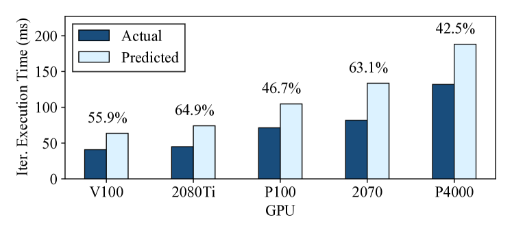
To show an example of when simple heuristics do not work well, we use a GPU’s peak FLOPS to make iteration execution time predictions. We measure the execution time of a DCGAN training iteration on the T4³³3We use a batch size of 128 LSUN [104] synthetic inputs. See Section 5.1 for details about our methodology. and then use this measurement to predict the iteration execution time on different GPUs by multiplying by the ratio between the devices’ peak FLOPS. Figure 2 shows the measured and predicted execution times on each GPU, along with the prediction error as a percentage. The main takeaway from this figure is that using simple heuristics can lead to high prediction errors; the highest prediction error in this experiment is 64.9%, and all the prediction errors are at least 42.5%. In contrast, Habitat can make these exact same predictions with an average error of 10.2% (maximum 21.8%).

2.4 Why Not Use Benchmarks?

A third potential approach is to consult published benchmarking results [53, 109, 23, 81]. However, the problem with relying on benchmarking results is that they are limited to a set of “common” DNNs (e.g., ResNet-50 or BERT [26]) and are usually only available for a small selection of GPUs (e.g., the T4, V100, and A100). Moreover, benchmarking results also vary widely among different models and GPUs [53, 109, 81]. Therefore if no results exist for the GPU(s) a user is considering, or if a user is working with a new DNN architecture, there will be no benchmark results for them to consult.

2.5 Why Not Always Use the “Best” GPU?

Finally, a fourth approach is to always use the most “powerful” GPU available with the assumption that GPUs are already priced based on their performance. Why make performance predictions when the cost-efficiency of popular GPUs should be the same? However, this assumption is a misconception. Prior work has already shown examples where the performance benefits of different GPUs changes depending on the model [61, 18, 109]. In this work, we also show additional examples in our case studies (Section 5.3) where (i) cost-efficiency leads to selecting a different GPU, and (ii) where the V100 does not offer significant performance benefits over a common desktop-class GPU (the 2080Ti).

Summary.

Straightforward approaches that users might consider to make GPU selections all have their own downsides. In particular, existing approaches either require access to the GPUs themselves or are only applicable for common DNNs and GPUs. Therefore there is a need for a complementary approach: making performance predictions—something that we explore in this work.

3 Habitat

Our approach to performance predictions is powered by three key observations. In this section, after describing these observations, we outline the key ideas behind Habitat.

3.1 Key Observations

Observation 1: Repetitive computation.

While training a DNN to an acceptable accuracy can take on the order of hours to days [53, 23, 109], a single training iteration takes on the order of hundreds of milliseconds. This observation improves the predictability of DNN training as we can characterize the performance of an entire DNN training session using the performance of a single iteration.

Observation 2: Common building blocks among DNNs.

Although DNNs can consist of hundreds of operations, they are built using a relatively small set of unique operations. For example, convolutional neural networks typically comprise convolutional, pooling, fully connected, and batch normalization [42] layers. This observation reduces the problem of predicting the performance of an arbitrary DNN’s training iteration to developing prediction mechanisms for a small set of operations.

Observation 3: Runtime information available.

When developing DNNs, users often have a GPU available for use in their workstations. These GPUs are used for development purposes and are not necessarily chosen for the highest performance (e.g., 1080Ti [64], TITAN Xp [68]). However, they can be used to provide valuable runtime information about the GPU kernels that are used to implement a given DNN. In Section 3.3, we describe how we can leverage this runtime information to predict the performance of the GPU kernels on different GPUs (e.g., from a desktop-class GPU such as the 2080Ti [70] to a server-class GPU such as the V100 [66, 67]).

3.2 Habitat Overview

Habitat records information at runtime about a DNN training iteration for a specific batch size on a given GPU (Observation 3) and then uses that information to predict the training iteration execution time on a different GPU (for the same batch size). Predicting the iteration execution time is enough (Observation 1) to compute metrics about the entire training process on different GPUs. These predicted metrics, such as the training throughput and cost-normalized throughput, are then used by end-users (e.g., deep learning researchers) to make informed hardware selections.

To actually make these predictions for a different GPU, Habitat predicts the new execution time of each individual operation in a training iteration. Habitat then adds these predicted times together to arrive at an execution time prediction for the entire iteration. For an individual operation, Habitat makes predictions using either (i) wave scaling (Section 3.3), or (ii) pre-trained MLPs (Section 3.4).

The reason why Habitat uses two techniques together is that wave scaling assumes that the same GPU kernels are used to implement a given DNN operation on each GPU. However, some DNN operations are implemented using different GPU kernels on different GPUs (e.g., convolutions, recurrent layers). This is done for performance reasons as these operations are typically implemented using proprietary kernel libraries that leverage GPU architecture-specific kernels (e.g., cuDNN [21], cuBLAS [77]). We refer to these operations as kernel-varying, and scale their execution times to different GPUs using pre-trained MLPs. Habitat uses wave scaling for the rest of the operations, which we call kernel-alike.

3.3 Wave Scaling

Wave scaling works by scaling the execution times of the kernels used to implement a kernel-alike DNN operation. The computation performed by a GPU kernel is partitioned into groups of threads called thread blocks [28], which typically execute in concurrent groups, resulting in waves of execution. The key idea behind wave scaling is to compute the number of thread block waves in a kernel and scale the wave execution time using ratios between the origin and destination GPUs.

We describe wave scaling formally in Equation 1. Let $T_{i}$ represent the execution time of the kernel on GPU $i$ , $B$ the number of thread blocks in the kernel, $W_{i}$ the number of thread blocks in a wave on GPU $i$ , $D_{i}$ the memory bandwidth on GPU $i$ , and $C_{i}$ the clock frequency on GPU $i$ . Here we let $i\in\{o,d\}$ to represent the origin and destination GPUs. By measuring $T_{o}$ (Observation 3), wave scaling predicts $T_{d}$ using

T_{d}=\left\lceil{\frac{B}{W_{d}}}\right\rceil\left(\frac{D_{o}}{D_{d}}\frac{W_{d}}{W_{o}}\right)^{\gamma}\left(\frac{C_{o}}{C_{d}}\right)^{1-\gamma}\left\lceil{\frac{B}{W_{o}}}\right\rceil^{-1}T_{o}

(1)

where $\gamma\in[0,1]$ represents the “memory bandwidth boundedness” of the kernel. Habitat selects $\gamma$ by measuring the kernel’s arithmetic intensity and then leveraging the roofline model [101] (see Section 4.2).

As shown in Equation 1, wave scaling uses the ratios between the GPUs’ (i) memory bandwidths, (ii) clock frequencies, and (iii) the size of a wave on each GPU. The intuition behind factors (i) and (iii) is that a higher relative memory bandwidth allows more memory requests to be served in parallel whereas having more thread blocks in a wave results in more memory requests being made. Thus, everything else held constant, waves in memory bandwidth bound kernels (i.e., large $\gamma$ ) should see speedups on GPUs with more memory bandwidth. The intuition behind factor (ii) is that higher clock frequencies may benefit waves in compute bound kernels (i.e., small $\gamma$ ).⁴⁴4The clock’s impact on execution time depends on other factors too (e.g., the GPU’s instruction set architecture). Wave scaling aims to be a simple and understandable model and therefore does not model these complex effects.

For large $\left\lceil{B/W_{i}}\right\rceil$ (i.e., when there are a large number of waves) we get that $\left\lceil{B/W_{i}}\right\rceil\approx B/W_{i}$ . In this case, Equation 1 simplifies to

T_{d}=\left(\frac{D_{o}}{D_{d}}\right)^{\gamma}\left(\frac{W_{o}}{W_{d}}\right)^{1-\gamma}\left(\frac{C_{o}}{C_{d}}\right)^{1-\gamma}T_{o}

(2)

Habitat uses Equation 2 to predict kernel execution times because we find that in practice, most kernels are composed of many thread blocks.

Habitat computes $W_{i}$ for each kernel and GPU using the thread block occupancy calculator that is provided as part of the CUDA Toolkit [80]. We obtain $C_{i}$ from each GPU’s specifications, and we obtain $D_{i}$ by measuring the achieved bandwidth on each GPU ahead of time. Note that we make these measurements once and then distribute them in a configuration file with Habitat.

3.4 MLP Predictors

To handle kernel-varying operations, Habitat uses pre-trained MLPs to make execution time predictions. We treat this prediction task as a regression problem: given a series of input features about the operation and a target GPU (described below), predict the operation’s execution time on that target GPU. We learn an MLP for each kernel-varying operation that Habitat currently supports: (i) convolutions (2-dimensional), (ii) LSTMs [38], (iii) batched matrix multiplies, and (iv) linear layers (matrix multiply with an optional bias term). As we show in Section 5, relatively few DNN operations are kernel-varying⁵⁵5This is, in part, because implementing performant architecture-specific kernels for each kernel-varying operation takes significant engineering effort. and so training separate MLPs for each of these operations is a feasible approach. Furthermore, these MLPs can be used for many different DNNs as these operations are common “building blocks” used in DNNs (Observation 2).

Input features.

Each operation-specific MLP takes as input: (i) layer dimensions (e.g., the number of input and output channels in a convolution); (ii) the memory capacity and bandwidth on the target GPU; (iii) the number of streaming multiprocessors (SMs) on the target GPU; and (iv) the peak FLOPS of the target GPU, specified by the manufacturer.

Model architecture.

Each MLP comprises an input layer, eight hidden layers, and an output layer that produces a single real number—the predicted execution time (this includes the forward and backward pass) for the MLP’s associated operation. We use ReLU activation functions in each layer and we use 1024 units in each hidden layer. We outline the details behind our datasets and how these MLPs are trained in Section 4.3.

4 Implementation Details

Habitat is built to work with PyTorch [86]. However, the ideas behind Habitat are general and straightforward to implement in other frameworks as well. Habitat performs its analysis using a DNN’s computation graph, which is also available in other frameworks (e.g., TensorFlow [1] and MXNet [19]).

4.1 Extracting Runtime Metadata

Habitat extracts runtime metadata in a training iteration by “monkey patching” PyTorch operations with special wrappers. These wrappers allow Habitat to intercept and keep track of all the operations that run in one training iteration, as they are executed. As shown in Listing 1, users explicitly indicate to Habitat when to start and stop tracking the operations in a DNN by calling track().

Execution time.

To measure the execution time of each operation, Habitat re-runs each operation independently with the same inputs as recorded when the operation was intercepted. Habitat also measures the execution time associated with the operation’s backward pass, if applicable. The reason why Habitat makes measurements by re-running the individual operations is that the operations could be very short (in execution time). Thus, Habitat needs to run them multiple times to make accurate measurements. Habitat uses CUDA events [73] to make these timing measurements.

Kernel metadata and metrics.

Habitat uses CUPTI [76] to record execution times and metrics (see Section 4.2) for the kernels used to implement each operation in the DNN. This information is used by wave scaling.

4.2 Selecting Gamma ( $\gamma$ )

Recall from Section 3.3 that wave scaling scales its ratios using $\gamma$ , a factor that represents the “memory bandwidth boundedness” of a kernel. In this section, we describe in more detail how Habitat automatically selects $\gamma$ for each kernel.

Roofline model.

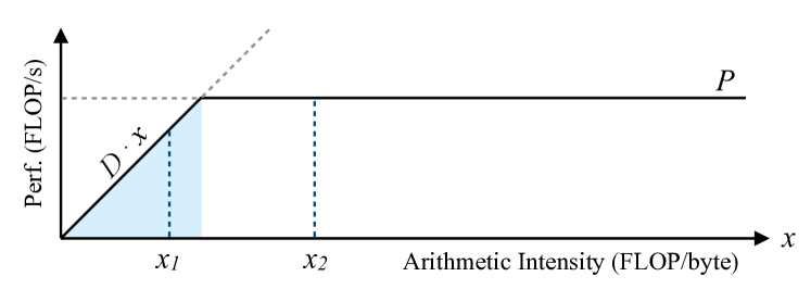
Habitat uses the roofline model [101] to estimate a kernel’s memory boundedness. Figure 3 shows an example roofline model. The roofline model introduces the notion of a kernel’s arithmetic intensity: the number of floating point operations it performs per byte of data read or written to memory (represented by $x$ in Figure 3).

A key idea behind the roofline model is that it models a kernel’s peak performance as the minimum of either the hardware’s peak performance ( $P$ ) or the hardware’s memory bandwidth times the kernel’s arithmetic intensity ( $D\cdot x$ ) [101]. This minimum is shown by the solid line in Figure 3. The arithmetic intensity where these two limits meet is called the “ridge point” ( $R$ ), where $R=P/D$ . The model considers a kernel with an arithmetic intensity of $x$ to be memory bandwidth bound if $x<R$ and compute bound otherwise. For example, in Figure 3, a kernel with an arithmetic intensity of $x_{1}$ would be considered memory bandwidth bound whereas a kernel with an intensity of $x_{2}$ would be considered compute bound.

Wave scaling leverages the observation that a kernel’s arithmetic intensity is fixed across GPUs (i.e., arithmetic intensity only depends on the kernel’s code). $R$ changes across GPUs because $P$ and $D$ vary among GPUs, but can be computed using a GPU’s performance specifications. Therefore, if Habitat computes a kernel’s arithmetic intensity, it can use the arithmetic intensity’s distance from the destination GPU’s ridge point to estimate the kernel’s memory bandwidth boundedness (on the destination GPU).

Selecting $\gamma$ .

When profiling each kernel, Habitat gathers metrics that allow it to empirically calculate the kernel’s arithmetic intensity (floating point efficiency, number of bytes read and written to DRAM). If we let $x$ be the kernel’s measured arithmetic intensity and $R=P/D$ for the destination GPU (using the notation presented above), Habitat sets $\gamma$ using

\gamma=\begin{cases}(-0.5/R)x+1&\mathrm{if\ }x<R\\ 0.5R/x&\mathrm{otherwise}\end{cases}

(3)

This equation means that $\gamma$ decreases linearly from 1 to 0.5 as $x$ increases toward $R$ . After passing $R$ , $\gamma$ approaches 0 as $x$ approaches infinity.

Practical optimizations.

In practice, gathering metrics on GPUs is a slow process because the kernels need to be replayed multiple times to capture all the needed performance counters. To address this challenge, we make two optimizations: (i) we cache measured metrics, keyed by the kernel’s name and its launch configuration (number of thread blocks and block size); and (ii) we only measure metrics for operations that contribute significantly to the training iteration’s execution time (e.g., with execution times at or above the 99.5th percentile). Consequently, when metrics are unavailable for a particular kernel, we set $\gamma=1$ . We believe that this is a reasonable approximation because kernel-alike operations tend to be very simple (e.g., element-wise operations) and are therefore usually memory bandwidth bound.

4.3 MLPs: Data and Training

In this section, we describe the details behind Habitat’s MLPs: how we (i) collect training data, (ii) preprocess the data, and (iii) train the MLPs.

4.3.1 Data Collection

We gather training data by measuring the forward and backward pass execution times of kernel-varying operations at randomly sampled input configurations. An input configuration is a setting of an operation’s parameters (e.g., batch size and number of channels in a convolution). We use predefined ranges for each operation’s parameters, as described in more detail below, and ignore any configurations that result in running out of memory. We make these measurements for all six of the GPUs listed in Section 5.1. We use the same seed when sampling on different GPUs to ensure we have measurements for the same random input configurations across all the GPUs. We create the final dataset by joining data entries that have the same operation and configuration, but with different GPUs.

2D convolutions.

For convolutions, we vary the (i) batch size (1 – 64), (ii) number of input (3 – 2048) and output channels (16 – 2048), (iii) kernel size (1 – 11), (iv) padding (0 – 3), (v) stride (1 – 4), (vi) image size (1 – 256), and (vii) whether or not there is a bias weight. We only sample configurations with square images and kernel sizes. During sampling, we ignore any configurations that result in invalid arguments (e.g., a kernel size larger than the image). We selected these parameter ranges by surveying the convolutional neural networks included in PyTorch’s torchvision package [24].

LSTMs.

For LSTMs, we vary the (i) batch size (1 – 128), (ii) number of input features (1 – 1280), (iii) number of hidden features (1 – 1280), (iv) sequence length (1 – 64), (v) number of stacked layers (1 – 6), (vi) whether or not the LSTM is bidirectional, and (vii) whether or not there is a bias weight.

Batched matrix multiply (bmm).

For a batched matrix multiply of $A\times B$ where $A\in\mathbb{R}^{n\times l\times m}$ and $B\in\mathbb{R}^{n\times m\times r}$ , we vary the (i) batch size ( $n$ ) (1 – 128), and (ii) the $l$ , $m$ , and $r$ dimensions (1 – 1024).

Linear layers.

For linear layers, we vary the (i) batch size (1 – 3500), (ii) input features (1 – 32768), (iii) output features (1 – 32768), and (iv) whether or not there is a bias weight.

4.3.2 Data Preprocessing

After collecting data on the GPUs, we build one dataset per operation by (i) adding the forward and backward execution times to arrive at a single execution time for each operation instance on a particular GPU, and (ii) attaching additional GPU hardware features to each of these data points. We attach the GPU’s (i) memory capacity and bandwidth; (ii) number of streaming multiprocessors (SMs); and (iii) peak FLOPS, as specified by the GPU manufacturer.

We present the characteristics of the final datasets in Table 1. We add four to the number of features to account for the four GPU features (described above) that we add to each data point. Similarly, in the dataset size column we show the total number of unique operation configurations that we sample. We multiply by six because we make measurements on six different GPUs.

Table 1: A summary of the datasets used for our MLPs.

Operation	Features	Dataset Size
2D Convolution	$7+4$	$91,138\times 6$
LSTM	$7+4$	$124,176\times 6$
Batched Matrix Multiply	$4+4$	$131,022\times 6$
Linear Layer	$4+4$	$155,596\times 6$

4.3.3 Training

We implement our MLPs using PyTorch. We train each MLP for 80 epochs using the Adam optimizer [49] with a learning rate of $5\times 10^{-4}$ , weight decay of $10^{-4}$ , and a batch size of 512 samples. We reduce the learning rate to $10^{-4}$ after 40 epochs. We use the mean absolute percentage error as our loss function:

L=\frac{1}{n}\sum_{i=1}^{n}\left|\frac{\mathrm{predicted}_{i}-\mathrm{measured}_{i}}{\mathrm{measured}_{i}}\right|

We assign 80% of our data samples to the training set and the rest to our test set. None of the configurations that we test on in Section 5 appear in our training sets. We normalize the inputs by subtracting by the mean and dividing by the standard deviation of the input features in our training set.

5 Evaluation

Habitat is meant to be used by deep learning researchers and practitioners to predict the potential compute performance of a given GPU so that they can make informed cost-efficient choices when selecting GPUs for training. Consequently, in our evaluation our goals are to determine (i) how accurately Habitat can predict the training iteration execution time on GPUs with different architectures, and (ii) whether Habitat can correctly predict the relative cost-efficiency of different GPUs when used to train a given model. Overall, we find that Habitat makes iteration execution time predictions across pairs of six different GPUs with an average error of 11.8% on ResNet-50 [37], Inception v3 [97], the Transformer [99], GNMT [102], and DCGAN [89].

5.1 Methodology

Table 2: The GPUs we use in our evaluation.

GPU	Generation	Mem.	Mem. Type	SMs	Rental Cost⁶⁶6Google Cloud pricing in us-central1, as of June 2021.
P4000 [65]	Pascal [63]	8 GB	GDDR5 [56]	14	–
P100 [62]	Pascal [63]	16 GB	HBM2 [4]	56	$1.46/hr
V100 [66]	Volta [67]	16 GB	HBM2	80	$2.48/hr
2070 [69]	Turing [72]	8 GB	GDDR6 [57]	36	–
2080Ti [70]		11 GB	GDDR6	68	–
T4 [71]		16 GB	GDDR6	40	$0.35/hr

Table 3: The machines we use in our evaluation.

CPU	Freq.	Cores	Main Mem.	GPU
Xeon E5-2680 v4 [41]	2.4 GHz	14	128 GB	P4000
Ryzen TR 1950X [5]	3.4 GHz	16	16 GB	2070
EPYC 7371 [6]	3.1 GHz	16	128 GB	2080Ti

Table 4: The DNNs and training configurations we use.

Application	Model	Arch. Type	Dataset
Image Classif.	ResNet-50 [37]	Convolution	ImageNet [91]
	Inception v3 [97]
Machine Transl.	GNMT [102]	Recurrent	WMT’16 [11] (EN-DE)
	Transformer [99]	Attention	WMT’16 [11] (EN-DE)
Image Gen.	DCGAN [89]	Convolution	LSUN [104]

Hardware.

In our experiments, we use the GPUs listed in Table 2. For the P4000, 2070, and 2080Ti we use machines whose configurations are listed in Table 3. For the T4 and V100, we use g4dn.xlarge and p3.2xlarge instances on AWS respectively [7]. For the P100, we use Google Cloud’s n1-standard instances [30] with 4 vCPUs and 15 GB of system memory.

Runtime environment.

We run our experiments inside Docker containers [27]. Our container image uses Ubuntu 18.04 [15], CUDA 10.1 [80], and cuDNN 7 [74]. On cloud instances, we use the NVIDIA GPU Cloud Image, version 20.06.3 [83]. We use PyTorch 1.4.0 [86] for all experiments.

Models and datasets.

We evaluate Habitat by predicting the training iteration execution time for the models listed in Table 4 on different GPUs. For ResNet-50 and Inception v3 we use stochastic gradient descent [12]. We use Adam [49] for the rest of the models. We use synthetic data (sampled from a normal distribution) of the same size as samples from each dataset.⁷⁷7We verified that the training computation time does not depend on the values of the data itself. For the machine translation models, we use a fixed sequence length of 50—the longest sentence length typically used—to show how Habitat can make predictions for a lower bound on the computational performance.

Metrics.

In our experiments, we measure and predict the training iteration execution time—the wall clock time it takes to perform one training step on a batch of inputs. We use the training iteration execution time to compute the training throughput and cost-normalized throughput for our analysis. The training throughput is the batch size divided by the iteration execution time. The cost-normalized throughput is the throughput divided by the hourly cost of renting the hardware.

Measurements.

We use CUDA events to measure the execution time of training iterations and DNN operations. We run 3 warm up repetitions, which we discard, and then record the average execution time over 3 further repetitions. We use CUPTI [76] to measure a kernel’s execution time.

5.2 How Accurate are Habitat’s Predictions?

To evaluate Habitat’s prediction accuracy, we use it to make training iteration execution time predictions for ResNet-50, Inception v3, the Transformer, GNMT, and DCGAN on all six GPUs listed in Section 5.1. Recall that Habitat makes execution time predictions by scaling the execution time of a model and specific batch size measured on one GPU (the “origin” GPU) to another (the “destination” GPU). As a result, we use all 30 possible (origin, destination) pairs of these six GPUs in our evaluation.

5.2.1 End-to-End Prediction Accuracy

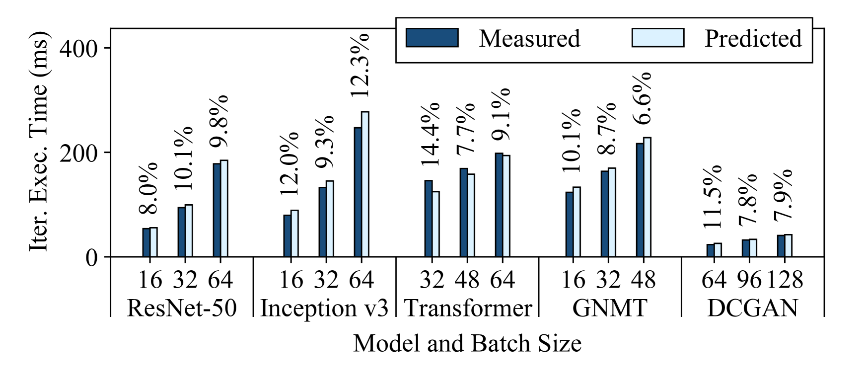
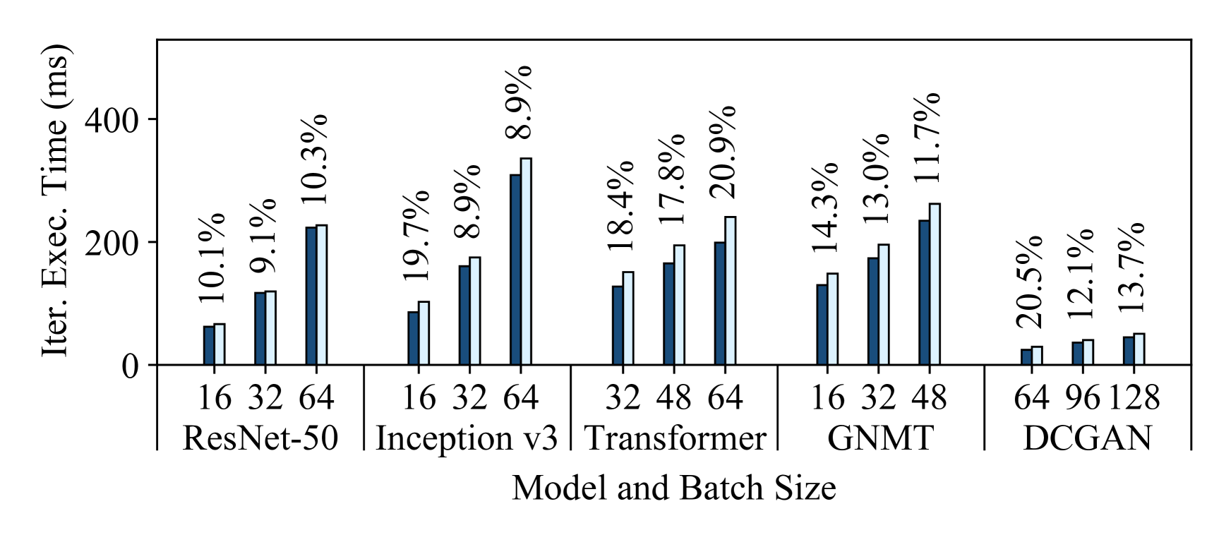
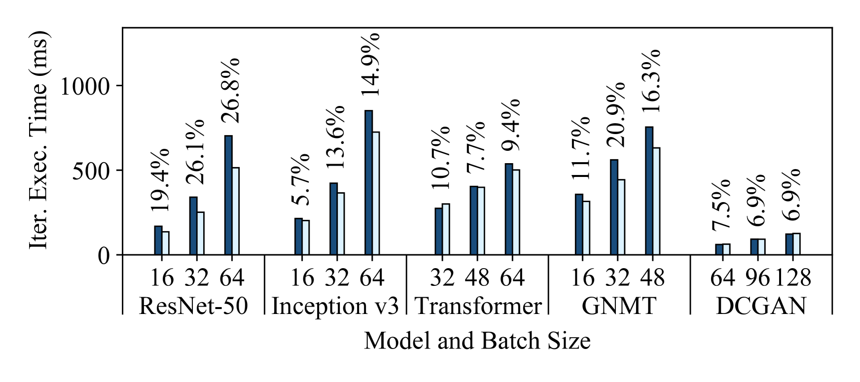
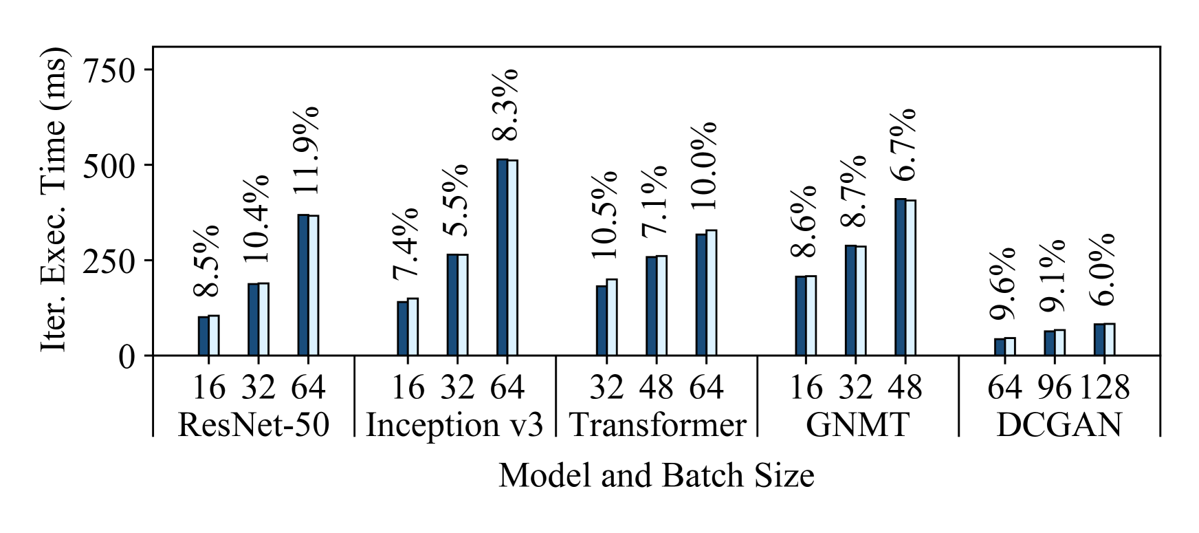
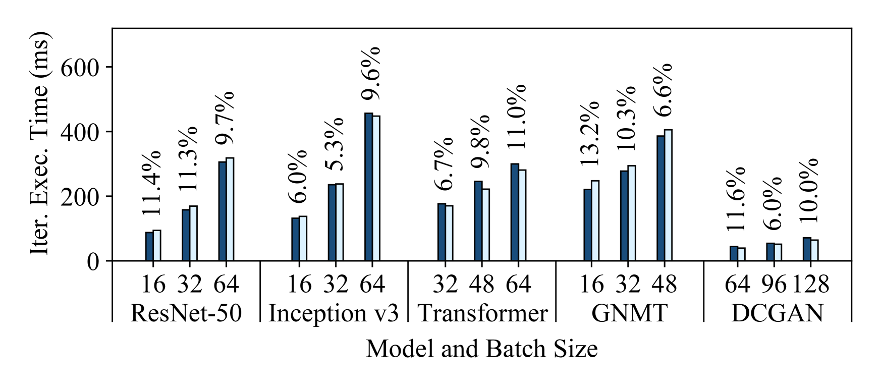
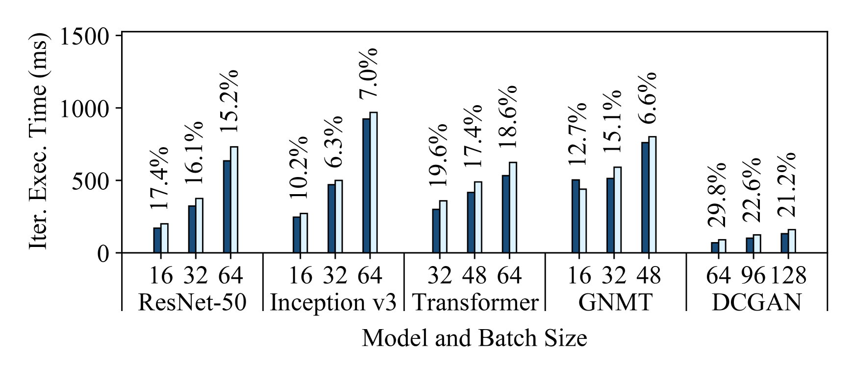
Figure 4 shows Habitat’s prediction errors for these aforementioned end-to-end predictions. Each subfigure shows the predictions for all five models on a specific destination GPU. We make predictions for three different batch sizes (shown on the figures) and plot both the predicted and measured iteration execution times. Since we consider all possible pairs of our six GPUs, for each destination GPU we plot the average predicted execution times among the five origin GPUs. Similarly, we show the average prediction error above each bar. From these figures, we can draw three major conclusions.

First, Habitat makes accurate end-to-end iteration execution time predictions since the average prediction error across all GPUs and models is 11.8%. The average prediction error across all ResNet-50, Inception v3, Transformer, GNMT, and DCGAN configurations are 13.4%, 9.5%, 12.6%, 11.2%, and 12.3% respectively.

Second, Habitat can predict the iteration execution time across GPU generations, which have different architectures, and across classes of GPUs. The GPUs we use span three generations (Pascal [63], Volta [67], and Turing [72]) and include desktop, professional workstation, and server-class GPUs.

Third, Habitat is general since it supports different types of DNN architectures. Habitat works with convolutional neural networks (e.g., ResNet-50, Inception v3, DCGAN), recurrent neural networks (e.g., GNMT), and other neural network architectures such as the attention-based Transformer. In particular, Habitat makes accurate predictions for ResNet, Inception, and DCGAN despite the significant differences in their architectures; ResNet has a “straight-line” computational graph, Inception has a large “fanout” in its graph, and DCGAN is a generative-adversarial model.

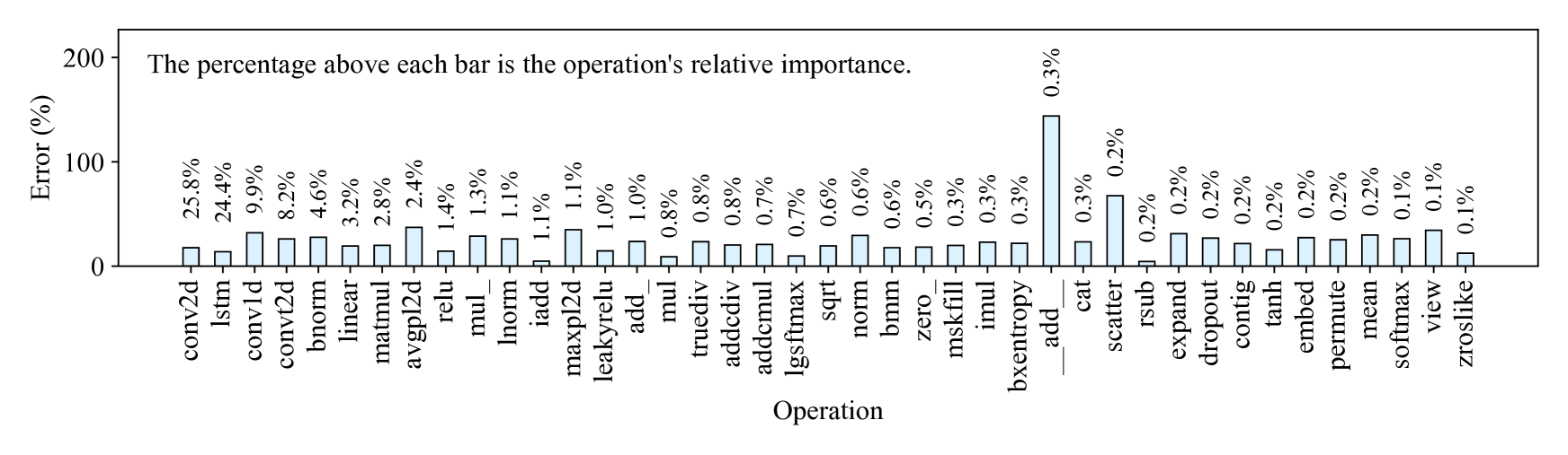
5.2.2 Prediction Error Breakdown

Figure 5 shows a breakdown of the prediction errors for the execution time of individual operations, which are listed on the $x$ -axis. The operations predicted using the MLP predictors are shown on the left (conv2d, lstm, bmm, and linear). Wave scaling is used to predict the rest of the operations. Above each bar, we also show the importance of each operation as a percentage of the iteration execution time, averaged across all five DNNs. The prediction errors are averaged among all pairs of the six GPUs that we evaluate and among ResNet-50, Inception v3, the Transformer, GNMT, and DCGAN. From this figure, we can draw two major conclusions.

First, MLP predictors can be used to make accurate predictions for kernel-varying operations as the average error among the conv2d, lstm, bmm, and linear operations is 18.0%. Second, wave scaling can make accurate predictions for important operations; the average error for wave scaling predictions is 29.8%. Although wave scaling’s predictions for some operations (e.g., __add__, scatter) have high errors, these operations do not make up a significant proportion of the training iteration execution time (having an overall importance of at most 0.3%).

5.2.3 Prediction Contribution Breakdown

We also examine how wave scaling and the MLPs each contribute to making Habitat’s end-to-end predictions. In our evaluation, Habitat uses wave scaling for 95% of the unique operations; it uses MLPs for the other 5%. In contrast, when looking at execution time, Habitat uses wave scaling to predict 46% of an iteration’s execution time on average; it uses MLPs for the other 54%.

These breakdowns show that both wave scaling and the MLPs contribute non-trivially to Habitat’s predictions—each is responsible for roughly half of an iteration’s execution time. Additionally, the unique operation breakdown shows that most operations are predicted using wave scaling. This observation highlights a strength of Habitat’s hybrid approach of using both wave scaling and MLPs: most operations can be automatically predicted using wave scaling; MLPs only need to be trained for a few kernel-varying operations.

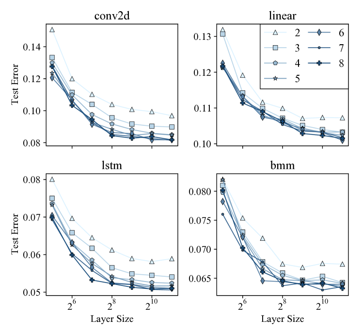
5.2.4 MLPs: How Many Layers?

In all our MLPs, we use eight hidden layers, each of size 1024. To better understand how the number of layers affects the MLPs’ prediction accuracy, we also conduct a sensitivity study where we vary the number of hidden layers in each MLP (2 to 8) along with their size (powers of two: $2^{5}$ to $2^{11}$ ). Figure 6 shows each MLP’s test mean absolute percentage error after being trained for 80 epochs. From this figure we can draw two major conclusions.

First, increasing the number of layers and their sizes leads to lower test errors. Increasing the size of each layer beyond $2^{9}$ seems to lead to diminishing returns on each operation. Second, the MLPs for all four operations appear to follow a similar test error trend. Based on these results, we can also conclude that using eight hidden layers is a reasonable choice.

5.3 Does Habitat Lead to Correct Decisions?

One of Habitat’s primary use cases is to help deep learning users make informed and cost-efficient GPU selections. In the following two case studies, we demonstrate how Habitat can make cost-efficiency predictions that empower users to make correct selections according to their needs.

5.3.1 Case Study 1: Should I Rent a Cloud GPU?

As mentioned in Section 1, one scenario a deep learning user may face is deciding whether to rent GPUs in the cloud for training or to stick with a GPU they already have locally (e.g., in their desktop). For example, suppose a user has a P4000 in their workstation and they want to decide whether to rent a P100, T4, or V100 in the cloud to train GNMT.

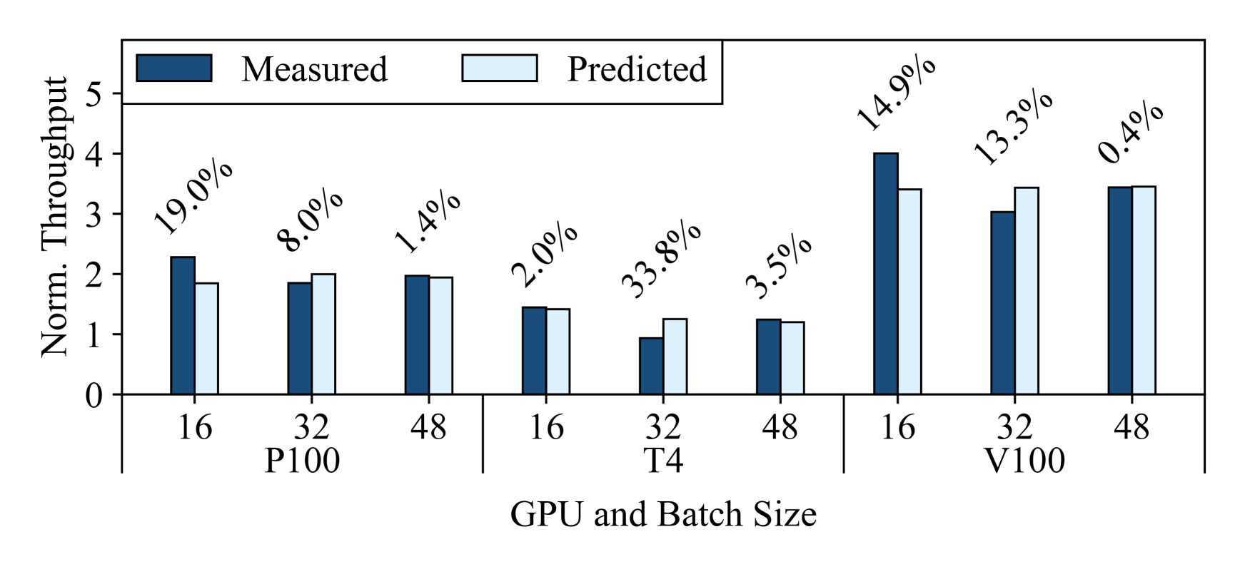
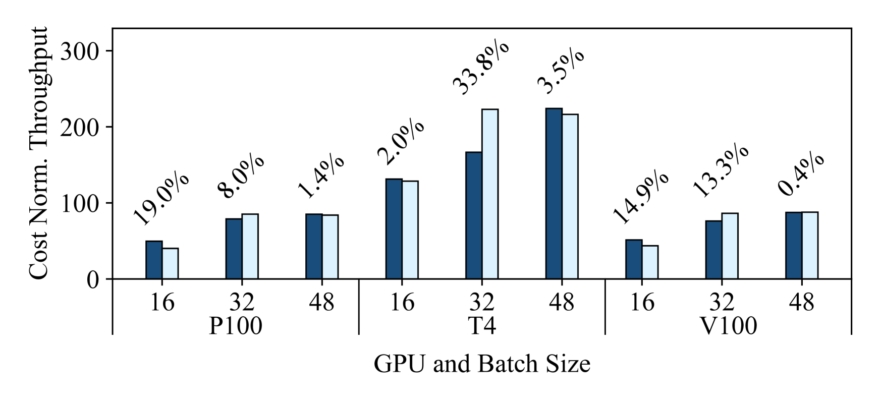
With Habitat, they can use their P4000 to make predictions about the computational performance of each cloud GPU to help them make this decision in an informed way. Figure 7(a) shows Habitat’s throughput predictions for GNMT for the P100, T4, and V100 normalized to the training throughput on the P4000. Additionally, Figure 7(b) shows Habitat’s predicted training throughputs normalized by each cloud GPU’s rental costs on Google Cloud as shown in Table 2. Note that (i) we make all these predictions with the P4000 as the origin device, (ii) we make our ground truth measurements on Google Cloud instances, and (iii) one can also use Habitat for a similar analysis for other cloud providers. From these results, the user can make two observations.

First, both the P100 and V100 offer training throughput speedups over the P4000 (up to $2.3\times$ and $4.0\times$ respectively) whereas the T4 offers marginal throughput speedups (up to $1.4\times$ ). However, second, the user would also discover that the T4 is more cost-efficient to rent when compared to the P100 and V100 as it has a higher cost-normalized throughput. Therefore, if the user wanted to optimize for maximum computational performance, they would likely choose the V100. But if they were not critically constrained by time and wanted to optimize for cost, sticking with the P4000 or renting a T4 would be a better choice.

Habitat makes these predictions accurately, with an average error of 10.7%. We also note that despite any prediction errors, Habitat still correctly predicts the relative ordering of these three GPUs in terms of their throughput and cost-normalized throughput. For example, in Figure 7(b), Habitat correctly predicts that the T4 offers the best cost-normalized throughput on all three batch sizes. These predictions therefore allow users to make correct decisions based on their needs (optimizing for cost or pure performance).

5.3.2 Case Study 2: Is the V100 Always Better?

In the previous case study, Habitat correctly predicts that the V100 provides the best performance despite not being the most cost-efficient to rent. This conclusion may lead a naïve user to believe that the V100 always provides better training throughput over other GPUs, given that it is the most advanced and expensive GPU available in the cloud to rent.⁸⁸8This is true except for the new A100s, which have only recently become publicly available in the cloud. In this case study, we show how Habitat can help a user recognize when the V100 does not offer significant performance benefits for their model.

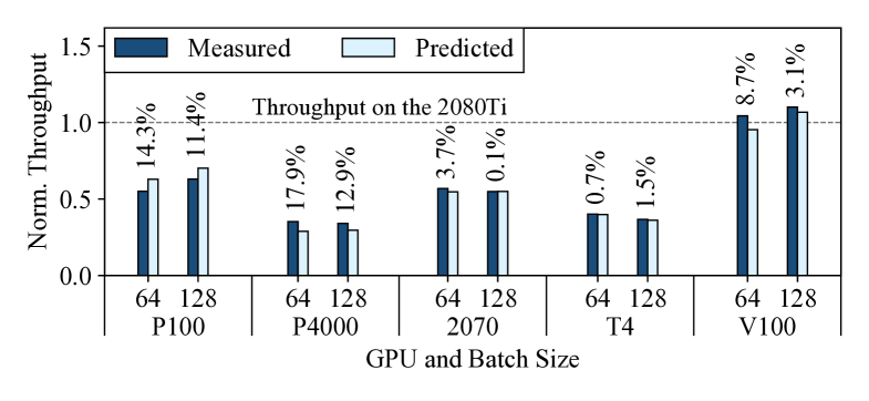
Suppose a user wants to train DCGAN and already has a 2080Ti that they can use. They want to find out if they should use a different GPU to get better computational performance (training throughput). They can use Habitat to predict the training throughput on other GPUs. Figure 8 shows Habitat’s throughput predictions along with the measured throughput, normalized to the 2080Ti’s training throughput. Note that we use a batch size of 64 as it is the default batch size in the DCGAN reference implementation [22] and 128 because it is the size reported by the authors in their paper [89].

From this figure, the user would conclude that they should stick to using their 2080Ti as the V100 would not be worth renting. The V100 offers marginal throughput improvements over the 2080Ti ( $1.1\times$ ) while the P100, P4000, 2070, and T4 all do not offer throughput improvements at all. The reason the V100 does not offer any significant benefits over the 2080Ti despite having more computational resources (Table 2) is that DCGAN is a “computationally lighter” model compared to GNMT and so it does not really benefit from a more powerful GPU. Habitat makes these predictions accurately, with an average error of 7.7%.

Summary.

These case studies show examples of situations where (i) the GPU offering the highest training throughput is not the same as the most cost-efficient GPU, and where (ii) the V100 does not offer significantly better performance when compared to a desktop-class GPU (the 2080Ti). Notably, in both case studies, Habitat correctly predicts each of these findings. As a result, deep learning researchers and practitioners can rely on Habitat to help them make correct cost-efficient GPU selections according to their needs.

6 Discussion

In this section, we discuss how Habitat can be extended to support additional (i) training setups, and (ii) deep learning frameworks. In doing so, we also highlight opportunities for future work and describe some challenges and opportunities associated with supporting additional hardware accelerators

6.1 Additional Training Setups

Habitat is designed to make accurate cross-GPU execution time predictions for DNN training. However, users may also face situations where they need performance predictions for more complex training setups such as (i) distributed training [25], (ii) mixed precision training [55], or (iii) needing predictions for batch sizes larger than what can fit on the origin GPU. In this subsection, we outline how Habitat could be extended to support these setups.

6.1.1 Distributed Training

Predicting the execution time of a distributed training iteration generally reduces to predicting (i) the computation time on the cluster’s GPUs, (ii) the communication time among the GPUs and/or nodes, and (iii) how the communication overlaps with the computation. For data parallel training [25], several prior works present techniques for predicting the data parallel iteration execution time given the execution time on a single GPU [110, 87, 88] (i.e., tasks (ii) and (iii)). Habitat’s computation predictions (task (i)) could be used as an input to these existing techniques.

For more complex distribution schemes such as model parallel [25] and pipeline parallel training [60, 40], Habitat could still be used for task (i), but the user would need to split up their model based on the distributed partitioning scheme before profiling it with Habitat. However, for tasks (ii) and (iii), new prediction techniques would need to be developed. This is something we leave to future work.

6.1.2 Mixed Precision Training

The Daydream paper [110] presents a technique for predicting the performance benefits of switching from single to mixed precision training on the same fixed GPU. If users want to know about the performance benefits of mixed precision training on a different GPU, they can use Daydream’s technique in conjunction with Habitat.

To show that this combined approach can work in practice, we use a P4000 to predict the execution time of a ResNet-50 mixed precision training iteration on the 2070 and 2080Ti.⁹⁹9We use the same experimental setup and batch sizes as described and shown in Section 5.1 and Figure 4. We compare our iteration execution time predictions against training iterations performed using PyTorch’s automatic mixed precision module. On the P4000, we first use Habitat to predict the single precision iteration execution time on the 2070 and 2080Ti. Then, we apply Daydream’s technique to translate these predicted single precision execution times into mixed precision execution times. We also repeat this experiment between the 2070 and 2080Ti. Overall, we find that this approach has an average error of 16.1% for predictions onto the 2070 and 2080Ti.

To distinguish between the errors introduced by Habitat versus Daydream, we also apply Daydream’s technique to the measured (i.e., ground truth) single precision iteration execution times. We find that Daydream’s technique alone has an average error of 10.7% for the 2070 and 2080Ti. Thus we believe the additional error introduced by also using Habitat is reasonable, given the extra functionality. So overall, we conclude that Habitat with Daydream should be able to effectively support mixed precision predictions on other GPUs.

6.1.3 Larger Batch Sizes

Recall that Habitat’s iteration execution time predictions are for a model and a specific batch size. This means that the origin GPU must be able to run a training iteration with the desired batch size (for Habitat’s profiling pass).

One potential approach to making predictions for batch sizes larger than what can run on the origin GPU is as follows. First, use Habitat to make iteration execution time predictions for multiple (e.g., three) different batch sizes that do fit on the origin GPU. Then, build a linear regression model on these predicted values to extrapolate to larger batch sizes. This approach is based on our prior work, where we observed an often linear relationship between the iteration execution time and batch size [107]. We leave the handling of models where only one batch size fits on the origin GPU to future work.

6.2 Additional Deep Learning Frameworks

Recall that Habitat predicts the execution time of operations using either (i) wave scaling or (ii) pre-trained MLPs, depending on whether the operation is kernel-alike or kernel-varying. Therefore, as long as Habitat has information about a DNN’s operations and their parameters (e.g., batch size, number of channels), Habitat will be able to apply its techniques to make execution time predictions for a different GPU. Ultimately this means that adding support for other deep learning frameworks (e.g., TensorFlow or MXNet) boils down to extracting the underlying operations that run during a training iteration and sending the operations to Habitat (i.e., extracting the computation graph). Since the other major deep learning frameworks (TensorFlow and MXNet) both already use computation graphs internally [1, 19], we believe that adding support for them would be straightforward to implement.

6.3 Additional Hardware Accelerators

As described in Section 1, there are also other hardware options available beyond GPUs that can be used for training (e.g., the TPU [45], AWS Trainium [10], and Gaudi [36]). Therefore, a natural opportunity for future work is to explore execution time predictions for these other hardware accelerators. We outline two challenges that arise when going beyond GPUs, as well as two examples of ways that Habitat’s guiding principles can be applied to these prediction tasks.

Challenges.

First, specialized deep learning accelerators may have a different hardware architecture when compared to GPUs—necessitating different performance modeling techniques. For example, the TPU uses a systolic array [45, 14] whereas GPUs are general-purpose SIMT processors [85]. Second, accelerators such as the TPU rely on tensor compilers (e.g., XLA [34] or JAX [13]) to produce executable code from the high-level DNN model code written by an end-user. The compiler may apply optimizations that change the operations. These changes make the high-level operation-based analysis that Habitat performs more difficult to realize.

Opportunities.

Despite these challenges, we believe that there are also opportunities to apply Habitat’s key idea of leveraging runtime-based information from one accelerator to predict the execution time on a different accelerator. For example, as of June 2021, Google makes two versions of the TPU available for rent (v2 and v3) [33] and has announced the v4 [51]. Execution times measured on the TPU v2 could potentially be used to make execution time predictions on the v3 and v4 and vice-versa. Similarly, assuming that the AWS Trainium also uses a systolic array,¹⁰¹⁰10The AWS Inferentia [9, 108], a related accelerator, uses a systolic array architecture [92]. So we believe that this is a reasonable assumption to make. it may also be possible to leverage execution time measurements on the TPU to make execution time predictions for the Trainium and vice-versa.

7 Related Work

The key difference between Habitat and existing DNN performance modeling techniques for GPUs [88, 46, 87] is in how Habitat makes execution time predictions. Habitat takes a hybrid runtime-based approach; it uses information recorded at runtime on one GPU along with hardware characteristics to scale the measured kernel execution times onto different GPUs through either (i) wave scaling, or (ii) pre-trained MLPs. In contrast, existing techniques use analytical models [88, 87] or rely entirely on machine learning techniques [46]. The key advantage of Habitat’s hybrid scaling approach is that wave scaling works “out of the box” for all kernel-alike operations (i.e., operations implemented using the same kernels on different GPUs). Ultimately, this advantage means that new analytical or machine learning models do not have to be developed each time a new kernel-alike operation is introduced.

DNN performance models for different hardware.

There exists prior work on performance models for DNN training on GPUs [88, 46, 87], CPUs [100], and TPUs [47]. As described above, Habitat is fundamentally different from these works because it takes a hybrid runtime-based approach when making execution time predictions. For example, Paleo [88] (i) makes DNN operation execution time predictions using analytical models based on the number of floating point operations (FLOPs) in a DNN operation, and (ii) uses heuristics to select the kernels used to implement kernel-varying operations (e.g., convolution). However, an operation’s execution time is not solely determined by its number of FLOPs, and using heuristics to select an analytical model cannot always capture kernel-varying operations correctly. This is because proprietary closed-source kernel libraries (e.g., cuDNN [74, 21], cuBLAS [77]) may select different kernel(s) to use by running benchmarks on the target GPU [44, 75].

Performance models for compilers.

A complementary body of work on performance modeling is motivated by the needs of compilers: predicting how different implementations of some high-level functionality perform on the same hardware. These models were developed to aid in compiling high-performance (i) graphics pipelines [2], (ii) CPU code [54], and (iii) tensor operators for deep learning accelerators [20, 47]. These models have fundamentally different goals compared to Habitat, which is a technique that predicts the performance of different GPUs running the same high-level code.

General scalability predictions.

Wave scaling is similar in spirit to ESTIMA [17], since both use the idea of making measurements on one system to make performance predictions for a different system. However, ESTIMA is a scalability predictor for CPU programs. Wave scaling instead targets GPU kernels, which run under a different execution model when compared to CPU programs.

Repetitiveness of DNN training.

Prior work leverages the repetitiveness of DNN training computation to optimize distributed training [43, 48, 60], schedule jobs in a cluster [103, 61, 18], and to apply DNN compiler optimizations [94]. The key difference between these works and Habitat is that they apply optimizations on the same hardware configuration. Habitat exploits the repetitiveness of DNN training to make performance predictions on different hardware configurations.

DNN benchmarking.

A body of prior work focuses on benchmarking DNN training [3, 109, 23, 53]. While these works provide DNN training performance insights, they do so only for a fixed set of DNNs and hardware configurations. In contrast, Habitat analyzes DNNs in general and provides performance predictions on different GPUs to help users make informed GPU selections.

8 Conclusion

We present Habitat: a new runtime-based library that uses wave scaling and MLPs as execution time predictors to help deep learning researchers and practitioners make informed cost-efficient decisions when selecting a GPU for DNN training. The key idea behind Habitat is to leverage information collected at runtime on one GPU to help predict the execution time of a DNN training iteration on a different GPU. We evaluate Habitat and find that it makes cross-GPU iteration execution time predictions with an overall average error of 11.8% on ResNet-50, Inception v3, the Transformer, GNMT, and DCGAN. Finally, we present two case studies where Habitat correctly predicts that (i) optimizing for cost-efficiency would lead to selecting a different GPU for GNMT, and (ii) that the V100 does not offer significant performance benefits over a common desktop-class GPU (the 2080Ti) for DCGAN. We have also open sourced Habitat (github.com/geoffxy/habitat) to benefit both the deep learning and systems communities [105, 106].

Acknowledgments

We thank our shepherd, Marco Canini, and the anonymous reviewers for their feedback. We also thank (in alphabetical order) Moshe Gabel, James Gleeson, Anand Jayarajan, Xiaodan Tan, Alexandra Tsvetkova, Shang Wang, Qiongsi Wu, and Hongyu Zhu. We thank all members of the EcoSystem research group for the stimulating research environment they provide. This work was supported by a QEII-GSST, Vector Scholarship in Artificial Intelligence, Snap Research Scholarship, and an NSERC Canada Graduate Scholarship – Master’s (CGS M). This work was also supported in part by the NSERC Discovery grant, the Canada Foundation for Innovation JELF grant, the Connaught Fund, an Amazon Research Award, and a Facebook Faculty Award. Computing resources used in this work were provided, in part, by the Province of Ontario, the Government of Canada through CIFAR, and companies sponsoring the Vector Institute www.vectorinstitute.ai/partners.

References

[1] Martín Abadi, Paul Barham, Jianmin Chen, Zhifeng Chen, Andy Davis, Jeffrey Dean, Matthieu Devin, Sanjay Ghemawat, Geoffrey Irving, Michael Isard, Manjunath Kudlur, Josh Levenberg, Rajat Monga, Sherry Moore, Derek G. Murray, Benoit Steiner, Paul Tucker, Vijay Vasudevan, Pete Warden, Martin Wicke, Yuan Yu, and Xiaoqiang Zheng. TensorFlow: A System for Large-Scale Machine Learning. In Proceedings of the 12th USENIX Symposium on Operating Systems Design and Implementation (OSDI’16), 2016.
[2] Andrew Adams, Karima Ma, Luke Anderson, Riyadh Baghdadi, Tzu-Mao Li, Michaël Gharbi, Benoit Steiner, Steven Johnson, Kayvon Fatahalian, Frédo Durand, and Jonathan Ragan-Kelley. Learning to Optimize Halide with Tree Search and Random Programs. ACM Transactions on Graphics (TOG), 38(4), 2019.
[3] Robert Adolf, Saketh Rama, Brandon Reagen, Gu-Yeon Wei, and David Brooks. Fathom: Reference Workloads for Modern Deep Learning Methods. In Proceedings of the 2016 IEEE International Symposium on Workload Characterization (IISWC’16), 2016.
[4] Advanced Micro Devices, Inc. HBM2 - High Bandwidth Memory-2, 2015. https://www.amd.com/system/files/documents/high-bandwidth-memory-hbm.pdf.
[5] Advanced Micro Devices, Inc. AMD Ryzen Threadripper 1950X Processor, 2017. https://www.amd.com/en/products/cpu/amd-ryzen-threadripper-1950x.
[6] Advanced Micro Devices, Inc. AMD EPYC™ 7371 Processor, 2020. https://www.amd.com/en/products/cpu/amd-epyc-7371.
[7] Amazon, Inc. Amazon EC2 Instance Types, 2020. https://aws.amazon.com/ec2/instance-types/.
[8] Amazon, Inc. Amazon SageMaker, 2021. https://aws.amazon.com/sagemaker/.
[9] Amazon, Inc. AWS Inferentia, 2021. https://aws.amazon.com/machine-learning/inferentia/.
[10] Amazon, Inc. AWS Trainium, 2021. https://aws.amazon.com/machine-learning/trainium/.
[11] Ondřej Bojar, Rajen Chatterjee, Christian Federmann, Yvette Graham, Barry Haddow, Matthias Huck, Antonio Jimeno Yepes, Philipp Koehn, Varvara Logacheva, Christof Monz, Matteo Negri, Aurelie Neveol, Mariana Neves, Martin Popel, Matt Post, Raphael Rubino, Carolina Scarton, Lucia Specia, Marco Turchi, Karin Verspoor, and Marcos Zampieri. Findings of the 2016 Conference on Machine Translation. In Proceedings of the First Conference on Machine Translation (WMT’16), 2016.
[12] Léon Bottou. Large-Scale Machine Learning with Stochastic Gradient Descent. In Proceedings of the 19th International Conference on Computational Statistics (COMPSTAT’10), 2010.
[13] James Bradbury, Roy Frostig, Peter Hawkins, Matthew James Johnson, Chris Leary, Dougal Maclaurin, George Necula, Adam Paszke, Jake VanderPlas, Skye Wanderman-Milne, and Qiao Zhang. JAX: Composable Transformations of Python+NumPy Programs, 2018. http://github.com/google/jax.
[14] Richard P Brent and Hsiang-Tsung Kung. Systolic VLSI Arrays for Polynomial GCD Computation. IEEE Transactions on Computers, 100(8):731–736, 1984.
[15] Canonical Ltd. Ubuntu 18.04 LTS (Bionic Beaver), 2018. http://releases.ubuntu.com/18.04/.
[16] Cerebras. Cerebras, 2020. https://www.cerebras.net.
[17] Georgios Chatzopoulos, Aleksandar Dragojević, and Rachid Guerraoui. ESTIMA: Extrapolating Scalability of in-Memory Applications. In Proceedings of the 21st ACM SIGPLAN Symposium on Principles and Practice of Parallel Programming (PPoPP’16), 2016.
[18] Shubham Chaudhary, Ramachandran Ramjee, Muthian Sivathanu, Nipun Kwatra, and Srinidhi Viswanatha. Balancing Efficiency and Fairness in Heterogeneous GPU Clusters for Deep Learning. In Proceedings of the 15th European Conference on Computer Systems (EuroSys’20), 2020.
[19] Tianqi Chen, Mu Li, Yutian Li, Min Lin, Naiyan Wang, Minjie Wang, Tianjun Xiao, Bing Xu, Chiyuan Zhang, and Zheng Zhang. MXNet: A Flexible and Efficient Machine Learning Library for Heterogeneous Distributed Systems. In Proceedings of the 2016 NeurIPS Workshop on Machine Learning Systems, 2016.
[20] Tianqi Chen, Lianmin Zheng, Eddie Yan, Ziheng Jiang, Thierry Moreau, Luis Ceze, Carlos Guestrin, and Arvind Krishnamurthy. Learning to Optimize Tensor Programs. In Advances in Neural Information Processing Systems 31 (NeurIPS’18), 2018.
[21] Sharan Chetlur, Cliff Woolley, Philippe Vandermersch, Jonathan Cohen, John Tran, Bryan Catanzaro, and Evan Shelhamer. cuDNN: Efficient Primitives for Deep Learning. arXiv, abs/1410.0759, 2014.
[22] Soumith Chintala. Deep Convolution Generative Adversarial Networks, 2020. https://github.com/pytorch/examples/tree/master/dcgan/.
[23] Cody Coleman, Deepak Narayanan, Daniel Kang, Tian Zhao, Jian Zhang, Luigi Nardi, Peter Bailis, Kunle Olukotun, Chris Ré, and Matei Zaharia. DAWNBench: An End-to-End Deep Learning Benchmark and Competition. In Proceedings of the NeurIPS Workshop on Machine Learning Systems, 2017.
[24] PyTorch Contributors. torchvision, 2021. https://github.com/pytorch/vision.
[25] Jeffrey Dean, Greg S. Corrado, Rajat Monga, Kai Chen, Matthieu Devin, Quoc V. Le, Mark Z. Mao, Marc’Aurelio Ranzato, Andrew Senior, Paul Tucker, Ke Yang, and Andrew Y. Ng. Large Scale Distributed Deep Networks. In Advances in Neural Information Processing Systems 25 (NeurIPS’12), 2012.
[26] Jacob Devlin, Ming-Wei Chang, Kenton Lee, and Kristina Toutanova. BERT: Pre-training of Deep Bidirectional Transformers for Language Understanding. In Proceedings of the 2019 Annual Conference of the North American Chapter of the Association for Computational Linguistics (NAACL’19), 2019.
[27] Docker, Inc. Docker, 2020. https://www.docker.com/.
[28] Peter N. Glaskowsky. NVIDIA’s Fermi: The First Complete GPU Computing Architecture. Whitepaper, NVIDIA, 2009.
[29] Ian Goodfellow, Yoshua Bengio, and Aaron Courville. Deep Learning. MIT Press, 2016. http://www.deeplearningbook.org.
[30] Google, Inc. Google Cloud N1 Machine Types, 2020. https://cloud.google.com/compute/docs/machine-types#n1_machine_types.
[31] Google, Inc. GPUs on Compute Engine, 2020. https://cloud.google.com/compute/docs/gpus.
[32] Google, Inc. Google Cloud Vertex AI, 2021. https://cloud.google.com/vertex-ai/.
[33] Google, Inc. Supported TPU Versions, 2021. https://cloud.google.com/tpu/docs/supported-tpu-versions.
[34] Google, Inc. XLA: Optimizing Compiler for Machine Learning, 2021. https://www.tensorflow.org/xla.
[35] Graphcore. Graphcore, 2020. https://www.graphcore.ai.
[36] Habana Labs. Habana Labs, 2020. https://habana.ai.
[37] Kaiming He, Xiangyu Zhang, Shaoqing Ren, and Jian Sun. Deep Residual Learning for Image Recognition. In Proceedings of the IEEE Conference on Computer Vision and Pattern Recognition (CVPR’16), 2016.
[38] Sepp Hochreiter and Jürgen Schmidhuber. Long Short-Term Memory. Neural Computation, 9(8):1735–1780, 1997.
[39] Gao Huang, Zhuang Liu, Laurens van der Maaten, and Kilian Q Weinberger. Densely Connected Convolutional Networks. In Proceedings of the 2017 IEEE Conference on Computer Vision and Pattern Recognition (CVPR’17), 2017.
[40] Yanping Huang, Youlong Cheng, Ankur Bapna, Orhan Firat, Dehao Chen, Mia Xu Chen, HyoukJoong Lee, Jiquan Ngiam, Quoc V. Le, Yonghui Wu, and Zhifeng Chen. GPipe: Efficient Training of Giant Neural Networks using Pipeline Parallelism. In Advances in Neural Information Processing Systems 32 (NeurIPS’19), 2019.
[41] Intel Corporation. Intel Xeon Processor E5-2680, 2020. https://ark.intel.com/content/www/us/en/ark/products/91754/intel-xeon-processor-e5-2680-v4-35m-cache-2-40-ghz.html.
[42] Sergey Ioffe and Christian Szegedy. Batch Normalization: Accelerating Deep Network Training by Reducing Internal Covariate Shift. In Proceedings of the 32nd International Conference on International Conference on Machine Learning (ICML’15), 2015.
[43] Zhihao Jia, Matei Zaharia, and Alex Aiken. Beyond Data and Model Parallelism for Deep Neural Networks. In Proceedings of the 2nd Conference on Systems and Machine Learning (MLSys’19), 2019.
[44] Marc Jorda, Pedro Valero-Lara, and Antonio J Peña. Performance Evaluation of cuDNN Convolution Algorithms on NVIDIA Volta GPUs. IEEE Access, 7:70461–70473, 2019.
[45] Norman P. Jouppi, Cliff Young, Nishant Patil, David Patterson, Gaurav Agrawal, Raminder Bajwa, Sarah Bates, Suresh Bhatia, Nan Boden, Al Borchers, Rick Boyle, Pierre-luc Cantin, Clifford Chao, Chris Clark, Jeremy Coriell, Mike Daley, Matt Dau, Jeffrey Dean, Ben Gelb, Tara Vazir Ghaemmaghami, Rajendra Gottipati, William Gulland, Robert Hagmann, C. Richard Ho, Doug Hogberg, John Hu, Robert Hundt, Dan Hurt, Julian Ibarz, Aaron Jaffey, Alek Jaworski, Alexander Kaplan, Harshit Khaitan, Daniel Killebrew, Andy Koch, Naveen Kumar, Steve Lacy, James Laudon, James Law, Diemthu Le, Chris Leary, Zhuyuan Liu, Kyle Lucke, Alan Lundin, Gordon MacKean, Adriana Maggiore, Maire Mahony, Kieran Miller, Rahul Nagarajan, Ravi Narayanaswami, Ray Ni, Kathy Nix, Thomas Norrie, Mark Omernick, Narayana Penukonda, Andy Phelps, Jonathan Ross, Matt Ross, Amir Salek, Emad Samadiani, Chris Severn, Gregory Sizikov, Matthew Snelham, Jed Souter, Dan Steinberg, Andy Swing, Mercedes Tan, Gregory Thorson, Bo Tian, Horia Toma, Erick Tuttle, Vijay Vasudevan, Richard Walter, Walter Wang, Eric Wilcox, and Doe Hyun Yoon. In-Datacenter Performance Analysis of a Tensor Processing Unit. In Proceedings of the 44th Annual International Symposium on Computer Architecture (ISCA’17), 2017.
[46] Daniel Justus, John Brennan, Stephen Bonner, and Andrew Stephen McGough. Predicting the Computational Cost of Deep Learning Models. In Proceedings of the 2018 IEEE Conference on Big Data (BigData’18), 2018.
[47] Samuel J. Kaufman, Phitchaya Mangpo Phothilimthana, Yanqi Zhou, Charith Mendis, Sudip Roy, Amit Sabne, and Mike Burrows. A Learned Performance Model for Tensor Processing Units. In Proceedings of the 4th Conference on Machine Learning and Systems (MLSys’21), 2021.
[48] Soojeong Kim, Gyeong-In Yu, Hojin Park, Sungwoo Cho, Eunji Jeong, Hyeonmin Ha, Sanha Lee, Joo Seong Jeong, and Byung-Gon Chun. Parallax: Sparsity-aware Data Parallel Training of Deep Neural Networks. In Proceedings of the 14th EuroSys Conference (EuroSys’19), 2019.
[49] Diederik P. Kingma and Jimmy Ba. Adam: A Method for Stochastic Optimization. In Proceedings of the 3rd International Conference for Learning Representations (ICLR’15), 2015.
[50] Alex Krizhevsky, Ilya Sutskever, and Geoffrey E Hinton. ImageNet Classification with Deep Convolutional Neural Networks. In Advances in Neural Information Processing Systems 25 (NeurIPS’12), 2012.
[51] Naveen Kumar. Google breaks AI performance records in MLPerf with world’s fastest training supercomputer, 2020. https://cloud.google.com/blog/products/ai-machine-learning/google-breaks-ai-performance-records-in-mlperf-with-worlds-fastest-training-supercomputer.
[52] Lambda Labs Inc. Lambda: Deep Learning Workstations, Servers, Laptops, 2020. https://lambdalabs.com.
[53] Peter Mattson, Christine Cheng, Cody Coleman, Greg Diamos, Paulius Micikevicius, David Patterson, Hanlin Tang, Gu-Yeon Wei, Peter Bailis, Victor Bittorf, David Brooks, Dehao Chen, Debojyoti Dutta, Udit Gupta, Kim Hazelwood, Andrew Hock, Xinyuan Huang, Bill Jia, Daniel Kang, David Kanter, Naveen Kumar, Jeffery Liao, Guokai Ma, Deepak Narayanan, Tayo Oguntebi, Gennady Pekhimenko, Lillian Pentecost, Vijay Janapa Reddi, Taylor Robie, Tom St. John, Carole-Jean Wu, Lingjie Xu, Cliff Young, and Matei Zaharia. MLPerf Training Benchmark. In Proceedings of the 3rd Conference on Machine Learning and Systems (MLSys’20), 2020.
[54] Charith Mendis, Alex Renda, Saman Amarasinghe, and Michael Carbin. Ithemal: Accurate, Portable and Fast Basic Block Throughput Estimation using Deep Neural Networks. In Proceedings of the 36th International Conference on Machine Learning (ICML’19), 2019.
[55] Paulius Micikevicius, Sharan Narang, Jonah Alben, Gregory F. Diamos, Erich Elsen, David García, Boris Ginsburg, Michael Houston, Oleksii Kuchaiev, Ganesh Venkatesh, and Hao Wu. Mixed Precision Training. In Proceedings of the 6th International Conference on Learning Representations (ICLR’18), 2018.
[56] Micron Technology, Inc. GDDR5, 2015. https://www.micron.com/products/graphics-memory/gddr5.
[57] Micron Technology, Inc. GDDR6, 2017. https://www.micron.com/products/graphics-memory/gddr6.
[58] Microsoft Corporation. Azure Machine Learning, 2021. https://azure.microsoft.com/services/machine-learning/.
[59] Ioannis Mitliagkas, Ce Zhang, Stefan Hadjis, and Christopher Ré. Asynchrony Begets Momentum, with an Application to Deep Learning. In 54th Annual Allerton Conference on Communication, Control, and Computing (Allerton’16), 2016.
[60] Deepak Narayanan, Aaron Harlap, Amar Phanishayee, Vivek Seshadri, Nikhil Devanur, Gregory R. Ganger, Phillip B. Gibbons, and Matei Zaharia. PipeDream: Generalized Pipeline Parallelism for DNN Training. In Proceedings of the 27th Symposium on Operating Systems Principles (SOSP’19), 2019.
[61] Deepak Narayanan, Keshav Santhanam, Fiodar Kazhamiaka, Amar Phanishayee, and Matei Zaharia. Heterogeneity-Aware Cluster Scheduling Policies for Deep Learning Workloads. In Proceedings of the 14th USENIX Symposium on Operating Systems Design and Implementation (OSDI’20), 2020.
[62] NVIDIA Corporation. NVIDIA Pascal P100, 2016. https://images.nvidia.com/content/tesla/pdf/nvidia-tesla-p100-PCIe-datasheet.pdf.
[63] NVIDIA Corporation. NVIDIA Tesla P100. Whitepaper, NVIDIA, 2016.
[64] NVIDIA Corporation. NVIDIA GeForce GTX 1080Ti, 2017. https://www.nvidia.com/en-us/geforce/products/10series/geforce-gtx-1080-ti.
[65] NVIDIA Corporation. NVIDIA Quadro P4000, 2017. https://www.pny.com/nvidia-quadro-p4000.
[66] NVIDIA Corporation. NVIDIA Tesla V100, 2017. https://images.nvidia.com/content/technologies/volta/pdf/tesla-volta-v100-datasheet-letter-fnl-web.pdf.
[67] NVIDIA Corporation. NVIDIA Tesla V100. Whitepaper, NVIDIA, 2017.
[68] NVIDIA Corporation. NVIDIA TITAN Xp, 2017. https://www.nvidia.com/en-us/titan/titan-xp.
[69] NVIDIA Corporation. NVIDIA GeForce RTX 2070, 2018. https://www.nvidia.com/en-us/geforce/graphics-cards/rtx-2070.
[70] NVIDIA Corporation. NVIDIA GeForce RTX 2080Ti, 2018. https://www.nvidia.com/en-us/geforce/graphics-cards/rtx-2080-ti/.
[71] NVIDIA Corporation. NVIDIA Tesla T4, 2018. https://www.nvidia.com/content/dam/en-zz/Solutions/Data-Center/tesla-t4/t4-tensor-core-datasheet-951643.pdf.
[72] NVIDIA Corporation. NVIDIA Turing Architecture. Whitepaper, NVIDIA, 2018. https://www.nvidia.com/content/dam/en-zz/Solutions/design-visualization/technologies/turing-architecture/NVIDIA-Turing-Architecture-Whitepaper.pdf.
[73] NVIDIA Corporation. CUDA Runtime API – Event Management, 2019. https://docs.nvidia.com/cuda/cuda-runtime-api/group__CUDART__EVENT.html.
[74] NVIDIA Corporation. cuDNN Developer Guide, 2019. https://docs.nvidia.com/deeplearning/sdk/cudnn-developer-guide/index.html.
[75] NVIDIA Corporation. cuDNN Developer Guide: cudnnFindConvolutionForwardAlgorithm, 2019. https://docs.nvidia.com/deeplearning/sdk/cudnn-developer-guide/index.html#cudnnFindConvolutionForwardAlgorithm.
[76] NVIDIA Corporation. CUPTI Documentation, 2019. https://docs.nvidia.com/cupti/Cupti/index.html.
[77] NVIDIA Corporation. cuBLAS: Dense Linear Algebra on GPUs, 2020. https://developer.nvidia.com/cublas.
[78] NVIDIA Corporation. NVIDIA A100, 2020. https://www.nvidia.com/en-us/data-center/a100.
[79] NVIDIA Corporation. NVIDIA Ampere Architecture In-Depth, 2020. https://developer.nvidia.com/blog/nvidia-ampere-architecture-in-depth/.
[80] NVIDIA Corporation. NVIDIA CUDA Toolkit, 2020. https://developer.nvidia.com/cuda-toolkit.
[81] NVIDIA Corporation. NVIDIA Data Center Deep Learning Product Performance, 2020. https://developer.nvidia.com/deep-learning-performance-training-inference.
[82] NVIDIA Corporation. NVIDIA GeForce RTX 3090, 2020. https://www.nvidia.com/en-us/geforce/graphics-cards/30-series/rtx-3090/.
[83] NVIDIA Corporation. NVIDIA GPU Cloud Virtual Machine Image Release Notes, 2020. https://docs.nvidia.com/ngc/ngc-ami-release-notes/.
[84] NVIDIA Corporation. Quadro RTX 6000 Graphics Card, 2020. https://www.nvidia.com/en-us/design-visualization/quadro/rtx-6000/.
[85] NVIDIA Corporation. CUDA Programming Guide, 2021. https://docs.nvidia.com/cuda/cuda-c-programming-guide/index.html.
[86] Adam Paszke, Sam Gross, Francisco Massa, Adam Lerer, James Bradbury, Gregory Chanan, Trevor Killeen, Zeming Lin, Natalia Gimelshein, Luca Antiga, Alban Desmaison, Andreas Köpf, Edward Yang, Zach DeVito, Martin Raison, Alykhan Tejani, Sasank Chilamkurthy, Benoit Steiner, Lu Fang, Junjie Bai, and Soumith Chintala. PyTorch: An Imperative Style, High-Performance Deep Learning Library. In Advances in Neural Information Processing Systems 32 (NeurIPS’19), 2019.
[87] Ziqian Pei, Chensheng Li, Xiaowei Qin, Xiaohui Chen, and Guo Wei. Iteration Time Prediction for CNN in Multi-GPU Platform: Modeling and Analysis. IEEE Access, 7:64788–64797, 2019.
[88] Hang Qi, Evan R. Sparks, and Ameet Talwalkar. Paleo: A Performance Model for Deep Neural Networks. In Proceedings of the 5th International Conference on Learning Representations (ICLR’17), 2017.
[89] Alec Radford, Luke Metz, and Soumith Chintala. Unsupervised Representation Learning with Deep Convolutional Generative Adversarial Networks. In Proceedings of the 4th International Conference on Learning Representations (ICLR’16), 2016.
[90] D. E. Rumelhart, G. E. Hinton, and R. J. Williams. Parallel Distributed Processing: Explorations in the Microstructure of Cognition, Vol. 1. MIT Press, 1986.
[91] Olga Russakovsky, Jia Deng, Hao Su, Jonathan Krause, Sanjeev Satheesh, Sean Ma, Zhiheng Huang, Andrej Karpathy, Aditya Khosla, Michael Bernstein, Alexander C. Berg, and Li Fei-Fei. ImageNet Large Scale Visual Recognition Challenge. International Journal of Computer Vision (IJCV), 115(3):211–252, 2015.
[92] Julien Simon. Announcing availability of Inf1 instances in Amazon SageMaker for high performance and cost-effective machine learning inference, 2020. https://aws.amazon.com/blogs/machine-learning/announcing-availability-of-inf1-instances-in-amazon-sagemaker-for-high-performance-and-cost-effective-machine-learning-inference/.
[93] Karen Simonyan and Andrew Zisserman. Very Deep Convolutional Networks for Large-Scale Image Recognition. In Proceedings of the 3rd International Conference on Learning Representations (ICLR’15), 2015.
[94] Muthian Sivathanu, Tapan Chugh, Sanjay S. Singapuram, and Lidong Zhou. Astra: Exploiting Predictability to Optimize Deep Learning. In Proceedings of the 24th International Conference on Architectural Support for Programming Languages and Operating Systems (ASPLOS’19), 2019.
[95] Emma Strubell, Ananya Ganesh, and Andrew McCallum. Energy and Policy Considerations for Deep Learning in NLP. In Proceedings of the 57th Annual Meeting of the Association for Computational Linguistics (ACL’19), 2019.
[96] Ilya Sutskever, Oriol Vinyals, and Quoc V Le. Sequence to Sequence Learning with Neural Networks. In Proceedings of Advances in Neural Information Processing Systems 27 (NeurIPS’14), 2014.
[97] Christian Szegedy, Vincent Vanhoucke, Sergey Ioffe, Jonathon Shlens, and Zbigniew Wojna. Rethinking the Inception Architecture for Computer Vision. arXiv, abs/1512.00567, 2015.
[98] TechPowerUp. TechPowerUp GPU Database (P4000 and 2070), 2020. https://www.techpowerup.com/gpu-specs/.
[99] Ashish Vaswani, Noam Shazeer, Niki Parmar, Jakob Uszkoreit, Llion Jones, Aidan N Gomez, Lukasz Kaiser, and Illia Polosukhin. Attention is All You Need. In Advances in Neural Information Processing Systems 30 (NeurIPS’17), 2017.
[100] Andre Viebke, Sabri Pllana, Suejb Memeti, and Joanna Kolodziej. Performance Modelling of Deep Learning on Intel Many Integrated Core Architectures. arXiv, abs/1906.01992, 2019.
[101] Samuel Williams, Andrew Waterman, and David Patterson. Roofline: An Insightful Visual Performance Model for Floating-Point Programs and Multicore Architectures. Communications of the ACM (CACM), 52(4):65–76, 2009.
[102] Yonghui Wu, Mike Schuster, Zhifeng Chen, Quoc V. Le, Mohammad Norouzi, Wolfgang Macherey, Maxim Krikun, Yuan Cao, Qin Gao, Klaus Macherey, Jeff Klingner, Apurva Shah, Melvin Johnson, Xiaobing Liu, Łukasz Kaiser, Stephan Gouws, Yoshikiyo Kato, Taku Kudo, Hideto Kazawa, Keith Stevens, George Kurian, Nishant Patil, Wei Wang, Cliff Young, Jason Smith, Jason Riesa, Alex Rudnick, Oriol Vinyals, Greg Corrado, Macduff Hughes, and Jeffrey Dean. Google’s Neural Machine Translation System: Bridging the Gap between Human and Machine Translation. arXiv, abs/1609.08144, 2016.
[103] Wencong Xiao, Romil Bhardwaj, Ramachandran Ramjee, Muthian Sivathanu, Nipun Kwatra, Zhenhua Han, Pratyush Patel, Xuan Peng, Hanyu Zhao, Quanlu Zhang, Fan Yang, and Lidong Zhou. Gandiva: Introspective Cluster Scheduling for Deep Learning. In Proceedings of the 13th Symposium on Operating Systems Design and Implementation (OSDI’18), 2018.
[104] Fisher Yu, Yinda Zhang, Shuran Song, Ari Seff, and Jianxiong Xiao. LSUN: Construction of a Large-scale Image Dataset using Deep Learning with Humans in the Loop. arXiv, abs/1506.03365, 2015.
[105] Geoffrey X. Yu, Yubo Gao, Pavel Golikov, and Gennady Pekhimenko. Habitat: A Runtime-Based Computational Performance Predictor for Deep Neural Network Training (Code), 2021. https://doi.org/10.5281/zenodo.4885489.
[106] Geoffrey X. Yu, Yubo Gao, Pavel Golikov, and Gennady Pekhimenko. Habitat Pre-Trained Models and Kernel Metadata, 2021. https://doi.org/10.5281/zenodo.4876277.
[107] Geoffrey X. Yu, Tovi Grossman, and Gennady Pekhimenko. Skyline: Interactive In-Editor Computational Performance Profiling for Deep Neural Network Training. In Proceedings of the 33rd ACM Symposium on User Interface Software and Technology (UIST’20), 2020.
[108] Hongbin Zheng, Sejong Oh, Huiqing Wang, Preston Briggs, Jiading Gai, Animesh Jain, Yizhi Liu, Rich Heaton, Randy Huang, and Yida Wang. Optimizing Memory-Access Patterns for Deep Learning Accelerators. In Proceedings of the 2nd Compilers for Machine Learning Workshop at CGO 2020 (C4ML’20), 2020.
[109] Hongyu Zhu, Mohamed Akrout, Bojian Zheng, Andrew Pelegris, Amar Phanishayee, Bianca Schroeder, and Gennady Pekhimenko. Benchmarking and Analyzing Deep Neural Network Training. In Proceedings of the 2018 IEEE International Symposium on Workload Characterization (IISWC’18), 2018.
[110] Hongyu Zhu, Amar Phanishayee, and Gennady Pekhimenko. Daydream: Accurately Estimating the Efficacy of Optimizations for DNN Training. In Proceedings of the 2020 USENIX Annual Technical Conference (USENIX ATC’20), 2020.

A Runtime-Based Computational Performance Predictor for Deep Neural Network Training

Abstract

1 Introduction

2 Why Predict the Computational Training Performance of DNNs on Different GPUs?

2.1 Background on DNN Training

Training.

Computational performance.

2.2 Why Not Measure Performance Directly?

2.3 Why Not Apply Heuristics?

2.4 Why Not Use Benchmarks?

2.5 Why Not Always Use the “Best” GPU?

Summary.

3 Habitat

3.1 Key Observations

Observation 1: Repetitive computation.

Observation 2: Common building blocks among DNNs.

Observation 3: Runtime information available.

3.2 Habitat Overview

3.3 Wave Scaling

3.4 MLP Predictors

Input features.

Model architecture.

4 Implementation Details

4.1 Extracting Runtime Metadata

Execution time.

Kernel metadata and metrics.

4.2 Selecting Gamma (γ\gamma)

Roofline model.

Selecting γ\gamma.

Practical optimizations.

4.3 MLPs: Data and Training

4.3.1 Data Collection

2D convolutions.

LSTMs.

Batched matrix multiply (bmm).

Linear layers.

4.3.2 Data Preprocessing

4.3.3 Training

5 Evaluation

5.1 Methodology

Hardware.

Runtime environment.

Models and datasets.

Metrics.

Measurements.

5.2 How Accurate are Habitat’s Predictions?

5.2.1 End-to-End Prediction Accuracy

5.2.2 Prediction Error Breakdown

5.2.3 Prediction Contribution Breakdown

5.2.4 MLPs: How Many Layers?

5.3 Does Habitat Lead to Correct Decisions?

5.3.1 Case Study 1: Should I Rent a Cloud GPU?

5.3.2 Case Study 2: Is the V100 Always Better?

Summary.

6 Discussion

6.1 Additional Training Setups

6.1.1 Distributed Training

6.1.2 Mixed Precision Training

6.1.3 Larger Batch Sizes

6.2 Additional Deep Learning Frameworks

6.3 Additional Hardware Accelerators

Challenges.

Opportunities.

7 Related Work

DNN performance models for different hardware.

Performance models for compilers.

General scalability predictions.

Repetitiveness of DNN training.

DNN benchmarking.

8 Conclusion

Acknowledgments

References

A Runtime-Based Computational Performance Predictor for
Deep Neural Network Training

4.2 Selecting Gamma ( $\gamma$ )

Selecting $\gamma$ .