A Sample Document\supportSupport information of the article.
Abstract
The abstract should summarize the contents of the paper. It should be clear, descriptive, self-explanatory and not longer than 200 words. It should also be suitable for publication in abstracting services. Please avoid using math formulas as much as possible.
This is a sample input file. Comparing it with the output it generates can show you how to produce a simple document of your own.
keywords:
[class=MSC]keywords:
2010.00000 \startlocaldefs \endlocaldefs
and
t1Some comment t2First supporter of the project t3Second supporter of the project
1 Ordinary text
The ends of words and sentences are marked by spaces. It doesn’t matter how many spaces you type; one is as good as 100. The end of a line counts as a space.
One or more blank lines denote the end of a paragraph.
Since any number of consecutive spaces are treated like a single one, the formatting of the input file makes no difference to TeX, but it makes a difference to you. When you use LaTeX, making your input file as easy to read as possible will be a great help as you write your document and when you change it. This sample file shows how you can add comments to your own input file.
Because printing is different from typewriting, there are a number of things that you have to do differently when preparing an input file than if you were just typing the document directly. Quotation marks like “this” have to be handled specially, as do quotes within quotes: “ ‘this’ is what I just wrote, not ‘that’ ”.
Dashes come in three sizes: an intra-word dash, a medium dash for number ranges like 1–2, and a punctuation dash—like this.
A sentence-ending space should be larger than the space between words within a sentence. You sometimes have to type special commands in conjunction with punctuation characters to get this right, as in the following sentence. Gnats, gnus, etc. all begin with G. You should check the spaces after periods when reading your output to make sure you haven’t forgotten any special cases. Generating an ellipsis … with the right spacing around the periods requires a special command.
TeX interprets some common characters as commands, so you must type special commands to generate them. These characters include the following: & % # { and }.
In printing, text is emphasized by using an italic type style.
A long segment of text can also be emphasized in this way. Text within such a segment given additional emphasis with Roman type. Italic type loses its ability to emphasize and become simply distracting when used excessively.
It is sometimes necessary to prevent TeX from breaking a line where it might otherwise do so. This may be at a space, as between the “Mr.” and “Jones” in “Mr. Jones”, or within a word—especially when the word is a symbol like itemnum that makes little sense when hyphenated across lines.
TeX is good at typesetting mathematical formulas like or . Remember that a letter like is a formula when it denotes a mathematical symbol, and should be treated as one.
2 Notes
Footnotes111This is an example of a footnote. pose no problem222And another one.
3 Displayed text
Text is displayed by indenting it from the left margin. Quotations are commonly displayed. There are short quotations
This is a short a quotation. It consists of a single paragraph of text. There is no paragraph indentation.
and longer ones.
This is a longer quotation. It consists of two paragraphs of text. The beginning of each paragraph is indicated by an extra indentation.
This is the second paragraph of the quotation. It is just as dull as the first paragraph.
Another frequently-displayed structure is a list. The following is an example of an itemized list, four levels deep.
-
•
This is the first item of an itemized list. Each item in the list is marked with a “tick”. The document style determines what kind of tick mark is used.
-
•
This is the second item of the list. It contains another list nested inside it. The three inner lists are an itemized list.
-
–
This is the first item of an enumerated list that is nested within the itemized list.
-
–
This is the second item of the inner list. LaTeX allows you to nest lists deeper than you really should.
This is the rest of the second item of the outer list. It is no more interesting than any other part of the item.
-
–
-
•
This is the third item of the list.
The following is an example of an enumerated list, four levels deep.
-
1.
This is the first item of an enumerated list. Each item in the list is marked with a “tick”. The document style determines what kind of tick mark is used.
-
2.
This is the second item of the list. It contains another list nested inside it. The three inner lists are an enumerated list.
-
(a)
This is the first item of an enumerated list that is nested within the enumerated list.
-
(b)
This is the second item of the inner list. LaTeX allows you to nest lists deeper than you really should.
This is the rest of the second item of the outer list. It is no more interesting than any other part of the item.
-
(a)
-
3.
This is the third item of the list.
The following is an example of a description list.
- Cow
-
Highly intelligent animal that can produce milk out of grass.
- Horse
-
Less intelligent animal renowned for its legs.
- Human being
-
Not so intelligent animal that thinks that it can think.
You can even display poetry.
There is an environment for verse
Whose features some poets will curse.For instead of making
Them do all line breaking,
It allows them to put too many words on a line when they’d rather be forced to be terse.
Mathematical formulas may also be displayed. A displayed formula is one-line long; multiline formulas require special formatting instructions.
Don’t start a paragraph with a displayed equation, nor make one a paragraph by itself.
Example of a theorem:
Theorem 3.1.
All conjectures are interesting, but some conjectures are more interesting than others.
Proof.
Obvious. ∎
4 Tables and figures
Cross reference to labelled table: As you can see in Table 1 on page 1 and also in Table 2 on page 2.
| Equil. | |||||
|---|---|---|---|---|---|
| Points | S | ||||
| 2.485252241 | 0.000000000 | 0.017100631 | 8.230711648 | U | |
| 0.000000000 | 0.000000000 | 3.068883732 | 0.000000000 | S | |
| 0.009869059 | 0.000000000 | 4.756386544 | 0.000057922 | U | |
| 0.210589855 | 0.000000000 | 0.007021459 | 9.440510897 | U | |
| 0.455926604 | 0.000000000 | 0.212446624 | 7.586126667 | U | |
| 0.667031314 | 0.000000000 | 0.529879957 | 3.497660052 | U | |
| 2.164386674 | 0.000000000 | 0.169308438 | 6.866562449 | U | |
| 0.560414471 | 0.421735658 | 0.093667445 | 9.241525367 | U | |
| 0.560414471 | 0.421735658 | 0.093667445 | 9.241525367 | U | |
| 1.472523232 | 1.393484549 | 0.083801333 | 6.733436505 | U | |
| 1.472523232 | 1.393484549 | 0.083801333 | 6.733436505 | U |
A major point of difference lies in the value of the specific production rate for large values of the specific growth rate . Already in the early publications [1, 2, 3] it appeared that high glucose concentrations in the production phase are well correlated with a low penicillin yield (the ‘glucose effect’). It has been confirmed recently [1, 2, 3, 4] that high glucose concentrations inhibit the synthesis of the enzymes of the penicillin pathway, but not the actual penicillin biosynthesis. In other words, glucose represses (and not inhibits) the penicillin biosynthesis.
These findings do not contradict the results of [1] and of [4] which were obtained for continuous culture fermentations. Because for high values of the specific growth rate it is most likely (as shall be discussed below) that maintenance metabolism occurs, it can be shown that in steady state continuous culture conditions, and with described by a Monod kinetics
| (4.1) |
Pirt & Rhigelato determined for between and h-1. They also reported a value h-1, so that for their experiments is in the range of to . Substituting in Eq. (4.1) by the value g/L as used by [1], one finds with the above equation g/L. This agrees well with the work of [4], who reported that penicillin biosynthesis repression only occurs at glucose concentrations from g/L on. The conclusion is that the glucose concentrations in the experiments of Pirt & Rhigelato probably were too low for glucose repression to be detected. The experimental data published by Ryu & Hospodka are not detailed sufficiently to permit a similar analysis.
| parameter | Set 1 | Set 2 | |
|---|---|---|---|
| [h-1] | 0.092 | 0.11 | |
| [g/g DM] | 0.15 | 0.006 | |
| [g/g DM h] | 0.005 | 0.004 | |
| [g/L] | 0.0002 | 0.0001 | |
| [g/L] | 0.1 | 0.1 | |
| [g DM/g] | 0.45 | 0.47 | |
| [g/g] | 0.9 | 1.2 | |
| [h-1] | 0.04 | 0.01 | |
| [g/g DM h] | 0.014 | 0.029 | |
Bajpai & Reuß decided to disregard the differences between time constants for the two regulation mechanisms (glucose repression or inhibition) because of the relatively very long fermentation times, and therefore proposed a Haldane expression for .
It is interesting that simulations with the [4] model for the initial conditions given by these authors indicate that, when the remaining substrate is fed at a constant rate, a considerable and unrealistic amount of penicillin is produced when the glucose concentration is still very high [2, 3, 4] Simulations with the Bajpai & Reuß model correctly predict almost no penicillin production in similar conditions.
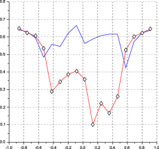
Sample of cross-reference to figure. Figure 1 shows that is not easy to get something on paper.
5 Headings
5.1 Subsection
Carr-Goldstein based their model on balancing methods and biochemical knowledge. The original model (1980) contained an equation for the oxygen dynamics which has been omitted in a second paper (1981). This simplified model shall be discussed here.
5.1.1 Subsubsection
Carr-Goldstein based their model on balancing methods and biochemical knowledge. The original model (1980) contained an equation for the oxygen dynamics which has been omitted in a second paper (1981). This simplified model shall be discussed here.
6 Equations and the like
Two equations:
| (6.1) |
and
| (6.2) |
Two equation arrays:
| (6.3) | |||||
| (6.4) | |||||
| (6.5) | |||||
| (6.6) |
and,
| (6.7) | |||||
| (6.8) | |||||
| (6.9) |
Appendix A Appendix section
We consider a sequence of queueing systems indexed by . It is assumed that each system is composed of stations, indexed by through , and customer classes, indexed by through . Each customer class has a fixed route through the network of stations. Customers in class , , arrive to the system according to a renewal process, independently of the arrivals of the other customer classes. These customers move through the network, never visiting a station more than once, until they eventually exit the system.
A.1 Appendix subsection
However, different customer classes may visit stations in different orders; the system is not necessarily “feed-forward.” We define the path of class customers in as the sequence of servers they encounter along their way through the network and denote it by
| (A.1) |
[Acknowledgments] And this is an acknowledgements section with a heading that was produced by the section* command. Thank you all for helping me writing this LaTeX sample file.
Title of Supplement A \sdescriptionShort description of Supplement A. {supplement} \stitleTitle of Supplement B \sdescriptionShort description of Supplement B.
References
- [1] Billingsley, P. (1999). Convergence of Probability Measures, 2nd ed. Wiley, New York. \MR1700749
- [2] Bourbaki, N. (1966). General Topology 1. Addison–Wesley, Reading, MA.
- [3] Ethier, S. N. and Kurtz, T. G. (1985). Markov Processes: Characterization and Convergence. Wiley, New York. \MR838085
- [4] Prokhorov, Yu. (1956). Convergence of random processes and limit theorems in probability theory. Theory Probab. Appl. 1 157–214. \MR84896