A Search for Neutrino Emission from Fast Radio Bursts with Six Years of IceCube Data

IceCube Collaboration¹¹1: M. G. Aartsen¹¹affiliation: Dept. of Physics and Astronomy, University of Canterbury, Private Bag 4800, Christchurch, New Zealand , M. Ackermann²²affiliation: DESY, D-15738 Zeuthen, Germany , J. Adams¹¹affiliation: Dept. of Physics and Astronomy, University of Canterbury, Private Bag 4800, Christchurch, New Zealand , J. A. Aguilar³³affiliation: Université Libre de Bruxelles, Science Faculty CP230, B-1050 Brussels, Belgium , M. Ahlers⁴⁴affiliation: Niels Bohr Institute, University of Copenhagen, DK-2100 Copenhagen, Denmark , M. Ahrens⁵⁵affiliation: Oskar Klein Centre and Dept. of Physics, Stockholm University, SE-10691 Stockholm, Sweden , I. Al Samarai⁶⁶affiliation: Département de physique nucléaire et corpusculaire, Université de Genève, CH-1211 Genève, Switzerland , D. Altmann⁷⁷affiliation: Erlangen Centre for Astroparticle Physics, Friedrich-Alexander-Universität Erlangen-Nürnberg, D-91058 Erlangen, Germany , K. Andeen⁸⁸affiliation: Department of Physics, Marquette University, Milwaukee, WI, 53201, USA , T. Anderson⁹⁹affiliation: Dept. of Physics, Pennsylvania State University, University Park, PA 16802, USA , I. Ansseau³³affiliation: Université Libre de Bruxelles, Science Faculty CP230, B-1050 Brussels, Belgium , G. Anton⁷⁷affiliation: Erlangen Centre for Astroparticle Physics, Friedrich-Alexander-Universität Erlangen-Nürnberg, D-91058 Erlangen, Germany , C. Argüelles¹⁰¹⁰affiliation: Dept. of Physics, Massachusetts Institute of Technology, Cambridge, MA 02139, USA , J. Auffenberg¹¹¹¹affiliation: III. Physikalisches Institut, RWTH Aachen University, D-52056 Aachen, Germany , S. Axani¹⁰¹⁰affiliation: Dept. of Physics, Massachusetts Institute of Technology, Cambridge, MA 02139, USA , H. Bagherpour¹¹affiliation: Dept. of Physics and Astronomy, University of Canterbury, Private Bag 4800, Christchurch, New Zealand , X. Bai¹²¹²affiliation: Physics Department, South Dakota School of Mines and Technology, Rapid City, SD 57701, USA , J. P. Barron¹³¹³affiliation: Dept. of Physics, University of Alberta, Edmonton, Alberta, Canada T6G 2E1 , S. W. Barwick¹⁴¹⁴affiliation: Dept. of Physics and Astronomy, University of California, Irvine, CA 92697, USA , V. Baum¹⁵¹⁵affiliation: Institute of Physics, University of Mainz, Staudinger Weg 7, D-55099 Mainz, Germany , R. Bay¹⁶¹⁶affiliation: Dept. of Physics, University of California, Berkeley, CA 94720, USA , J. J. Beatty¹⁷¹⁷affiliation: Dept. of Physics and Center for Cosmology and Astro-Particle Physics, Ohio State University, Columbus, OH 43210, USA ¹⁸¹⁸affiliation: Dept. of Astronomy, Ohio State University, Columbus, OH 43210, USA , J. Becker Tjus¹⁹¹⁹affiliation: Fakultät für Physik & Astronomie, Ruhr-Universität Bochum, D-44780 Bochum, Germany , K.-H. Becker²⁰²⁰affiliation: Dept. of Physics, University of Wuppertal, D-42119 Wuppertal, Germany , S. BenZvi²¹²¹affiliation: Dept. of Physics and Astronomy, University of Rochester, Rochester, NY 14627, USA , D. Berley²²²²affiliation: Dept. of Physics, University of Maryland, College Park, MD 20742, USA , E. Bernardini²²affiliation: DESY, D-15738 Zeuthen, Germany , D. Z. Besson²³²³affiliation: Dept. of Physics and Astronomy, University of Kansas, Lawrence, KS 66045, USA , G. Binder²⁴²⁴affiliation: Lawrence Berkeley National Laboratory, Berkeley, CA 94720, USA ¹⁶¹⁶affiliation: Dept. of Physics, University of California, Berkeley, CA 94720, USA , D. Bindig²⁰²⁰affiliation: Dept. of Physics, University of Wuppertal, D-42119 Wuppertal, Germany , E. Blaufuss²²²²affiliation: Dept. of Physics, University of Maryland, College Park, MD 20742, USA , S. Blot²²affiliation: DESY, D-15738 Zeuthen, Germany , C. Bohm⁵⁵affiliation: Oskar Klein Centre and Dept. of Physics, Stockholm University, SE-10691 Stockholm, Sweden , M. Börner²⁵²⁵affiliation: Dept. of Physics, TU Dortmund University, D-44221 Dortmund, Germany , F. Bos¹⁹¹⁹affiliation: Fakultät für Physik & Astronomie, Ruhr-Universität Bochum, D-44780 Bochum, Germany , D. Bose²⁶²⁶affiliation: Dept. of Physics, Sungkyunkwan University, Suwon 440-746, Korea , S. Böser¹⁵¹⁵affiliation: Institute of Physics, University of Mainz, Staudinger Weg 7, D-55099 Mainz, Germany , O. Botner²⁷²⁷affiliation: Dept. of Physics and Astronomy, Uppsala University, Box 516, S-75120 Uppsala, Sweden , E. Bourbeau⁴⁴affiliation: Niels Bohr Institute, University of Copenhagen, DK-2100 Copenhagen, Denmark , J. Bourbeau²⁸²⁸affiliation: Dept. of Physics and Wisconsin IceCube Particle Astrophysics Center, University of Wisconsin, Madison, WI 53706, USA , F. Bradascio²²affiliation: DESY, D-15738 Zeuthen, Germany , J. Braun²⁸²⁸affiliation: Dept. of Physics and Wisconsin IceCube Particle Astrophysics Center, University of Wisconsin, Madison, WI 53706, USA , L. Brayeur²⁹²⁹affiliation: Vrije Universiteit Brussel (VUB), Dienst ELEM, B-1050 Brussels, Belgium , M. Brenzke¹¹¹¹affiliation: III. Physikalisches Institut, RWTH Aachen University, D-52056 Aachen, Germany , H.-P. Bretz²²affiliation: DESY, D-15738 Zeuthen, Germany , S. Bron⁶⁶affiliation: Département de physique nucléaire et corpusculaire, Université de Genève, CH-1211 Genève, Switzerland , J. Brostean-Kaiser²²affiliation: DESY, D-15738 Zeuthen, Germany , A. Burgman²⁷²⁷affiliation: Dept. of Physics and Astronomy, Uppsala University, Box 516, S-75120 Uppsala, Sweden , T. Carver⁶⁶affiliation: Département de physique nucléaire et corpusculaire, Université de Genève, CH-1211 Genève, Switzerland , J. Casey²⁸²⁸affiliation: Dept. of Physics and Wisconsin IceCube Particle Astrophysics Center, University of Wisconsin, Madison, WI 53706, USA , M. Casier²⁹²⁹affiliation: Vrije Universiteit Brussel (VUB), Dienst ELEM, B-1050 Brussels, Belgium , E. Cheung²²²²affiliation: Dept. of Physics, University of Maryland, College Park, MD 20742, USA , D. Chirkin²⁸²⁸affiliation: Dept. of Physics and Wisconsin IceCube Particle Astrophysics Center, University of Wisconsin, Madison, WI 53706, USA , A. Christov⁶⁶affiliation: Département de physique nucléaire et corpusculaire, Université de Genève, CH-1211 Genève, Switzerland , K. Clark³⁰³⁰affiliation: SNOLAB, 1039 Regional Road 24, Creighton Mine 9, Lively, ON, Canada P3Y 1N2 , L. Classen³¹³¹affiliation: Institut für Kernphysik, Westfälische Wilhelms-Universität Münster, D-48149 Münster, Germany , S. Coenders³²³²affiliation: Physik-department, Technische Universität München, D-85748 Garching, Germany , G. H. Collin¹⁰¹⁰affiliation: Dept. of Physics, Massachusetts Institute of Technology, Cambridge, MA 02139, USA , J. M. Conrad¹⁰¹⁰affiliation: Dept. of Physics, Massachusetts Institute of Technology, Cambridge, MA 02139, USA , D. F. Cowen⁹⁹affiliation: Dept. of Physics, Pennsylvania State University, University Park, PA 16802, USA ³³³³affiliation: Dept. of Astronomy and Astrophysics, Pennsylvania State University, University Park, PA 16802, USA , R. Cross²¹²¹affiliation: Dept. of Physics and Astronomy, University of Rochester, Rochester, NY 14627, USA , M. Day²⁸²⁸affiliation: Dept. of Physics and Wisconsin IceCube Particle Astrophysics Center, University of Wisconsin, Madison, WI 53706, USA , J. P. A. M. de André³⁴³⁴affiliation: Dept. of Physics and Astronomy, Michigan State University, East Lansing, MI 48824, USA , C. De Clercq²⁹²⁹affiliation: Vrije Universiteit Brussel (VUB), Dienst ELEM, B-1050 Brussels, Belgium , J. J. DeLaunay⁹⁹affiliation: Dept. of Physics, Pennsylvania State University, University Park, PA 16802, USA , H. Dembinski³⁵³⁵affiliation: Bartol Research Institute and Dept. of Physics and Astronomy, University of Delaware, Newark, DE 19716, USA , S. De Ridder³⁶³⁶affiliation: Dept. of Physics and Astronomy, University of Gent, B-9000 Gent, Belgium , P. Desiati²⁸²⁸affiliation: Dept. of Physics and Wisconsin IceCube Particle Astrophysics Center, University of Wisconsin, Madison, WI 53706, USA , K. D. de Vries²⁹²⁹affiliation: Vrije Universiteit Brussel (VUB), Dienst ELEM, B-1050 Brussels, Belgium , G. de Wasseige²⁹²⁹affiliation: Vrije Universiteit Brussel (VUB), Dienst ELEM, B-1050 Brussels, Belgium , M. de With³⁷³⁷affiliation: Institut für Physik, Humboldt-Universität zu Berlin, D-12489 Berlin, Germany , T. DeYoung³⁴³⁴affiliation: Dept. of Physics and Astronomy, Michigan State University, East Lansing, MI 48824, USA , J. C. Díaz-Vélez²⁸²⁸affiliation: Dept. of Physics and Wisconsin IceCube Particle Astrophysics Center, University of Wisconsin, Madison, WI 53706, USA , V. di Lorenzo¹⁵¹⁵affiliation: Institute of Physics, University of Mainz, Staudinger Weg 7, D-55099 Mainz, Germany , H. Dujmovic²⁶²⁶affiliation: Dept. of Physics, Sungkyunkwan University, Suwon 440-746, Korea , J. P. Dumm⁵⁵affiliation: Oskar Klein Centre and Dept. of Physics, Stockholm University, SE-10691 Stockholm, Sweden , M. Dunkman⁹⁹affiliation: Dept. of Physics, Pennsylvania State University, University Park, PA 16802, USA , E. Dvorak¹²¹²affiliation: Physics Department, South Dakota School of Mines and Technology, Rapid City, SD 57701, USA , B. Eberhardt¹⁵¹⁵affiliation: Institute of Physics, University of Mainz, Staudinger Weg 7, D-55099 Mainz, Germany , T. Ehrhardt¹⁵¹⁵affiliation: Institute of Physics, University of Mainz, Staudinger Weg 7, D-55099 Mainz, Germany , B. Eichmann¹⁹¹⁹affiliation: Fakultät für Physik & Astronomie, Ruhr-Universität Bochum, D-44780 Bochum, Germany , P. Eller⁹⁹affiliation: Dept. of Physics, Pennsylvania State University, University Park, PA 16802, USA , P. A. Evenson³⁵³⁵affiliation: Bartol Research Institute and Dept. of Physics and Astronomy, University of Delaware, Newark, DE 19716, USA , S. Fahey²⁸²⁸affiliation: Dept. of Physics and Wisconsin IceCube Particle Astrophysics Center, University of Wisconsin, Madison, WI 53706, USA , A. R. Fazely³⁸³⁸affiliation: Dept. of Physics, Southern University, Baton Rouge, LA 70813, USA , J. Felde²²²²affiliation: Dept. of Physics, University of Maryland, College Park, MD 20742, USA , K. Filimonov¹⁶¹⁶affiliation: Dept. of Physics, University of California, Berkeley, CA 94720, USA , C. Finley⁵⁵affiliation: Oskar Klein Centre and Dept. of Physics, Stockholm University, SE-10691 Stockholm, Sweden , S. Flis⁵⁵affiliation: Oskar Klein Centre and Dept. of Physics, Stockholm University, SE-10691 Stockholm, Sweden , A. Franckowiak²²affiliation: DESY, D-15738 Zeuthen, Germany , E. Friedman²²²²affiliation: Dept. of Physics, University of Maryland, College Park, MD 20742, USA , T. K. Gaisser³⁵³⁵affiliation: Bartol Research Institute and Dept. of Physics and Astronomy, University of Delaware, Newark, DE 19716, USA , J. Gallagher³⁹³⁹affiliation: Dept. of Astronomy, University of Wisconsin, Madison, WI 53706, USA , L. Gerhardt²⁴²⁴affiliation: Lawrence Berkeley National Laboratory, Berkeley, CA 94720, USA , K. Ghorbani²⁸²⁸affiliation: Dept. of Physics and Wisconsin IceCube Particle Astrophysics Center, University of Wisconsin, Madison, WI 53706, USA , W. Giang¹³¹³affiliation: Dept. of Physics, University of Alberta, Edmonton, Alberta, Canada T6G 2E1 , T. Glauch³²³²affiliation: Physik-department, Technische Universität München, D-85748 Garching, Germany , T. Glüsenkamp⁷⁷affiliation: Erlangen Centre for Astroparticle Physics, Friedrich-Alexander-Universität Erlangen-Nürnberg, D-91058 Erlangen, Germany , A. Goldschmidt²⁴²⁴affiliation: Lawrence Berkeley National Laboratory, Berkeley, CA 94720, USA , J. G. Gonzalez³⁵³⁵affiliation: Bartol Research Institute and Dept. of Physics and Astronomy, University of Delaware, Newark, DE 19716, USA , D. Grant¹³¹³affiliation: Dept. of Physics, University of Alberta, Edmonton, Alberta, Canada T6G 2E1 , Z. Griffith²⁸²⁸affiliation: Dept. of Physics and Wisconsin IceCube Particle Astrophysics Center, University of Wisconsin, Madison, WI 53706, USA , C. Haack¹¹¹¹affiliation: III. Physikalisches Institut, RWTH Aachen University, D-52056 Aachen, Germany , A. Hallgren²⁷²⁷affiliation: Dept. of Physics and Astronomy, Uppsala University, Box 516, S-75120 Uppsala, Sweden , F. Halzen²⁸²⁸affiliation: Dept. of Physics and Wisconsin IceCube Particle Astrophysics Center, University of Wisconsin, Madison, WI 53706, USA , K. Hanson²⁸²⁸affiliation: Dept. of Physics and Wisconsin IceCube Particle Astrophysics Center, University of Wisconsin, Madison, WI 53706, USA , D. Hebecker³⁷³⁷affiliation: Institut für Physik, Humboldt-Universität zu Berlin, D-12489 Berlin, Germany , D. Heereman³³affiliation: Université Libre de Bruxelles, Science Faculty CP230, B-1050 Brussels, Belgium , K. Helbing²⁰²⁰affiliation: Dept. of Physics, University of Wuppertal, D-42119 Wuppertal, Germany , R. Hellauer²²²²affiliation: Dept. of Physics, University of Maryland, College Park, MD 20742, USA , S. Hickford²⁰²⁰affiliation: Dept. of Physics, University of Wuppertal, D-42119 Wuppertal, Germany , J. Hignight³⁴³⁴affiliation: Dept. of Physics and Astronomy, Michigan State University, East Lansing, MI 48824, USA , G. C. Hill⁴⁰⁴⁰affiliation: Department of Physics, University of Adelaide, Adelaide, 5005, Australia , K. D. Hoffman²²²²affiliation: Dept. of Physics, University of Maryland, College Park, MD 20742, USA , R. Hoffmann²⁰²⁰affiliation: Dept. of Physics, University of Wuppertal, D-42119 Wuppertal, Germany , T. Hoinka²⁵²⁵affiliation: Dept. of Physics, TU Dortmund University, D-44221 Dortmund, Germany , B. Hokanson-Fasig²⁸²⁸affiliation: Dept. of Physics and Wisconsin IceCube Particle Astrophysics Center, University of Wisconsin, Madison, WI 53706, USA , K. Hoshina²⁸²⁸affiliation: Dept. of Physics and Wisconsin IceCube Particle Astrophysics Center, University of Wisconsin, Madison, WI 53706, USA ⁵³⁵³affiliation: Earthquake Research Institute, University of Tokyo, Bunkyo, Tokyo 113-0032, Japan , F. Huang⁹⁹affiliation: Dept. of Physics, Pennsylvania State University, University Park, PA 16802, USA , M. Huber³²³²affiliation: Physik-department, Technische Universität München, D-85748 Garching, Germany , K. Hultqvist⁵⁵affiliation: Oskar Klein Centre and Dept. of Physics, Stockholm University, SE-10691 Stockholm, Sweden , M. Hünnefeld²⁵²⁵affiliation: Dept. of Physics, TU Dortmund University, D-44221 Dortmund, Germany , S. In²⁶²⁶affiliation: Dept. of Physics, Sungkyunkwan University, Suwon 440-746, Korea , A. Ishihara⁴¹⁴¹affiliation: Dept. of Physics and Institute for Global Prominent Research, Chiba University, Chiba 263-8522, Japan , E. Jacobi²²affiliation: DESY, D-15738 Zeuthen, Germany , G. S. Japaridze⁴²⁴²affiliation: CTSPS, Clark-Atlanta University, Atlanta, GA 30314, USA , M. Jeong²⁶²⁶affiliation: Dept. of Physics, Sungkyunkwan University, Suwon 440-746, Korea , K. Jero²⁸²⁸affiliation: Dept. of Physics and Wisconsin IceCube Particle Astrophysics Center, University of Wisconsin, Madison, WI 53706, USA , B. J. P. Jones⁴³⁴³affiliation: Dept. of Physics, University of Texas at Arlington, 502 Yates St., Science Hall Rm 108, Box 19059, Arlington, TX 76019, USA , P. Kalaczynski¹¹¹¹affiliation: III. Physikalisches Institut, RWTH Aachen University, D-52056 Aachen, Germany , W. Kang²⁶²⁶affiliation: Dept. of Physics, Sungkyunkwan University, Suwon 440-746, Korea , A. Kappes³¹³¹affiliation: Institut für Kernphysik, Westfälische Wilhelms-Universität Münster, D-48149 Münster, Germany , T. Karg²²affiliation: DESY, D-15738 Zeuthen, Germany , A. Karle²⁸²⁸affiliation: Dept. of Physics and Wisconsin IceCube Particle Astrophysics Center, University of Wisconsin, Madison, WI 53706, USA , U. Katz⁷⁷affiliation: Erlangen Centre for Astroparticle Physics, Friedrich-Alexander-Universität Erlangen-Nürnberg, D-91058 Erlangen, Germany , M. Kauer²⁸²⁸affiliation: Dept. of Physics and Wisconsin IceCube Particle Astrophysics Center, University of Wisconsin, Madison, WI 53706, USA , A. Keivani⁹⁹affiliation: Dept. of Physics, Pennsylvania State University, University Park, PA 16802, USA , J. L. Kelley²⁸²⁸affiliation: Dept. of Physics and Wisconsin IceCube Particle Astrophysics Center, University of Wisconsin, Madison, WI 53706, USA , A. Kheirandish²⁸²⁸affiliation: Dept. of Physics and Wisconsin IceCube Particle Astrophysics Center, University of Wisconsin, Madison, WI 53706, USA , J. Kim²⁶²⁶affiliation: Dept. of Physics, Sungkyunkwan University, Suwon 440-746, Korea , M. Kim⁴¹⁴¹affiliation: Dept. of Physics and Institute for Global Prominent Research, Chiba University, Chiba 263-8522, Japan , T. Kintscher²²affiliation: DESY, D-15738 Zeuthen, Germany , J. Kiryluk⁴⁴⁴⁴affiliation: Dept. of Physics and Astronomy, Stony Brook University, Stony Brook, NY 11794-3800, USA , T. Kittler⁷⁷affiliation: Erlangen Centre for Astroparticle Physics, Friedrich-Alexander-Universität Erlangen-Nürnberg, D-91058 Erlangen, Germany , S. R. Klein²⁴²⁴affiliation: Lawrence Berkeley National Laboratory, Berkeley, CA 94720, USA ¹⁶¹⁶affiliation: Dept. of Physics, University of California, Berkeley, CA 94720, USA , G. Kohnen⁴⁵⁴⁵affiliation: Université de Mons, 7000 Mons, Belgium , R. Koirala³⁵³⁵affiliation: Bartol Research Institute and Dept. of Physics and Astronomy, University of Delaware, Newark, DE 19716, USA , H. Kolanoski³⁷³⁷affiliation: Institut für Physik, Humboldt-Universität zu Berlin, D-12489 Berlin, Germany , L. Köpke¹⁵¹⁵affiliation: Institute of Physics, University of Mainz, Staudinger Weg 7, D-55099 Mainz, Germany , C. Kopper¹³¹³affiliation: Dept. of Physics, University of Alberta, Edmonton, Alberta, Canada T6G 2E1 , S. Kopper⁴⁶⁴⁶affiliation: Dept. of Physics and Astronomy, University of Alabama, Tuscaloosa, AL 35487, USA , J. P. Koschinsky¹¹¹¹affiliation: III. Physikalisches Institut, RWTH Aachen University, D-52056 Aachen, Germany , D. J. Koskinen⁴⁴affiliation: Niels Bohr Institute, University of Copenhagen, DK-2100 Copenhagen, Denmark , M. Kowalski³⁷³⁷affiliation: Institut für Physik, Humboldt-Universität zu Berlin, D-12489 Berlin, Germany ²²affiliation: DESY, D-15738 Zeuthen, Germany , K. Krings³²³²affiliation: Physik-department, Technische Universität München, D-85748 Garching, Germany , M. Kroll¹⁹¹⁹affiliation: Fakultät für Physik & Astronomie, Ruhr-Universität Bochum, D-44780 Bochum, Germany , G. Krückl¹⁵¹⁵affiliation: Institute of Physics, University of Mainz, Staudinger Weg 7, D-55099 Mainz, Germany , J. Kunnen²⁹²⁹affiliation: Vrije Universiteit Brussel (VUB), Dienst ELEM, B-1050 Brussels, Belgium , S. Kunwar²²affiliation: DESY, D-15738 Zeuthen, Germany , N. Kurahashi⁴⁷⁴⁷affiliation: Dept. of Physics, Drexel University, 3141 Chestnut Street, Philadelphia, PA 19104, USA , T. Kuwabara⁴¹⁴¹affiliation: Dept. of Physics and Institute for Global Prominent Research, Chiba University, Chiba 263-8522, Japan , A. Kyriacou⁴⁰⁴⁰affiliation: Department of Physics, University of Adelaide, Adelaide, 5005, Australia , M. Labare³⁶³⁶affiliation: Dept. of Physics and Astronomy, University of Gent, B-9000 Gent, Belgium , J. L. Lanfranchi⁹⁹affiliation: Dept. of Physics, Pennsylvania State University, University Park, PA 16802, USA , M. J. Larson⁴⁴affiliation: Niels Bohr Institute, University of Copenhagen, DK-2100 Copenhagen, Denmark , F. Lauber²⁰²⁰affiliation: Dept. of Physics, University of Wuppertal, D-42119 Wuppertal, Germany , M. Lesiak-Bzdak⁴⁴⁴⁴affiliation: Dept. of Physics and Astronomy, Stony Brook University, Stony Brook, NY 11794-3800, USA , M. Leuermann¹¹¹¹affiliation: III. Physikalisches Institut, RWTH Aachen University, D-52056 Aachen, Germany , Q. R. Liu²⁸²⁸affiliation: Dept. of Physics and Wisconsin IceCube Particle Astrophysics Center, University of Wisconsin, Madison, WI 53706, USA , C. J. Lozano Mariscal³¹³¹affiliation: Institut für Kernphysik, Westfälische Wilhelms-Universität Münster, D-48149 Münster, Germany , L. Lu⁴¹⁴¹affiliation: Dept. of Physics and Institute for Global Prominent Research, Chiba University, Chiba 263-8522, Japan , J. Lünemann²⁹²⁹affiliation: Vrije Universiteit Brussel (VUB), Dienst ELEM, B-1050 Brussels, Belgium , W. Luszczak²⁸²⁸affiliation: Dept. of Physics and Wisconsin IceCube Particle Astrophysics Center, University of Wisconsin, Madison, WI 53706, USA , J. Madsen⁴⁸⁴⁸affiliation: Dept. of Physics, University of Wisconsin, River Falls, WI 54022, USA , G. Maggi²⁹²⁹affiliation: Vrije Universiteit Brussel (VUB), Dienst ELEM, B-1050 Brussels, Belgium , K. B. M. Mahn³⁴³⁴affiliation: Dept. of Physics and Astronomy, Michigan State University, East Lansing, MI 48824, USA , S. Mancina²⁸²⁸affiliation: Dept. of Physics and Wisconsin IceCube Particle Astrophysics Center, University of Wisconsin, Madison, WI 53706, USA , R. Maruyama⁴⁹⁴⁹affiliation: Dept. of Physics, Yale University, New Haven, CT 06520, USA , K. Mase⁴¹⁴¹affiliation: Dept. of Physics and Institute for Global Prominent Research, Chiba University, Chiba 263-8522, Japan , R. Maunu²²²²affiliation: Dept. of Physics, University of Maryland, College Park, MD 20742, USA , F. McNally²⁸²⁸affiliation: Dept. of Physics and Wisconsin IceCube Particle Astrophysics Center, University of Wisconsin, Madison, WI 53706, USA , K. Meagher³³affiliation: Université Libre de Bruxelles, Science Faculty CP230, B-1050 Brussels, Belgium , M. Medici⁴⁴affiliation: Niels Bohr Institute, University of Copenhagen, DK-2100 Copenhagen, Denmark , M. Meier²⁵²⁵affiliation: Dept. of Physics, TU Dortmund University, D-44221 Dortmund, Germany , T. Menne²⁵²⁵affiliation: Dept. of Physics, TU Dortmund University, D-44221 Dortmund, Germany , G. Merino²⁸²⁸affiliation: Dept. of Physics and Wisconsin IceCube Particle Astrophysics Center, University of Wisconsin, Madison, WI 53706, USA , T. Meures³³affiliation: Université Libre de Bruxelles, Science Faculty CP230, B-1050 Brussels, Belgium , S. Miarecki²⁴²⁴affiliation: Lawrence Berkeley National Laboratory, Berkeley, CA 94720, USA ¹⁶¹⁶affiliation: Dept. of Physics, University of California, Berkeley, CA 94720, USA , J. Micallef³⁴³⁴affiliation: Dept. of Physics and Astronomy, Michigan State University, East Lansing, MI 48824, USA , G. Momenté¹⁵¹⁵affiliation: Institute of Physics, University of Mainz, Staudinger Weg 7, D-55099 Mainz, Germany , T. Montaruli⁶⁶affiliation: Département de physique nucléaire et corpusculaire, Université de Genève, CH-1211 Genève, Switzerland , R. W. Moore¹³¹³affiliation: Dept. of Physics, University of Alberta, Edmonton, Alberta, Canada T6G 2E1 , M. Moulai¹⁰¹⁰affiliation: Dept. of Physics, Massachusetts Institute of Technology, Cambridge, MA 02139, USA , R. Nahnhauer²²affiliation: DESY, D-15738 Zeuthen, Germany , P. Nakarmi⁴⁶⁴⁶affiliation: Dept. of Physics and Astronomy, University of Alabama, Tuscaloosa, AL 35487, USA , U. Naumann²⁰²⁰affiliation: Dept. of Physics, University of Wuppertal, D-42119 Wuppertal, Germany , G. Neer³⁴³⁴affiliation: Dept. of Physics and Astronomy, Michigan State University, East Lansing, MI 48824, USA , H. Niederhausen⁴⁴⁴⁴affiliation: Dept. of Physics and Astronomy, Stony Brook University, Stony Brook, NY 11794-3800, USA , S. C. Nowicki¹³¹³affiliation: Dept. of Physics, University of Alberta, Edmonton, Alberta, Canada T6G 2E1 , D. R. Nygren²⁴²⁴affiliation: Lawrence Berkeley National Laboratory, Berkeley, CA 94720, USA , A. Obertacke Pollmann²⁰²⁰affiliation: Dept. of Physics, University of Wuppertal, D-42119 Wuppertal, Germany , A. Olivas²²²²affiliation: Dept. of Physics, University of Maryland, College Park, MD 20742, USA , A. O’Murchadha³³affiliation: Université Libre de Bruxelles, Science Faculty CP230, B-1050 Brussels, Belgium , E. O’Sullivan⁵⁵affiliation: Oskar Klein Centre and Dept. of Physics, Stockholm University, SE-10691 Stockholm, Sweden , T. Palczewski²⁴²⁴affiliation: Lawrence Berkeley National Laboratory, Berkeley, CA 94720, USA ¹⁶¹⁶affiliation: Dept. of Physics, University of California, Berkeley, CA 94720, USA , H. Pandya³⁵³⁵affiliation: Bartol Research Institute and Dept. of Physics and Astronomy, University of Delaware, Newark, DE 19716, USA , D. V. Pankova⁹⁹affiliation: Dept. of Physics, Pennsylvania State University, University Park, PA 16802, USA , P. Peiffer¹⁵¹⁵affiliation: Institute of Physics, University of Mainz, Staudinger Weg 7, D-55099 Mainz, Germany , J. A. Pepper⁴⁶⁴⁶affiliation: Dept. of Physics and Astronomy, University of Alabama, Tuscaloosa, AL 35487, USA , C. Pérez de los Heros²⁷²⁷affiliation: Dept. of Physics and Astronomy, Uppsala University, Box 516, S-75120 Uppsala, Sweden , D. Pieloth²⁵²⁵affiliation: Dept. of Physics, TU Dortmund University, D-44221 Dortmund, Germany , E. Pinat³³affiliation: Université Libre de Bruxelles, Science Faculty CP230, B-1050 Brussels, Belgium , M. Plum⁸⁸affiliation: Department of Physics, Marquette University, Milwaukee, WI, 53201, USA , D. Pranav⁵⁰⁵⁰affiliation: School of Physics and Center for Relativistic Astrophysics, Georgia Institute of Technology, Atlanta, GA 30332, USA , P. B. Price¹⁶¹⁶affiliation: Dept. of Physics, University of California, Berkeley, CA 94720, USA , G. T. Przybylski²⁴²⁴affiliation: Lawrence Berkeley National Laboratory, Berkeley, CA 94720, USA , C. Raab³³affiliation: Université Libre de Bruxelles, Science Faculty CP230, B-1050 Brussels, Belgium , L. Rädel¹¹¹¹affiliation: III. Physikalisches Institut, RWTH Aachen University, D-52056 Aachen, Germany , M. Rameez⁴⁴affiliation: Niels Bohr Institute, University of Copenhagen, DK-2100 Copenhagen, Denmark , K. Rawlins⁵¹⁵¹affiliation: Dept. of Physics and Astronomy, University of Alaska Anchorage, 3211 Providence Dr., Anchorage, AK 99508, USA , I. C. Rea³²³²affiliation: Physik-department, Technische Universität München, D-85748 Garching, Germany , R. Reimann¹¹¹¹affiliation: III. Physikalisches Institut, RWTH Aachen University, D-52056 Aachen, Germany , B. Relethford⁴⁷⁴⁷affiliation: Dept. of Physics, Drexel University, 3141 Chestnut Street, Philadelphia, PA 19104, USA , M. Relich⁴¹⁴¹affiliation: Dept. of Physics and Institute for Global Prominent Research, Chiba University, Chiba 263-8522, Japan , E. Resconi³²³²affiliation: Physik-department, Technische Universität München, D-85748 Garching, Germany , W. Rhode²⁵²⁵affiliation: Dept. of Physics, TU Dortmund University, D-44221 Dortmund, Germany , M. Richman⁴⁷⁴⁷affiliation: Dept. of Physics, Drexel University, 3141 Chestnut Street, Philadelphia, PA 19104, USA , S. Robertson⁴⁰⁴⁰affiliation: Department of Physics, University of Adelaide, Adelaide, 5005, Australia , M. Rongen¹¹¹¹affiliation: III. Physikalisches Institut, RWTH Aachen University, D-52056 Aachen, Germany , C. Rott²⁶²⁶affiliation: Dept. of Physics, Sungkyunkwan University, Suwon 440-746, Korea , T. Ruhe²⁵²⁵affiliation: Dept. of Physics, TU Dortmund University, D-44221 Dortmund, Germany , D. Ryckbosch³⁶³⁶affiliation: Dept. of Physics and Astronomy, University of Gent, B-9000 Gent, Belgium , D. Rysewyk³⁴³⁴affiliation: Dept. of Physics and Astronomy, Michigan State University, East Lansing, MI 48824, USA , T. Sälzer¹¹¹¹affiliation: III. Physikalisches Institut, RWTH Aachen University, D-52056 Aachen, Germany , S. E. Sanchez Herrera¹³¹³affiliation: Dept. of Physics, University of Alberta, Edmonton, Alberta, Canada T6G 2E1 , A. Sandrock²⁵²⁵affiliation: Dept. of Physics, TU Dortmund University, D-44221 Dortmund, Germany , J. Sandroos¹⁵¹⁵affiliation: Institute of Physics, University of Mainz, Staudinger Weg 7, D-55099 Mainz, Germany , M. Santander⁴⁶⁴⁶affiliation: Dept. of Physics and Astronomy, University of Alabama, Tuscaloosa, AL 35487, USA , S. Sarkar⁴⁴affiliation: Niels Bohr Institute, University of Copenhagen, DK-2100 Copenhagen, Denmark ⁵²⁵²affiliation: Dept. of Physics, University of Oxford, 1 Keble Road, Oxford OX1 3NP, UK , S. Sarkar¹³¹³affiliation: Dept. of Physics, University of Alberta, Edmonton, Alberta, Canada T6G 2E1 , K. Satalecka²²affiliation: DESY, D-15738 Zeuthen, Germany , P. Schlunder²⁵²⁵affiliation: Dept. of Physics, TU Dortmund University, D-44221 Dortmund, Germany , T. Schmidt²²²²affiliation: Dept. of Physics, University of Maryland, College Park, MD 20742, USA , A. Schneider²⁸²⁸affiliation: Dept. of Physics and Wisconsin IceCube Particle Astrophysics Center, University of Wisconsin, Madison, WI 53706, USA , S. Schoenen¹¹¹¹affiliation: III. Physikalisches Institut, RWTH Aachen University, D-52056 Aachen, Germany , S. Schöneberg¹⁹¹⁹affiliation: Fakultät für Physik & Astronomie, Ruhr-Universität Bochum, D-44780 Bochum, Germany , L. Schumacher¹¹¹¹affiliation: III. Physikalisches Institut, RWTH Aachen University, D-52056 Aachen, Germany , D. Seckel³⁵³⁵affiliation: Bartol Research Institute and Dept. of Physics and Astronomy, University of Delaware, Newark, DE 19716, USA , S. Seunarine⁴⁸⁴⁸affiliation: Dept. of Physics, University of Wisconsin, River Falls, WI 54022, USA , J. Soedingrekso²⁵²⁵affiliation: Dept. of Physics, TU Dortmund University, D-44221 Dortmund, Germany , D. Soldin³⁵³⁵affiliation: Bartol Research Institute and Dept. of Physics and Astronomy, University of Delaware, Newark, DE 19716, USA , M. Song²²²²affiliation: Dept. of Physics, University of Maryland, College Park, MD 20742, USA , G. M. Spiczak⁴⁸⁴⁸affiliation: Dept. of Physics, University of Wisconsin, River Falls, WI 54022, USA , C. Spiering²²affiliation: DESY, D-15738 Zeuthen, Germany , J. Stachurska²²affiliation: DESY, D-15738 Zeuthen, Germany , M. Stamatikos¹⁷¹⁷affiliation: Dept. of Physics and Center for Cosmology and Astro-Particle Physics, Ohio State University, Columbus, OH 43210, USA , T. Stanev³⁵³⁵affiliation: Bartol Research Institute and Dept. of Physics and Astronomy, University of Delaware, Newark, DE 19716, USA , A. Stasik²²affiliation: DESY, D-15738 Zeuthen, Germany , J. Stettner¹¹¹¹affiliation: III. Physikalisches Institut, RWTH Aachen University, D-52056 Aachen, Germany , A. Steuer¹⁵¹⁵affiliation: Institute of Physics, University of Mainz, Staudinger Weg 7, D-55099 Mainz, Germany , T. Stezelberger²⁴²⁴affiliation: Lawrence Berkeley National Laboratory, Berkeley, CA 94720, USA , R. G. Stokstad²⁴²⁴affiliation: Lawrence Berkeley National Laboratory, Berkeley, CA 94720, USA , A. Stößl⁴¹⁴¹affiliation: Dept. of Physics and Institute for Global Prominent Research, Chiba University, Chiba 263-8522, Japan , N. L. Strotjohann²²affiliation: DESY, D-15738 Zeuthen, Germany , T. Stuttard⁴⁴affiliation: Niels Bohr Institute, University of Copenhagen, DK-2100 Copenhagen, Denmark , G. W. Sullivan²²²²affiliation: Dept. of Physics, University of Maryland, College Park, MD 20742, USA , M. Sutherland¹⁷¹⁷affiliation: Dept. of Physics and Center for Cosmology and Astro-Particle Physics, Ohio State University, Columbus, OH 43210, USA , I. Taboada⁵⁰⁵⁰affiliation: School of Physics and Center for Relativistic Astrophysics, Georgia Institute of Technology, Atlanta, GA 30332, USA , J. Tatar²⁴²⁴affiliation: Lawrence Berkeley National Laboratory, Berkeley, CA 94720, USA ¹⁶¹⁶affiliation: Dept. of Physics, University of California, Berkeley, CA 94720, USA , F. Tenholt¹⁹¹⁹affiliation: Fakultät für Physik & Astronomie, Ruhr-Universität Bochum, D-44780 Bochum, Germany , S. Ter-Antonyan³⁸³⁸affiliation: Dept. of Physics, Southern University, Baton Rouge, LA 70813, USA , A. Terliuk²²affiliation: DESY, D-15738 Zeuthen, Germany , G. Tešić⁹⁹affiliation: Dept. of Physics, Pennsylvania State University, University Park, PA 16802, USA , S. Tilav³⁵³⁵affiliation: Bartol Research Institute and Dept. of Physics and Astronomy, University of Delaware, Newark, DE 19716, USA , P. A. Toale⁴⁶⁴⁶affiliation: Dept. of Physics and Astronomy, University of Alabama, Tuscaloosa, AL 35487, USA , M. N. Tobin²⁸²⁸affiliation: Dept. of Physics and Wisconsin IceCube Particle Astrophysics Center, University of Wisconsin, Madison, WI 53706, USA , S. Toscano²⁹²⁹affiliation: Vrije Universiteit Brussel (VUB), Dienst ELEM, B-1050 Brussels, Belgium , D. Tosi²⁸²⁸affiliation: Dept. of Physics and Wisconsin IceCube Particle Astrophysics Center, University of Wisconsin, Madison, WI 53706, USA , M. Tselengidou⁷⁷affiliation: Erlangen Centre for Astroparticle Physics, Friedrich-Alexander-Universität Erlangen-Nürnberg, D-91058 Erlangen, Germany , C. F. Tung⁵⁰⁵⁰affiliation: School of Physics and Center for Relativistic Astrophysics, Georgia Institute of Technology, Atlanta, GA 30332, USA , A. Turcati³²³²affiliation: Physik-department, Technische Universität München, D-85748 Garching, Germany , C. F. Turley⁹⁹affiliation: Dept. of Physics, Pennsylvania State University, University Park, PA 16802, USA , B. Ty²⁸²⁸affiliation: Dept. of Physics and Wisconsin IceCube Particle Astrophysics Center, University of Wisconsin, Madison, WI 53706, USA , E. Unger²⁷²⁷affiliation: Dept. of Physics and Astronomy, Uppsala University, Box 516, S-75120 Uppsala, Sweden , M. Usner²²affiliation: DESY, D-15738 Zeuthen, Germany , J. Vandenbroucke²⁸²⁸affiliation: Dept. of Physics and Wisconsin IceCube Particle Astrophysics Center, University of Wisconsin, Madison, WI 53706, USA , W. Van Driessche³⁶³⁶affiliation: Dept. of Physics and Astronomy, University of Gent, B-9000 Gent, Belgium , N. van Eijndhoven²⁹²⁹affiliation: Vrije Universiteit Brussel (VUB), Dienst ELEM, B-1050 Brussels, Belgium , S. Vanheule³⁶³⁶affiliation: Dept. of Physics and Astronomy, University of Gent, B-9000 Gent, Belgium , J. van Santen²²affiliation: DESY, D-15738 Zeuthen, Germany , M. Vehring¹¹¹¹affiliation: III. Physikalisches Institut, RWTH Aachen University, D-52056 Aachen, Germany , E. Vogel¹¹¹¹affiliation: III. Physikalisches Institut, RWTH Aachen University, D-52056 Aachen, Germany , M. Vraeghe³⁶³⁶affiliation: Dept. of Physics and Astronomy, University of Gent, B-9000 Gent, Belgium , C. Walck⁵⁵affiliation: Oskar Klein Centre and Dept. of Physics, Stockholm University, SE-10691 Stockholm, Sweden , A. Wallace⁴⁰⁴⁰affiliation: Department of Physics, University of Adelaide, Adelaide, 5005, Australia , M. Wallraff¹¹¹¹affiliation: III. Physikalisches Institut, RWTH Aachen University, D-52056 Aachen, Germany , F. D. Wandler¹³¹³affiliation: Dept. of Physics, University of Alberta, Edmonton, Alberta, Canada T6G 2E1 , N. Wandkowsky²⁸²⁸affiliation: Dept. of Physics and Wisconsin IceCube Particle Astrophysics Center, University of Wisconsin, Madison, WI 53706, USA , A. Waza¹¹¹¹affiliation: III. Physikalisches Institut, RWTH Aachen University, D-52056 Aachen, Germany , C. Weaver¹³¹³affiliation: Dept. of Physics, University of Alberta, Edmonton, Alberta, Canada T6G 2E1 , M. J. Weiss⁹⁹affiliation: Dept. of Physics, Pennsylvania State University, University Park, PA 16802, USA , C. Wendt²⁸²⁸affiliation: Dept. of Physics and Wisconsin IceCube Particle Astrophysics Center, University of Wisconsin, Madison, WI 53706, USA , J. Werthebach²⁵²⁵affiliation: Dept. of Physics, TU Dortmund University, D-44221 Dortmund, Germany , S. Westerhoff²⁸²⁸affiliation: Dept. of Physics and Wisconsin IceCube Particle Astrophysics Center, University of Wisconsin, Madison, WI 53706, USA , B. J. Whelan⁴⁰⁴⁰affiliation: Department of Physics, University of Adelaide, Adelaide, 5005, Australia , K. Wiebe¹⁵¹⁵affiliation: Institute of Physics, University of Mainz, Staudinger Weg 7, D-55099 Mainz, Germany , C. H. Wiebusch¹¹¹¹affiliation: III. Physikalisches Institut, RWTH Aachen University, D-52056 Aachen, Germany , L. Wille²⁸²⁸affiliation: Dept. of Physics and Wisconsin IceCube Particle Astrophysics Center, University of Wisconsin, Madison, WI 53706, USA , D. R. Williams⁴⁶⁴⁶affiliation: Dept. of Physics and Astronomy, University of Alabama, Tuscaloosa, AL 35487, USA , L. Wills⁴⁷⁴⁷affiliation: Dept. of Physics, Drexel University, 3141 Chestnut Street, Philadelphia, PA 19104, USA , M. Wolf²⁸²⁸affiliation: Dept. of Physics and Wisconsin IceCube Particle Astrophysics Center, University of Wisconsin, Madison, WI 53706, USA , J. Wood²⁸²⁸affiliation: Dept. of Physics and Wisconsin IceCube Particle Astrophysics Center, University of Wisconsin, Madison, WI 53706, USA , T. R. Wood¹³¹³affiliation: Dept. of Physics, University of Alberta, Edmonton, Alberta, Canada T6G 2E1 , E. Woolsey¹³¹³affiliation: Dept. of Physics, University of Alberta, Edmonton, Alberta, Canada T6G 2E1 , K. Woschnagg¹⁶¹⁶affiliation: Dept. of Physics, University of California, Berkeley, CA 94720, USA , D. L. Xu²⁸²⁸affiliation: Dept. of Physics and Wisconsin IceCube Particle Astrophysics Center, University of Wisconsin, Madison, WI 53706, USA , X. W. Xu³⁸³⁸affiliation: Dept. of Physics, Southern University, Baton Rouge, LA 70813, USA , Y. Xu⁴⁴⁴⁴affiliation: Dept. of Physics and Astronomy, Stony Brook University, Stony Brook, NY 11794-3800, USA , J. P. Yanez¹³¹³affiliation: Dept. of Physics, University of Alberta, Edmonton, Alberta, Canada T6G 2E1 , G. Yodh¹⁴¹⁴affiliation: Dept. of Physics and Astronomy, University of California, Irvine, CA 92697, USA , S. Yoshida⁴¹⁴¹affiliation: Dept. of Physics and Institute for Global Prominent Research, Chiba University, Chiba 263-8522, Japan , T. Yuan²⁸²⁸affiliation: Dept. of Physics and Wisconsin IceCube Particle Astrophysics Center, University of Wisconsin, Madison, WI 53706, USA , and M. Zoll⁵⁵affiliation: Oskar Klein Centre and Dept. of Physics, Stockholm University, SE-10691 Stockholm, Sweden analysis@icecube.wisc.edu

Abstract

We present a search for coincidence between IceCube TeV neutrinos and fast radio bursts (FRBs). During the search period from 2010 May 31 to 2016 May 12, a total of 29 FRBs with 13 unique locations have been detected in the whole sky. An unbinned maximum likelihood method was used to search for spatial and temporal coincidence between neutrinos and FRBs in expanding time windows, in both the northern and southern hemispheres. No significant correlation was found in six years of IceCube data. Therefore, we set upper limits on neutrino fluence emitted by FRBs as a function of time window duration. We set the most stringent limit obtained to date on neutrino fluence from FRBs with an $E^{-2}$ energy spectrum assumed, which is 0.0021 GeV cm^-2 per burst for emission timescales up to ~10² seconds from the northern hemisphere stacking search.

Fast Radio Bursts — Astrophysical Neutrinos — IceCube

1 Introduction

Fast radio bursts (FRBs) are a new class of astrophysical phenomenon characterized by bright broadband radio emission lasting only a few milliseconds. Since the first FRB discovered in 2007 in archival data from the Parkes Radio Telescope (Lorimer et al., 2007), more than 20 FRBs have been detected by a total of five observatories (Spitler et al., 2014; Masui et al., 2015; Caleb et al., 2017; Bannister et al., 2017). This rules out the hypothesis of instrumental or terrestrial origin of these phenomena. The number of FRBs detected together with the duration and solid angle searched imply an all-sky FRB occurrence rate of a few thousand per day (Thornton et al., 2013; Spitler et al., 2014), which is consistent with 10% of the supernova rate (Murase et al., 2016). The burst durations suggest that FRB progenitors are very compact, with light-transit distances on the order of hundreds of kilometers. The dispersion measures – the time delay of lower frequency signal components, which is proportional to the column density of free electrons along the line of sight – of the detected FRBs are significantly greater than the Milky Way alone could provide (Cordes et al., 2016), and the majority of sources have been detected at high Galactic latitudes, indicating extragalactic origin. The distances of the FRBs extracted from their dispersion measures, however, are only upper limits and precise measurements are yet to be determined, most likely from multi-wavelength observations.

The nature of FRBs is still under heated debate, and a multitude of models have been proposed for the FRB progenitors, the majority of which involve strong magnetic fields and leptonic acceleration. Some models predict millisecond radio bursts from cataclysmic events such as dying stars (Falcke & Rezzolla, 2014), neutron star mergers (Totani, 2013), or evaporating black holes (Rees, 1977). In 2015, 16 additional bursts were detected from the direction of FRB 121102 (Spitler et al., 2014; Scholz et al., 2016), spaced out non-periodically by timescales ranging from seconds to days. This indicates that the cataclysmic scenario is not true at least for this repeating FRB. A multi-wavelength follow-up campaign identified this FRB’s host dwarf galaxy at a distance of ~1 Gpc (Chatterjee et al., 2017). It is unclear whether FRB 121102 is representative of FRBs as a source class or if repetitions are possible for only a subclass of FRBs.

While leptonic acceleration is typically the default assumption for FRB emission in most models, hadronic acceleration is also possible in the associated regions of the progenitors, which would lead to production of high-energy cosmic rays and neutrinos (Li et al., 2014). It has been proposed that cosmological FRBs could link to exotic phenomena such as oscillations of superconducting cosmic strings (Ye et al., 2017), and some authors predict that such cosmic strings could also produce ultra-high energy cosmic rays and neutrinos, from super heavy particle decays (Berezinsky et al., 2009; Lunardini & Sabancilar, 2012). Therefore, both multi-wavelength and multi-messenger follow-ups can provide crucial information to help decipher the origin of FRBs. Here, the IceCube telescope offers the opportunity to search for neutrinos correlated with FRBs.

The IceCube Neutrino Observatory consists of 5160 digital optical modules (DOMs) instrumenting one cubic kilometer of Antarctic ice from depths of 1450 m to 2450 m at the geographic South Pole (Aartsen et al. (2017e), IceCube Collaboration). Charged products of neutrino interactions in the ice create Cherenkov photons which are observed by the DOMs and allow the reconstruction of the initial neutrino energy, direction, and interaction type. Charged-current muon neutrino interactions create muons, which travel along straight paths in the ice, resulting in events with directional resolution $\lesssim 1^{\circ}$ at energies above 1 TeV (Maunu, 2016). The detector – fully installed since 2010 – collects data from the whole sky with an up-time higher than 99% per year, enabling real-time alerts to other instruments and analysis of archival data as a follow-up to interesting signals detected by other observatories.

IceCube has discovered a diffuse astrophysical neutrino flux in the TeV to PeV energy range (Aartsen et al. (2013b), IceCube Collaboration; Aartsen et al. (2013a), IceCube Collaboration; Aartsen et al. (2014), IceCube Collaboration; Aartsen et al. (2015a), IceCube Collaboration; Aartsen et al. (2015c), IceCube Collaboration; Aartsen et al. (2016a), IceCube Collaboration). The arrival directions of these neutrinos are consistent with an isotropic distribution, indicating a majority of them have originated from extragalactic sources. Although tau neutrinos are yet to be identified among the observed flux (Aartsen et al. (2016b), IceCube Collaboration), the flavor ratio is found to be consistent with $\nu_{e}$ : $\nu_{\mu}$ : $\nu_{\tau}$ = 1 : 1 : 1 from analyses which combined multiple data sets (Aartsen et al. (2015b), IceCube Collaboration) and with events starting inside the detector for all flavor channels. (Aartsen et al. (2015d), IceCube Collaboration; Aartsen et al. (2017d), IceCube Collaboration). Close-to-equal flavor ratio is another feature of astrophysical neutrinos which have traversed astronomical distances and hence have reached full mixing (Argüelles et al., 2015; Bustamante et al., 2015). While the astrophysical neutrino flux has been detected in multiple channels with high significance, neither clustering in space or time nor cross correlations to catalogs have been found (Aartsen et al. (2017a), IceCube Collaboration). The once promising sources for high-energy neutrinos such as gamma ray bursts (Abbasi et al. (2012), IceCube Collaboration; Aartsen et al. (2015e), IceCube Collaboration; Aartsen et al. (2017b), IceCube Collaboration) and blazars (Aartsen et al. (2017c), IceCube Collaboration) have been disfavored as the major contributors to the observed flux. To date, the origin of the astrophysical neutrinos remains a mystery.

In Fahey et al. (2017), an analysis of four FRBs with one year of IceCube data was reported. Here we present the results of a more sophisticated study in search of high-energy neutrinos from 29 FRBs using the IceCube Neutrino Observatory. The paper is structured as follows: Section 2 describes the event sample used. We then discuss the analysis method, search strategies and background modeling in Section 3. In Section 4, we present the sensitivities and discovery potentials based on the analysis method and search strategies established in Section 3. We then report the final results and their interpretation in Section 5. Finally, we conclude and discuss the future prospects for FRB follow-ups with IceCube in Section 6.

2 Event Sample

The data used in this analysis are assembled from muon neutrino candidate events selected in previous analyses in search of prompt neutrino coincidence with gamma ray bursts (GRBs) (Aartsen et al. (2015e), IceCube Collaboration; Aartsen et al. (2017b), IceCube Collaboration). It consists of ten data sets: five years of data from the northern hemisphere and five from the southern hemisphere (Table 1). Due to the effects of atmospheric muon contamination, which are strong in the south and negligible in the north, the data samples are constructed in two “hemispheres” separated at a declination of $\delta=-5^{\circ}$ . The northern selection extends to $-5^{\circ}$ rather than $0^{\circ}$ declination because there is still sufficient Earth overburden at $-5^{\circ}$ for efficient absorption of atmospheric muons.

Table 1: For IceCube data during which an FRB was detected, the event rates, numbers of events, and respective livetimes are shown. Here, "IC79" indicates the first year of data used in this analysis, when the IceCube array consisted of 79 strings; "IC86-1", "IC86-2", etc. denote subsequent years of data from the completed 86-string array. The median angular uncertainty among events in each sample is given as a 90% containment radius, assuming each event reconstruction to have a 2-D Gaussian point-spread function. Since the event reconstruction becomes more accurate for higher energy events, the southern data sets have smaller median angular uncertainties as a consequence of harder energy cuts to reduce atmospheric background. Year-to-year variations in event rate and

\sigma_{90\%}

are the result of event selection methods aimed to maximize sensitivity independently for each data set’s corresponding set of sources in a previous search for GRBs, as described in Section 2.

Northern ( $\delta>-5^{\circ}$ ) Data	Start date	End date	Rate (mHz)	Events	Livetime (days)	$\sigma_{90\%}$
IC86-1	2011-05-13	2012-05-15	3.65	107,612	341.9	2.13^∘
IC86-2	2012-05-15	2013-05-02	5.50	157,754	332.2	2.68^∘
IC86-3	2013-05-02	2014-05-06	6.20	193,320	362.2	2.79^∘
IC86-4	2014-05-06	2015-05-15	6.17	197,311	369.8	2.79^∘
IC86-5	2015-05-15	2016-05-12	6.07	186,600	356.8	2.83^∘
Southern ( $\delta<-5^{\circ}$ ) Data	Start date	End date	Rate (mHz)	Events	Livetime (days)	$\sigma_{90\%}$
IC79	2010-05-31	2011-05-13	2.46	67,474	314.6	1.02^∘
IC86-1	2011-05-13	2012-05-15	1.90	58,982	359.6	1.10^∘
IC86-2	2012-05-15	2013-05-02	3.18	91,485	328.6	1.05^∘
IC86-3	2013-05-02	2014-05-06	3.23	100,820	358.6	1.04^∘
IC86-4	2014-05-06	2015-05-18	1.90	60,500	350.7	1.04^∘

2.1 Northern data set

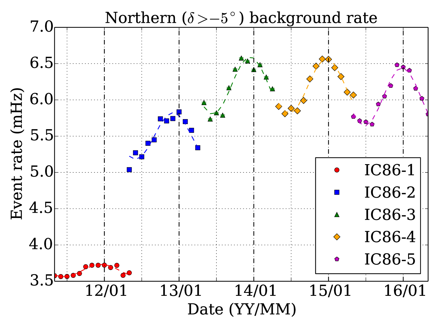
The northern data samples ( $\delta>-5^{\circ}$ ) cover five years of IceCube operation from 2011 May 13 to 2016 May 12, during which 20 northern FRBs were detected (Table 2): three each from a unique source and 17 bursts from FRB 121102. In the northern hemisphere, the Earth filters out cosmic ray-induced atmospheric muons, so the data samples consist primarily of atmospheric muon neutrinos with a median energy on the order of 1 TeV. The event rate in the northern hemisphere increases from 3.5 mHz in the first year (Aartsen et al. (2015e), IceCube Collaboration) to 6 mHz in later years (Aartsen et al. (2017b), IceCube Collaboration), as shown in Figure 1. This year-to-year variation is due largely to two combined effects: first, the initial event selections treat each year of the IceCube data sample independently due to filter and data processing scheme updates in the early years of IceCube operation; second, each data sample was separately optimized for sensitivity to its corresponding set of GRBs¹¹1In the northern data set, the IC86-1 sample was optimized for sensitivity to a stacking search for GRBs. In later years, sensitivity to a max-burst search was instead optimized, accounting for the large year-to-year rate fluctuation between samples IC86-1 and IC86-2 (see Figure 1, Table 1)..

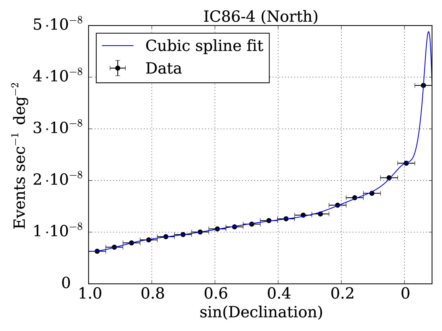
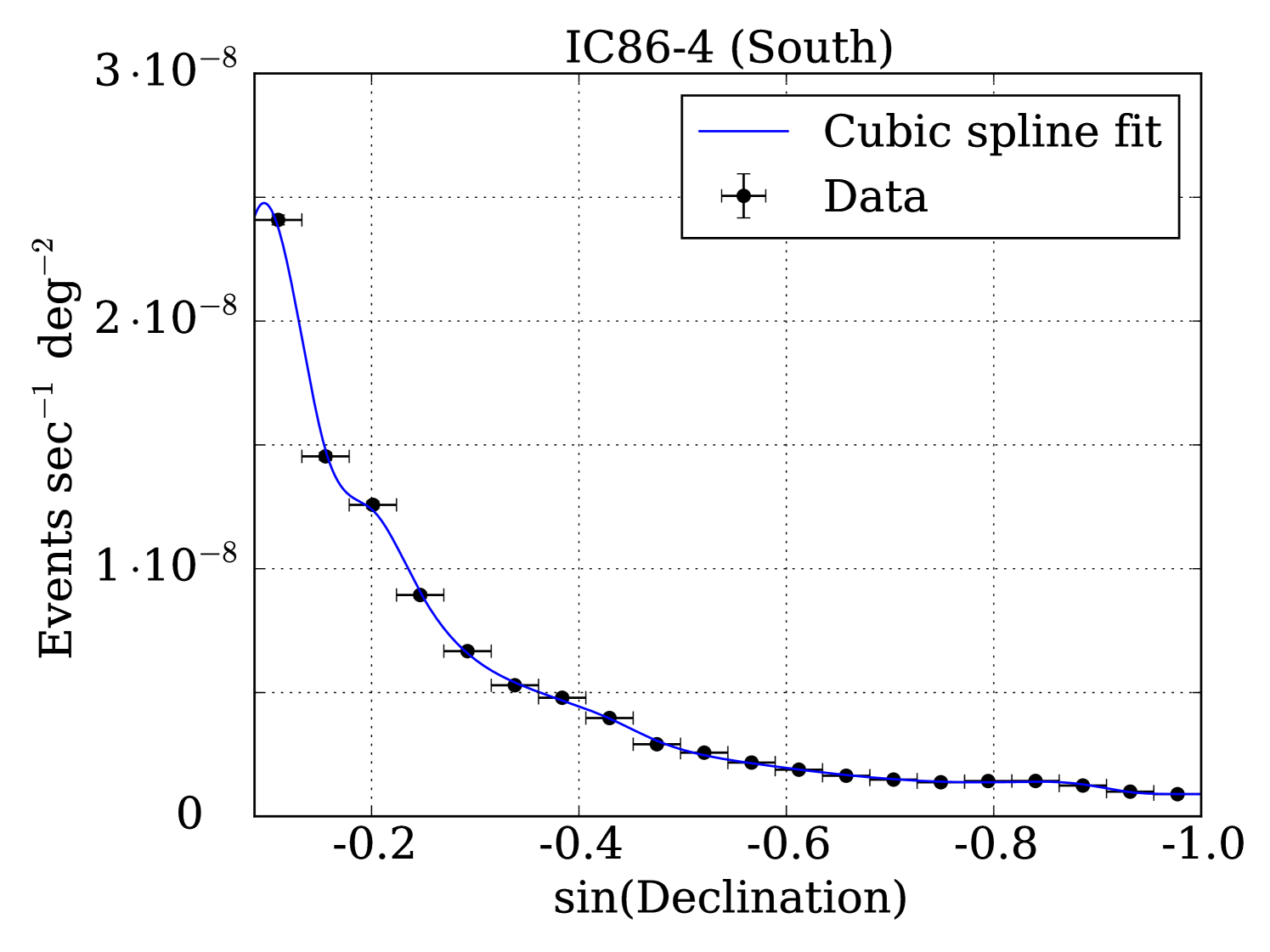
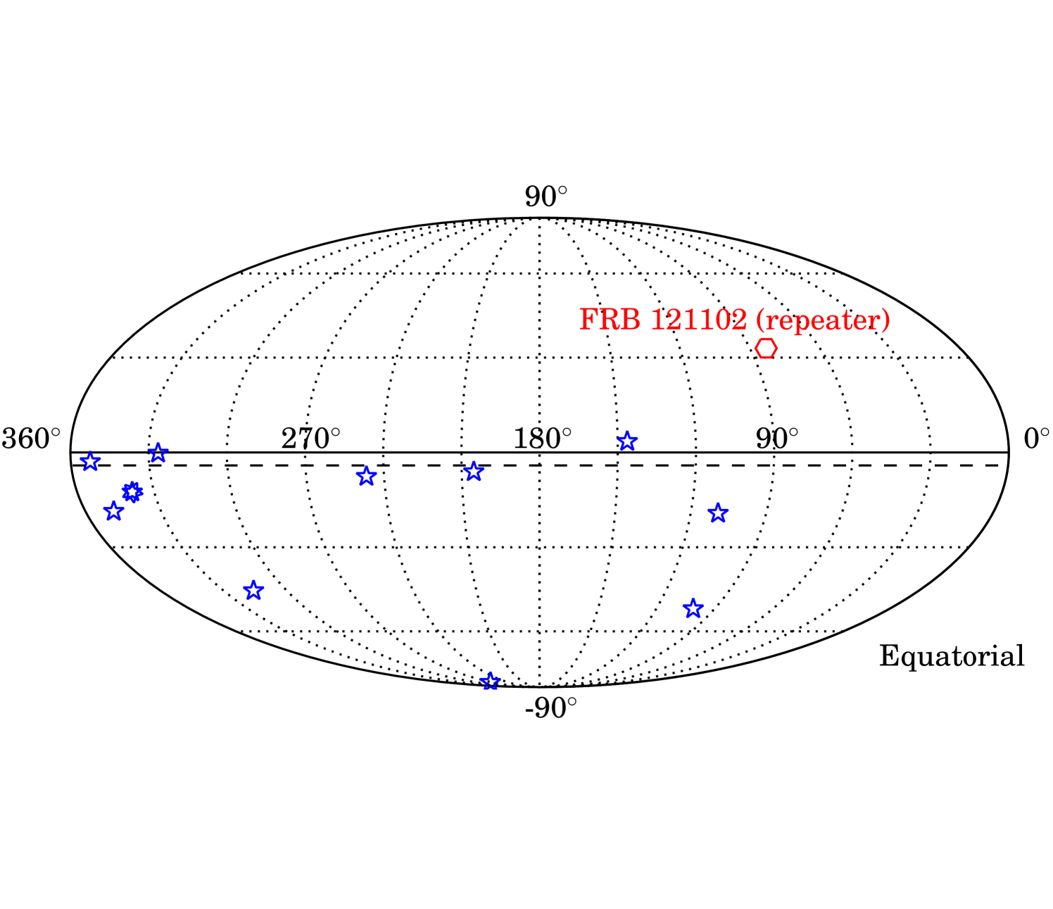
Within each year, a seasonal variation of the background rate can also be seen (Aartsen et al. (2013c), IceCube Collaboration). In the Austral summer, the warming atmosphere expands and increases the average height and mean free path of products from cosmic-ray interactions, allowing pions to more frequently decay into $\mu+\nu_{\mu}$ ²²2IceCube cannot differentiate between neutrinos and anti-neutrinos, so here $\nu_{\mu}$ denotes both neutrinos and anti-neutrinos and increasing the overall rate of atmospheric muons and neutrinos in IceCube. The phase of the seasonal variation in the northern sample is the same as that in the southern sample because the northern sample is dominated by events between $+15^{\circ}$ and $-5^{\circ}$ in declination (Figure 2), which corresponds to production in the atmosphere at latitudes between $-60^{\circ}$ and $-90^{\circ}$ .

2.2 Southern data set

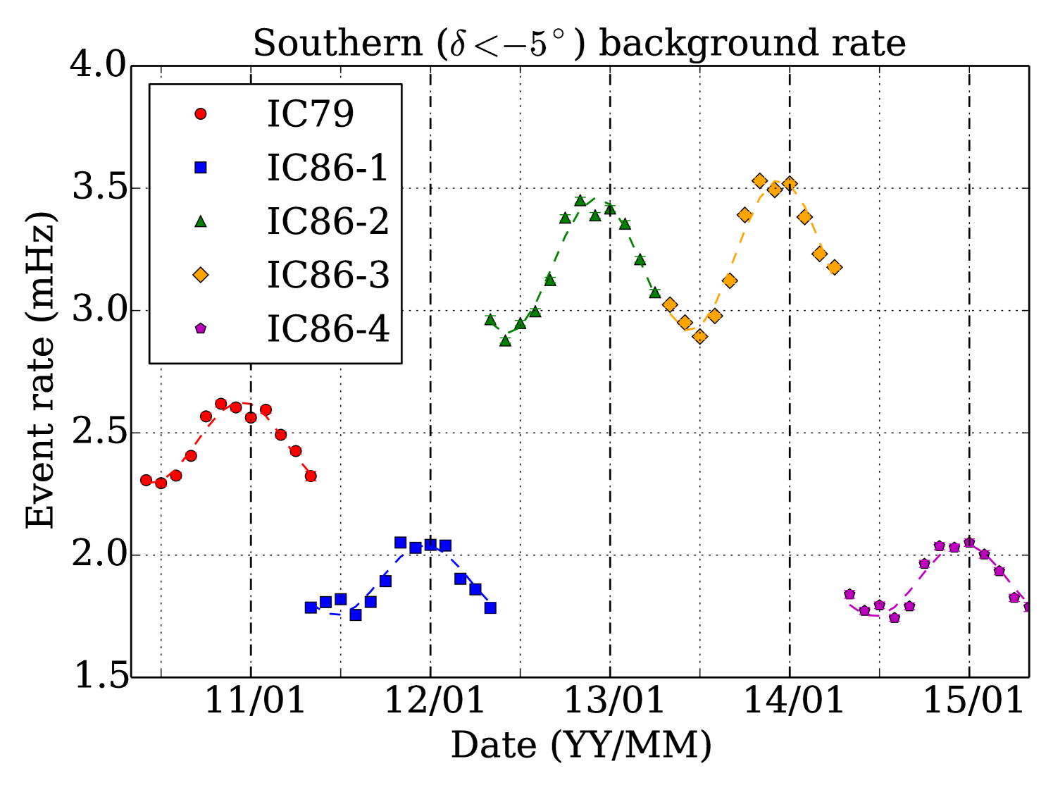
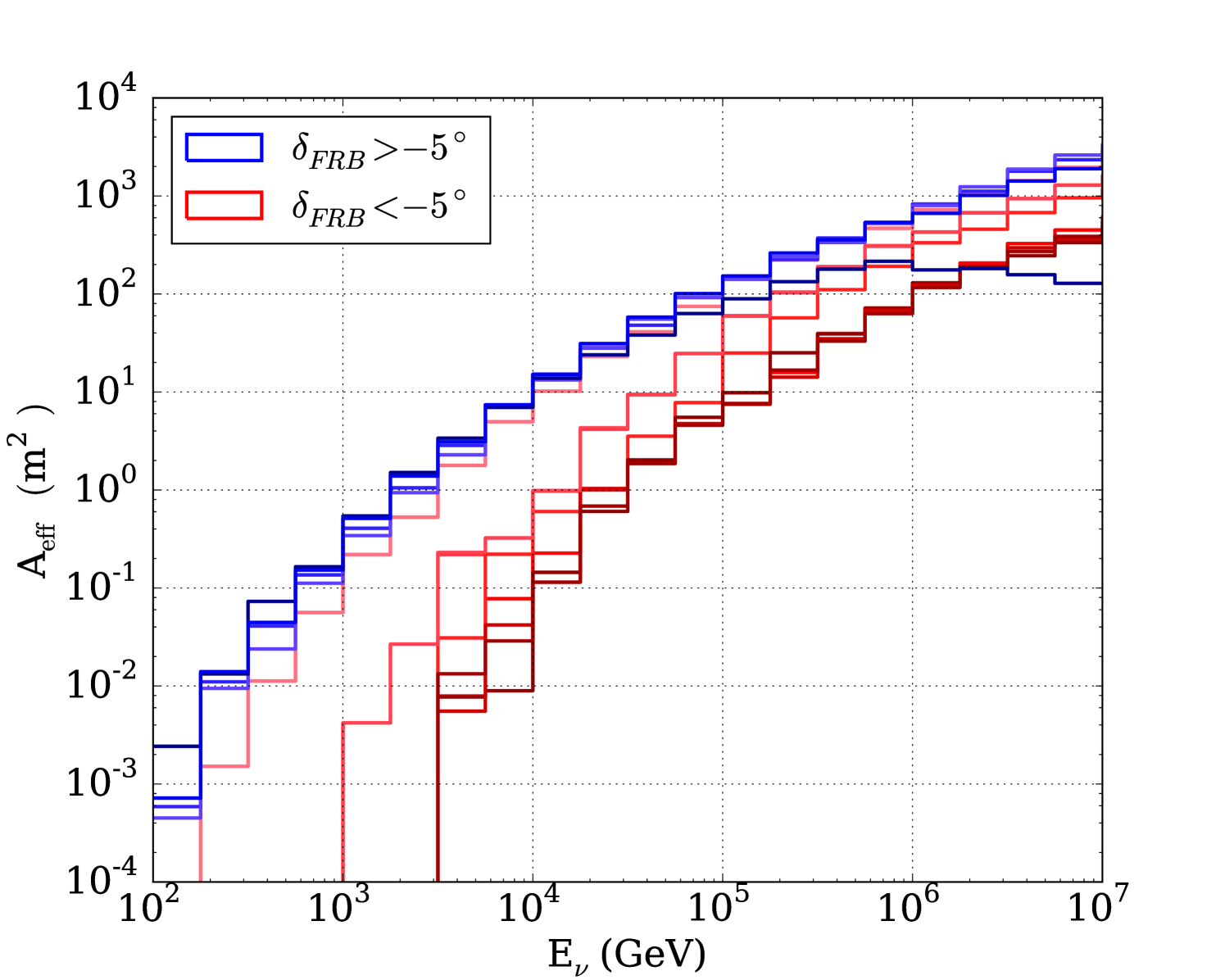
The southern data samples ( $\delta<-5^{\circ}$ ) consist of five years of data from 2010 May 31 to 2015 May 18, during which nine southern FRBs were detected. The year-to-year event rate, 2-3.5 mHz, is lower than that of the northern samples due mainly to a higher energy threshold imposed to reduce background from atmospheric muons and the asymmetric separation of hemispheres which makes the northern hemisphere ~20% larger in solid angle than the southern (Aartsen et al. (2017b), IceCube Collaboration). The southern samples are dominated by down-going atmospheric muons with median energy on the order of 10 TeV. The effective area of IceCube to neutrino events which pass the event selection can be seen in Figure 3, where the effective area has been determined for the declination of each FRB in this analysis.

Refer to caption — Figure 1: Event rates are shown for each data sample, binned by month and fit yearly with one period of a sine function. Year-to-year rate fluctuations reflect changes in event selection methods, not physical changes to the detector, while seasonal variation within each year is the result of the temperature dependence of atmospheric properties which affect atmospheric muon rates. In the northern hemisphere, seasonal variation accounts for a 2-5% amplitude (mean-to-peak) variation in the year-averaged rate. In the southern hemisphere, the amplitude of this fluctuation is 7-10%.

Table 2: 29 FRBs are included in this search: in the north, 20 bursts from 4 unique source locations, and in the south, 9 bursts each with a unique location. For each FRB, arrival time and dispersion-measure-corrected burst duration are provided with RA and Dec (J2000), as well as the IceCube data sample being recorded during its detection. For FRB 121102, which has been found to repeat, we label individual bursts with "b0", "b1", etc., sorted chronologically by time of detection. FRB 121002 was detected as two bursts separated by ~1 ms. It is treated as a single burst in this analysis, but we give both burst durations for completeness.

Northern ( $\delta>-5^{\circ}$ ) FRBs	Time (UTC)	Duration (ms)	RA	Dec	IceCube Data Sample
FRB 110523	2011-05-23 15:06:19.738	1.73	21h 45^′	-00^∘ 12^′	IC86-1
FRB 110703	2011-07-03 18:59:40.591	$<4.3$	23h 30^′	-02^∘ 52^′	IC86-1
FRB 121102 b0	2012-11-02 06:47:17.117	3.3	05h 32^′	33^∘ 05^′	IC86-2
FRB 130628	2013-06-28 03:58:00.02	$<0.05$	09h 03^′	03^∘ 26^′	IC86-3
FRB 121102 b1	2015-05-17 17:42:08.712	3.8	05h 32^′	33^∘ 05^′	IC86-4
FRB 121102 b2	2015-05-17 17:51:40.921	3.3	05h 32^′	33^∘ 05^′	IC86-4
FRB 121102 b3	2015-06-02 16:38:07.575	4.6	05h 32^′	33^∘ 05^′	IC86-5
FRB 121102 b4	2015-06-02 16:47:36.484	8.7	05h 32^′	33^∘ 05^′	IC86-5
FRB 121102 b5	2015-06-02 17:49:18.627	2.8	05h 32^′	33^∘ 05^′	IC86-5
FRB 121102 b6	2015-06-02 17:49:41.319	6.1	05h 32^′	33^∘ 05^′	IC86-5
FRB 121102 b7	2015-06-02 17:50:39.298	6.6	05h 32^′	33^∘ 05^′	IC86-5
FRB 121102 b8	2015-06-02 17:53:45.528	6.0	05h 32^′	33^∘ 05^′	IC86-5
FRB 121102 b9	2015-06-02 17:56:34.787	8.0	05h 32^′	33^∘ 05^′	IC86-5
FRB 121102 b10	2015-06-02 17:57:32.020	3.1	05h 32^′	33^∘ 05^′	IC86-5
FRB 121102 b11	2015-11-13 08:32:42.375	6.73	05h 32^′	33^∘ 05^′	IC86-5
FRB 121102 b12	2015-11-19 10:44:40.524	6.10	05h 32^′	33^∘ 05^′	IC86-5
FRB 121102 b13	2015-11-19 10:51:34.957	6.14	05h 32^′	33^∘ 05^′	IC86-5
FRB 121102 b14	2015-11-19 10:58:56.234	4.30	05h 32^′	33^∘ 05^′	IC86-5
FRB 121102 b15	2015-11-19 11:05:52.492	5.97	05h 32^′	33^∘ 05^′	IC86-5
FRB 121102 b16	2015-12-08 04:54:40.262	2.50	05h 32^′	33^∘ 05^′	IC86-5
Southern ( $\delta<-5^{\circ}$ ) FRBs	Time (UTC)	Duration (ms)	RA	Dec	IceCube Data Sample
FRB 110220	2011-02-20 01:55:48.957	5.6	22h 34^′	-12^∘ 24^′	IC79
FRB 110627	2011-06-27 21:33:17.474	$<1.4$	21h 03^′	-44^∘ 44^′	IC86-1
FRB 120127	2012-01-27 08:11:21.723	$<1.1$	23h 15^′	-18^∘ 25^′	IC86-1
FRB 121002	2012-10-02 13:09:18.402	2.1; 3.7	18h 14^′	-85^∘ 11^′	IC86-2
FRB 130626	2013-06-26 14:56:00.06	$<0.12$	16h 27^′	-07^∘ 27^′	IC86-3
FRB 130729	2013-07-29 09:01:52.64	$<4$	13h 41^′	-05^∘ 59^′	IC86-3
FRB 131104	2013-11-04 18:04:01.2	$<0.64$	06h 44^′	-51^∘ 17^′	IC86-3
FRB 140514	2014-05-14 17:14:11.06	2.8	22h 34^′	-12^∘ 18^′	IC86-4
FRB 150418	2015-04-18 04:29:05.370	0.8	07h 16^′	-19^∘ 00^′	IC86-4

3 Analysis Methods

3.1 Unbinned likelihood method

An unbinned maximum likelihood method is used to search for spatial and temporal coincidence of neutrino events with detected FRBs (Aartsen et al. (2015f), IceCube Collaboration). In a given coincidence window $\Delta$ T centered on the time of detection of each FRB, the likelihood of observing $N$ events for an expected $(n_{s}+n_{b})$ events is

\mathscr{L}(N,\{x_{i}\};n_{s}+n_{b})=\frac{(n_{s}+n_{b})^{N}}{N!}\cdot\exp{[-(n_{s}+n_{b})]}\cdot\prod_{i=1}^{N}\frac{n_{s}S(x_{i})+n_{b}B(x_{i})}{n_{s}+n_{b}}

(1)

where $n_{s}$ and $n_{b}$ are the expected number of observed signal and background events, $x_{i}$ is the reconstructed direction and estimated angular uncertainty for each event $i$ , $S(x_{i})$ is the signal PDF – taken to be a radially symmetric 2D Gaussian with standard deviation $\sigma_{i}$ – evaluated for the angular separation between event $i$ and the FRB with which it is temporally coincident, and $B(x_{i})$ is the background PDF for the data sample to which event $i$ belongs evaluated at the declination of event $i$ . The uncertainties of the FRB locations are taken into account in $S(x_{i})$ , but they are significantly smaller than the median angular uncertainty of the data. In any time window $\Delta$ T, the $N$ events are those which IceCube detected within $\pm\Delta$ T $/2$ of any FRB detection. Before background event rates and PDFs were calculated, on-time data – data collected within $\pm 2$ days of any FRB detection – were removed from the samples until all analysis procedures were determined. The remaining data (>1700 days of data per hemisphere) are considered off-time data, which we used to determine background characteristics to prevent artificial bias from affecting the results of our search. Figure 2 shows examples of off-time data distributions for both northern and southern hemispheres.

A generic test statistic (TS) is used in this analysis, defined as the logarithmic ratio of the likelihood of the alternative hypothesis $\mathscr{L}(N,\{x_{i}\};n_{s}+n_{b})$ and that of the null hypothesis $\mathscr{L}_{0}(N,\{x_{i}\};n_{b})$ , which can be written as

\textrm{TS}=-{n_{s}}+\sum_{i=1}^{N}\ln\Big{[}1+\frac{{n_{s}}S(x_{i})}{n_{b}B(x_{i})}\Big{]}

(2)

The TS is maximized with respect to ${n_{s}}$ to find the most probable number of signal-like events among $N$ temporally coincident events. $n_{b}$ is calculated by multiplying time-dependent background rate for each FRB, modeled from off-time data, by $\Delta$ T.

Two search strategies are implemented based on this test statistic. The stacking search tests the hypothesis that the astrophysical class of FRBs emits neutrinos. In this search, $n_{s}$ and $n_{b}$ are the total number of expected signal and background events contained in the time windows of an entire list of FRBs for the hemisphere. One TS value (with its corresponding $n_{s}$ ) is returned for an ensemble of $N$ events which consist of on-time events from all the bursts. This TS represents the significance of correlation between the events analyzed and the source class as a whole. The max-burst search tests the hypothesis that one or a few bright sources emit neutrinos regardless of source classification. In this search, $n_{s}$ and $n_{b}$ are evaluated separately for each FRB. A TS- $n_{s}$ pair is calculated for each FRB considering only the events coincident with its time window. The most statistically significant of these TS (and its corresponding $n_{s}$ ) is returned as the max-burst TS value of the ensemble.

Since neutrino emission mechanisms and potential neutrino arrival times relative to the time of radio detection are unknown, we employ a model-independent search using an expanding time window, similar to a previous search for prompt neutrino emission from gamma ray bursts by IceCube which found no correlation (Abbasi et al. (2012), IceCube Collaboration). Starting with ${\Delta\textrm{T}=0.01~\textrm{s}}$ centered on each FRB, we search a series of time windows expanding by factors of two, i.e. ${\Delta\textrm{T}=2^{j}\cdot(0.01~\textrm{s})}$ for ${j=0,1,2,...,24}$ . We stop expanding at a time window size of 1.94 days (167772.16 s), where the background becomes significant. For the repeating burst FRB 121102 with burst separations less than the largest time window searched, time windows of consecutive bursts stop expanding when otherwise they would overlap.

In the northern max-burst search, a bright radio burst with a flux of 7.5 Jy detected by the LOFAR radio array (Stewart et al., 2016) was included. This LOFAR burst was detected on 2011 December 24 at 04:33 UTC, near the North Celestial Pole (RA = 22^h53^m47.1^s, DEC = +86^∘21 $\arcmin$ 46.4 $\arcsec$ ) and lasted ~11 minutes. The burst was not consistent with an FRB, so it was not included in the stacking search, during which some degree of uniformity among the stacked source class was required.

3.2 Background ensembles

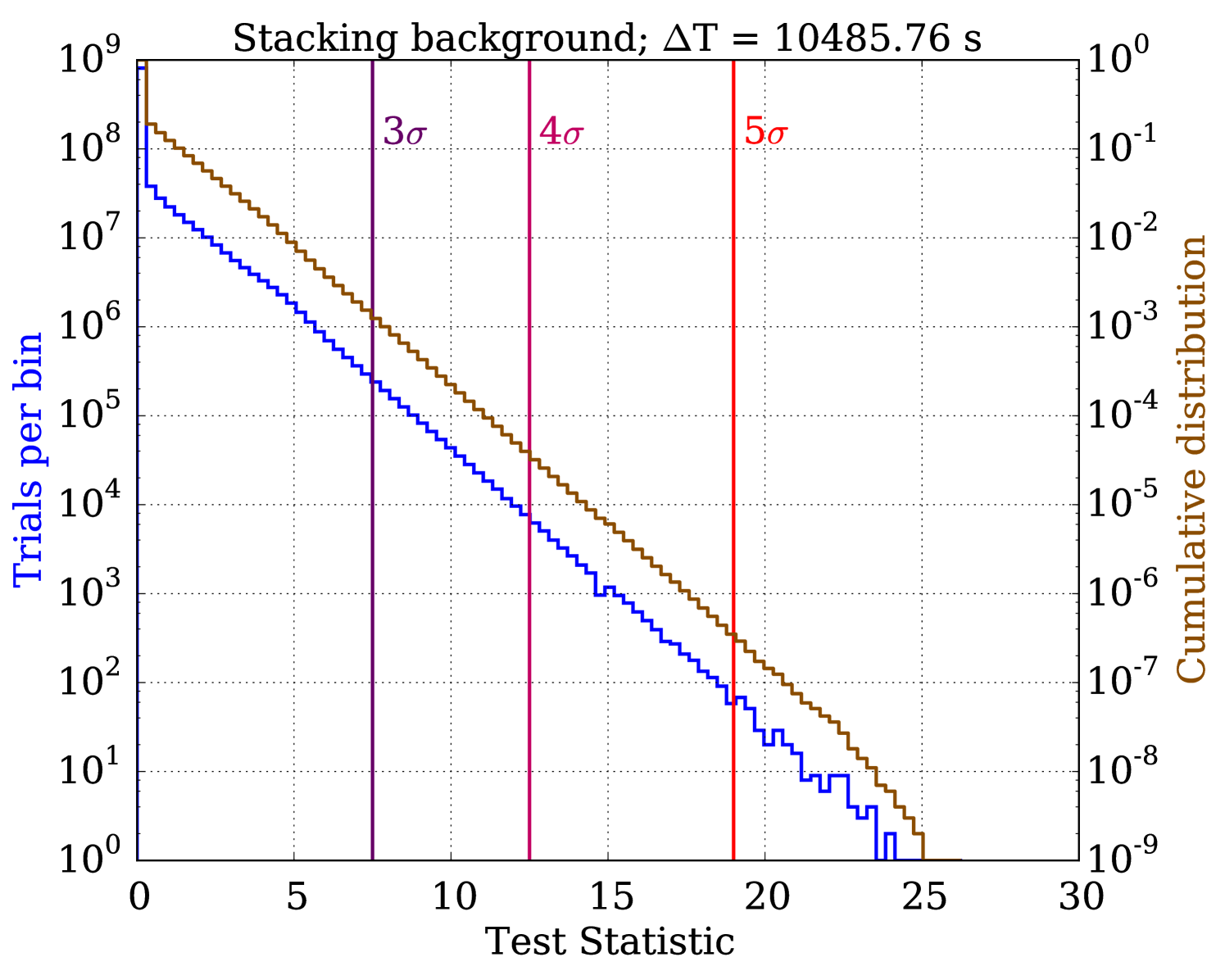
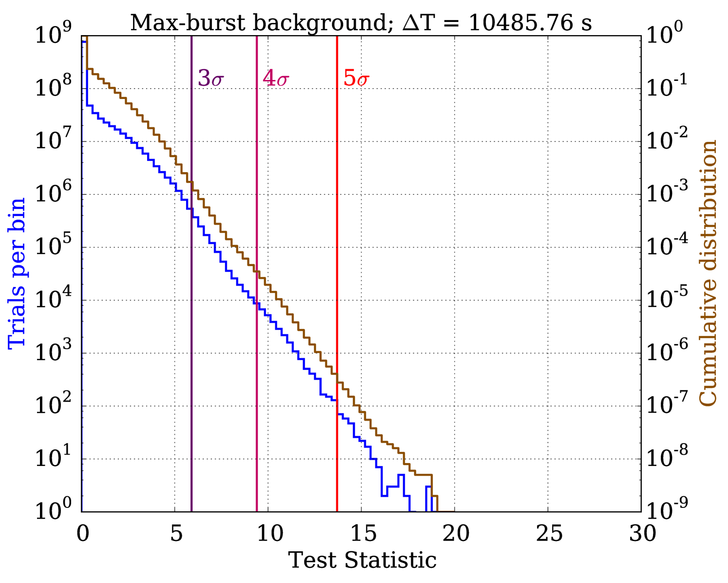
For each search method and hemisphere, we simulate $10^{9}$ background-only Monte Carlo pseudo-experiments for every $\Delta$ T. This is done by first finding the seasonal variation-adjusted background rate (from Figure 1) for each FRB in the hemisphere. The product of these rates and $\Delta$ T gives a set of mean values for the Poisson distributions from which background events will be drawn. In a single trial, the number of events in the time window of each FRB is randomly drawn, and each event is assigned spatial coordinates which are uniform in detector azimuth and have declination values drawn from the PDFs shown in Figure 2. An angular uncertainty for each event is also randomly assigned from the angular distribution of the off-time data (Maunu, 2016). The TS value for the trial is maximized with respect to $n_{s}$ and the process is repeated for $10^{9}$ trials, forming a TS distribution for the background-only hypothesis.

For example, Figure 4 shows the background-only TS distribution for the southern stacking search at $\Delta\textrm{T}=10485.76~\textrm{s}$ . Negative TS values are rounded to zero for the purposes of calculating the significance of analysis results. Building a TS distribution in this manner implicitly factors in a trials factor for the number of bursts searched, since increasing the number of sources inflates the TS values of both the analysis result and the background-only distribution. However, there is an additional trials factor when searching in overlapping time windows, so the cross-time-window trials factor must be accounted for when calculating significance values.

For each search, the analysis procedure returns the most optimal time window and the corresponding TS- $n_{s}$ pair, as determined by the p-value of the observed TS in the background-only distribution. Post-trial p-values are obtained by investigating more ensembles of background-only trials. For each trial, a set of events is injected for the largest $\Delta$ T following the background-only procedure described above. Then, for each $\Delta$ T, a TS value is calculated relative to its corresponding subset of events which are randomly selected from the total event set. The most significant of these TS values has a p-value which becomes one background-only pre-trial p-value. These trials are repeated $10^{5}$ times, forming a pre-trial p-value distribution. The position of the pre-trial p-value from the search on on-time data in this distribution determines its post-trial p-value.

4 Sensitivity

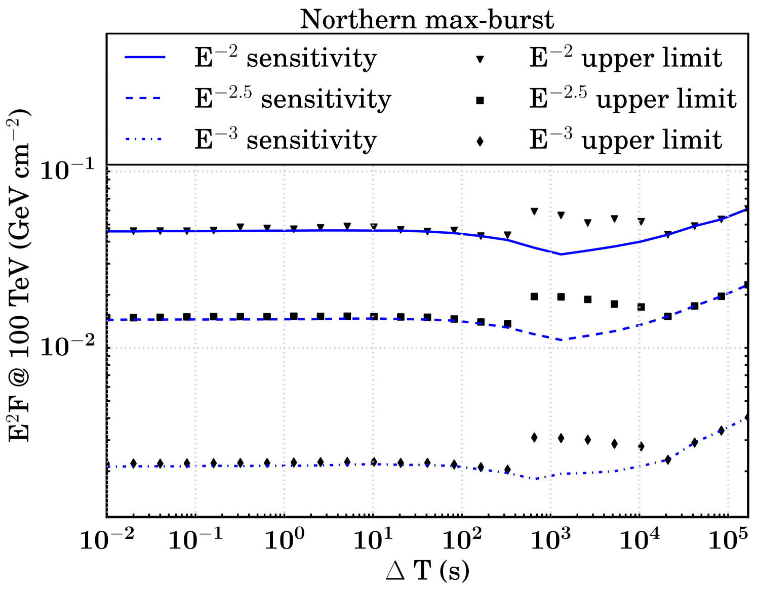
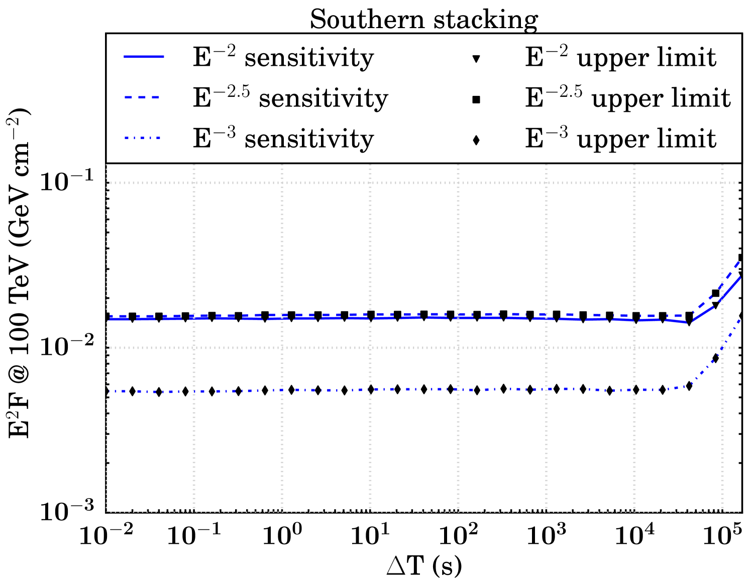
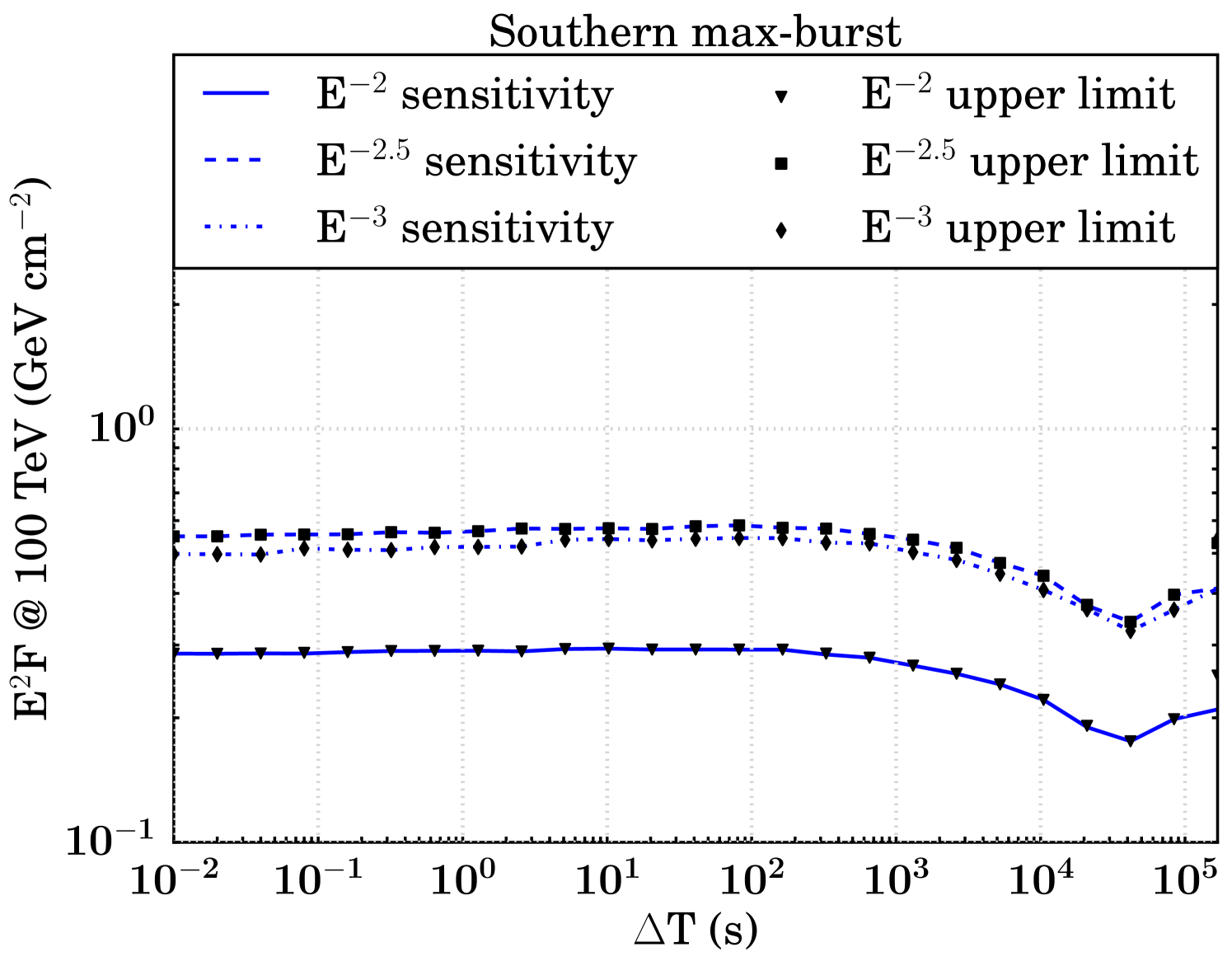
The sensitivity and discovery potential are calculated by injecting signal events following an assumed unbroken power law energy spectrum ( $E^{-2}$ , $E^{-2.5}$ , and $E^{-3}$ ) on top of injected background events. The injected signal fluence (time integrated flux, denoted as $F$ ) is found which yields a certain probability of obtaining a certain significance in the background-only TS distribution (Neyman, 1937; Aartsen et al. (2017b), IceCube Collaboration). Specifically, sensitivity and discovery potential are defined as the minimum signal fluences required to surpass, respectively, the median in 90 $\%$ of the trials and the $5\sigma$ point in 90 $\%$ of the trials. Figure 5 shows the sensitivities and $5\sigma$ discovery potentials for both hemispheres and search strategies. The searches in the northern hemisphere are roughly an order of magnitude more sensitive than those in the south, because of the differences in effective area as described in Section 2.

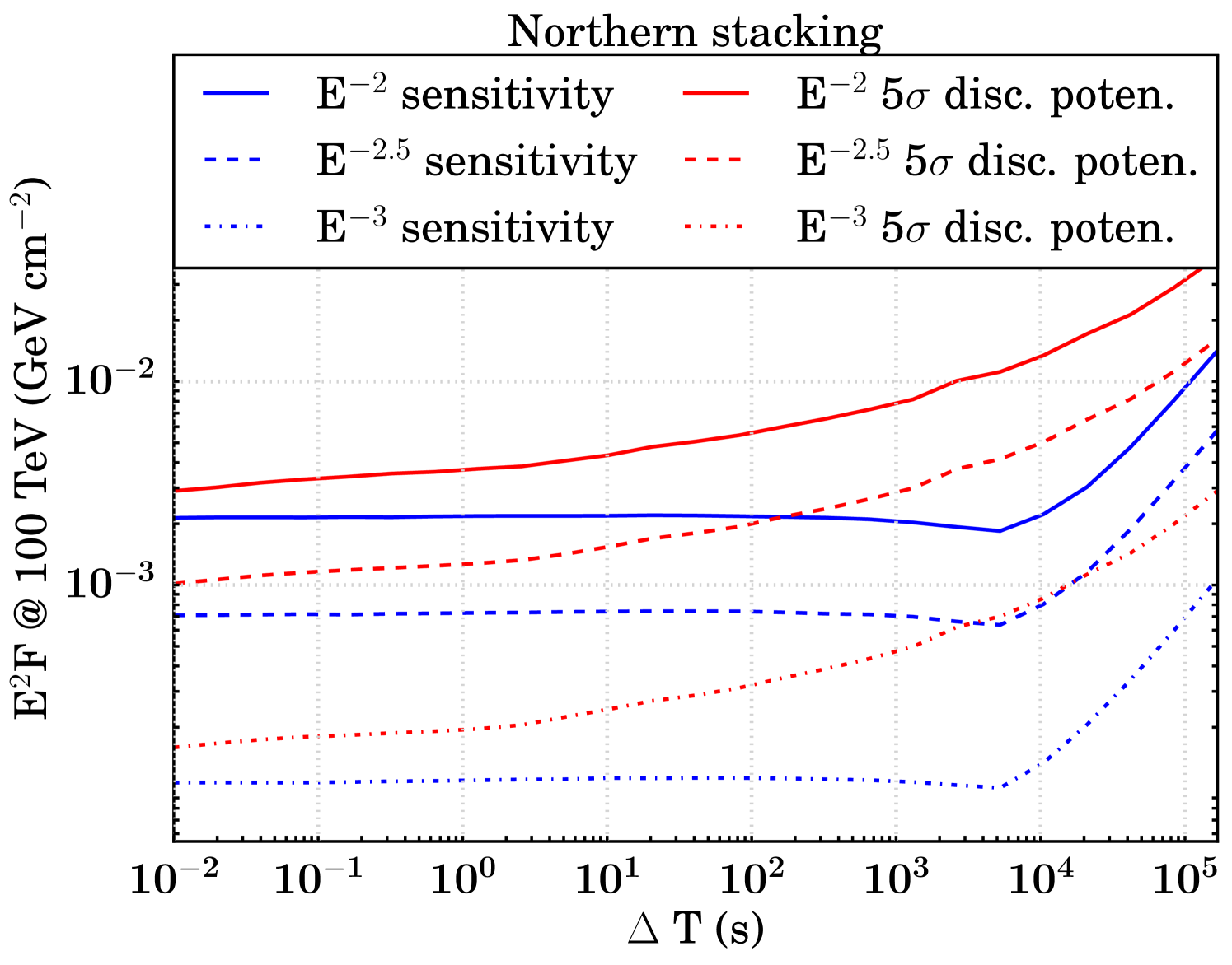
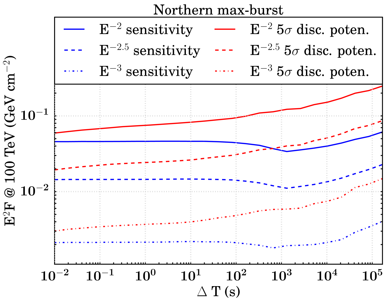
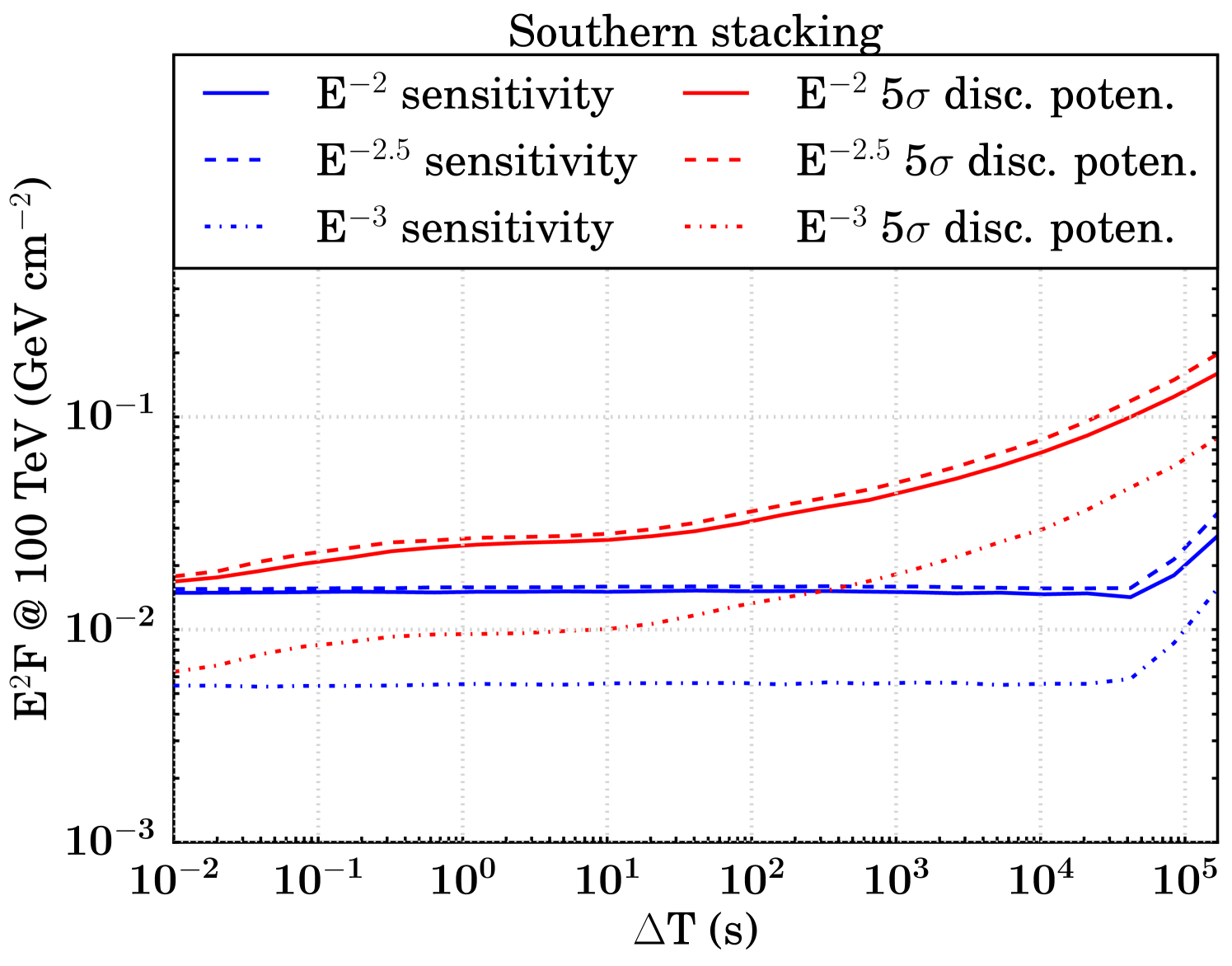
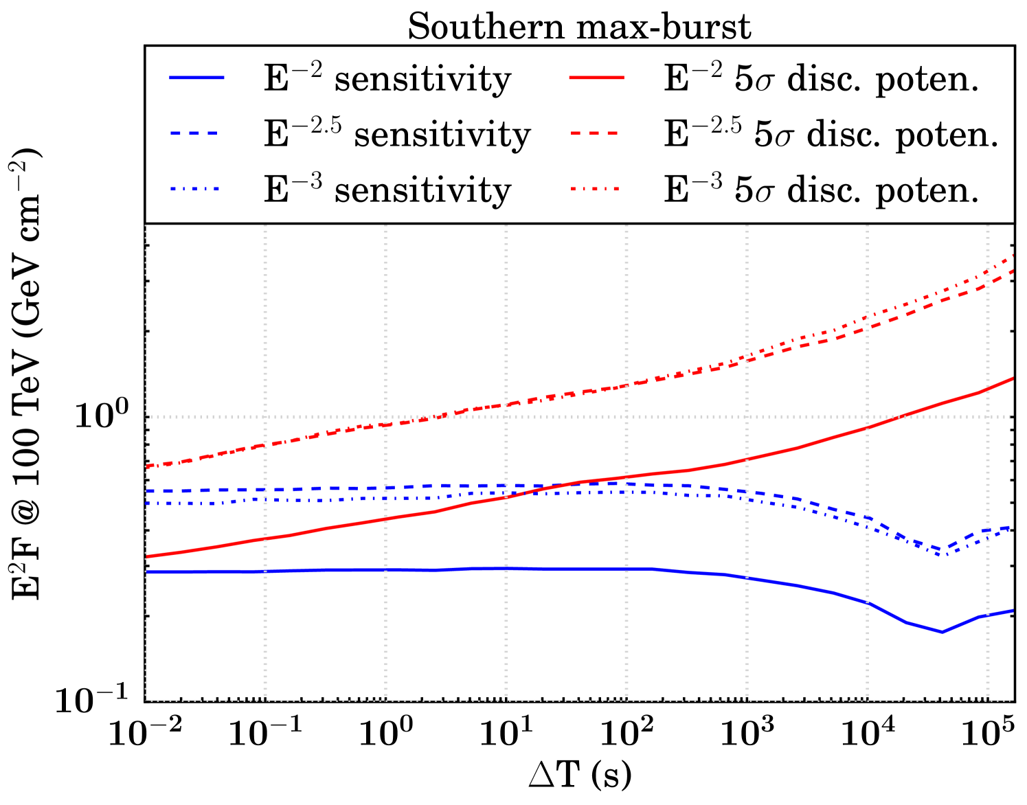
At $\Delta\textrm{T}=0.01~\textrm{s}$ , we expect fewer than 0.001 background events all-hemisphere per trial in each search. As a result, the median background-only TS value is zero for all $\Delta$ T until it becomes more probable than not that a background event is injected near an FRB location, resulting in a non-zero TS value. In general, the sensitivity remains constant in a $\Delta$ T range that is relatively background-free and transitions to a monotonically increasing function in background-dominated $\Delta$ T. We still search all of these low-background $\Delta$ T because the discovery potential increases even in the small background regime (Figure 5).

As a result of our methodology, there is a point in the background transition region where the sensitivity fluence appears to improve. Where the median of the background TS distribution is zero, the 90% sensitivity threshold for signal injection remains constant. But when $\Delta$ T is growing, there are more background events in each trial which can give rise to non-zero TS values, so the injected fluence necessary to meet the criteria for sensitivity is less. Once the median background TS value becomes non-zero, the sensitivity increases as expected.

5 Results

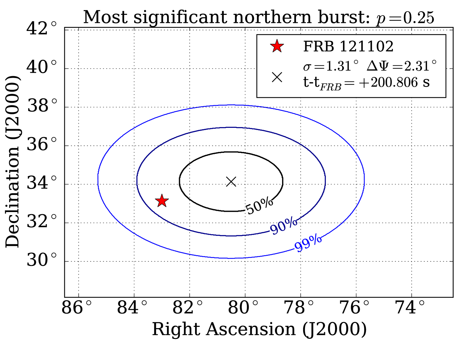
After correcting for trials factors induced by 25 overlapping time windows searched, no significant correlation between neutrino events and FRBs is found (nor with the LOFAR burst). The most significant pre-trial p-value ( $p=0.034$ ) is found in the northern max-burst search at ${\Delta\textrm{T}=655.36~\textrm{s}}$ , with best-fit TS and $n_{s}$ of 3.90 and 0.99 respectively. The post-trial p-value for this search is $p=0.25$ . In the same $\Delta$ T, the northern stacking search returned a best-fit TS and $n_{s}$ of 1.41 and 1.01 respectively, corresponding to a pre-trial p-value $p=0.074$ and post-trial p-value $p=0.375$ . The most signal-like event for both searches occurred 200.806 s after FRB 121102 b3, with an angular separation of 2.31^∘ and estimated angular uncertainty of 1.31^∘.

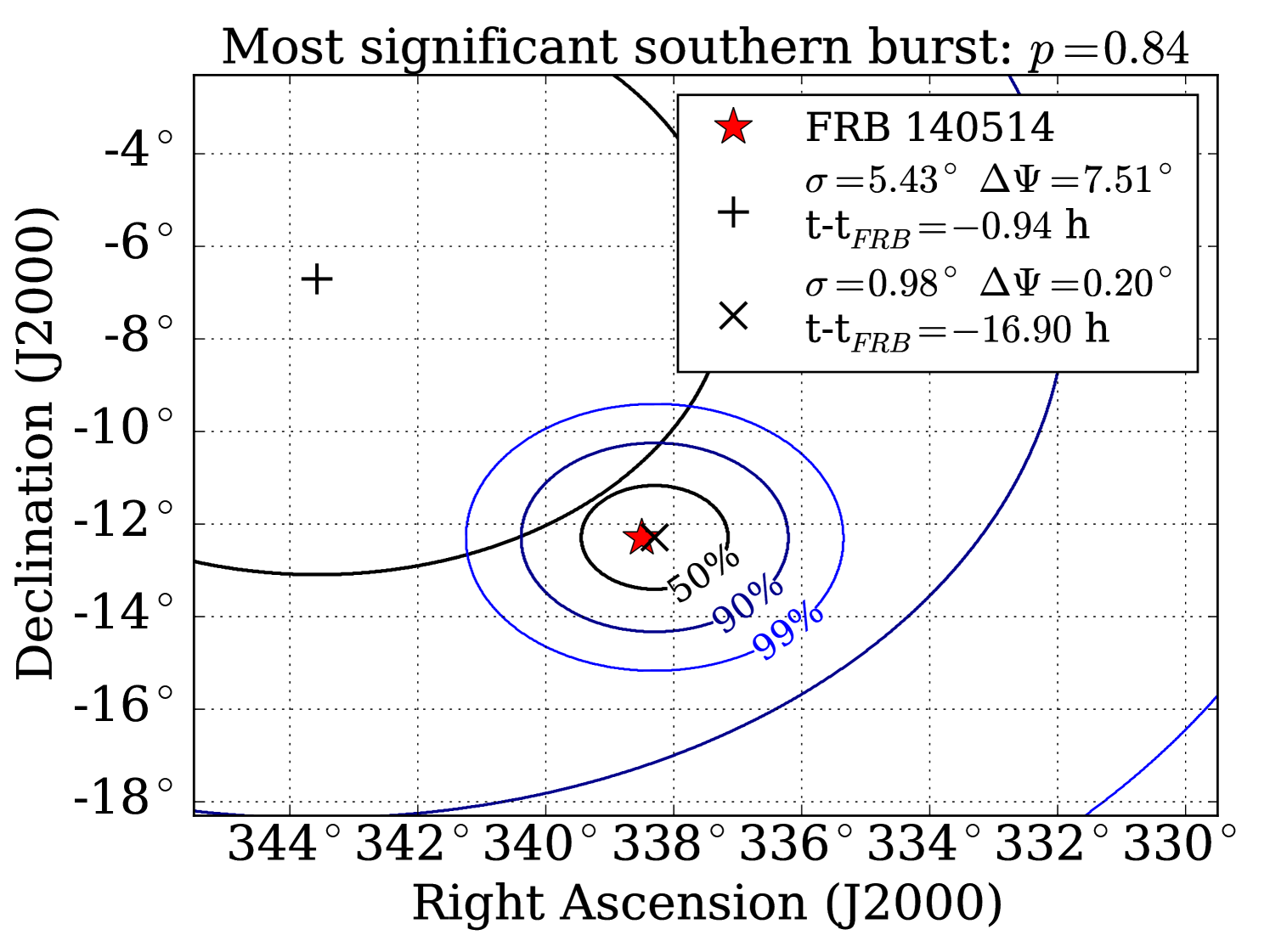
In the southern hemisphere, the max-burst search returns the most significant pre-trial p-value ( $p=0.412$ ) at ${\Delta\textrm{T}=167772.16~\textrm{s}}$ with TS and $n_{s}$ of 0.64 and 0.78, for a post-trial p-value of $p=0.84$ . In the southern stacking search, no TS value greater than zero was ever obtained for all $\Delta$ T. Even for the largest $\Delta$ T, where the southern max-burst search returned a positive TS value at one FRB, the order-of-magnitude increase in background for 9 FRBs stacked sufficiently diminished the significance of the events. Analysis results are summarized in Table 3, and sky maps of the events which most contributed to the results of each hemisphere are shown in Figure 6.

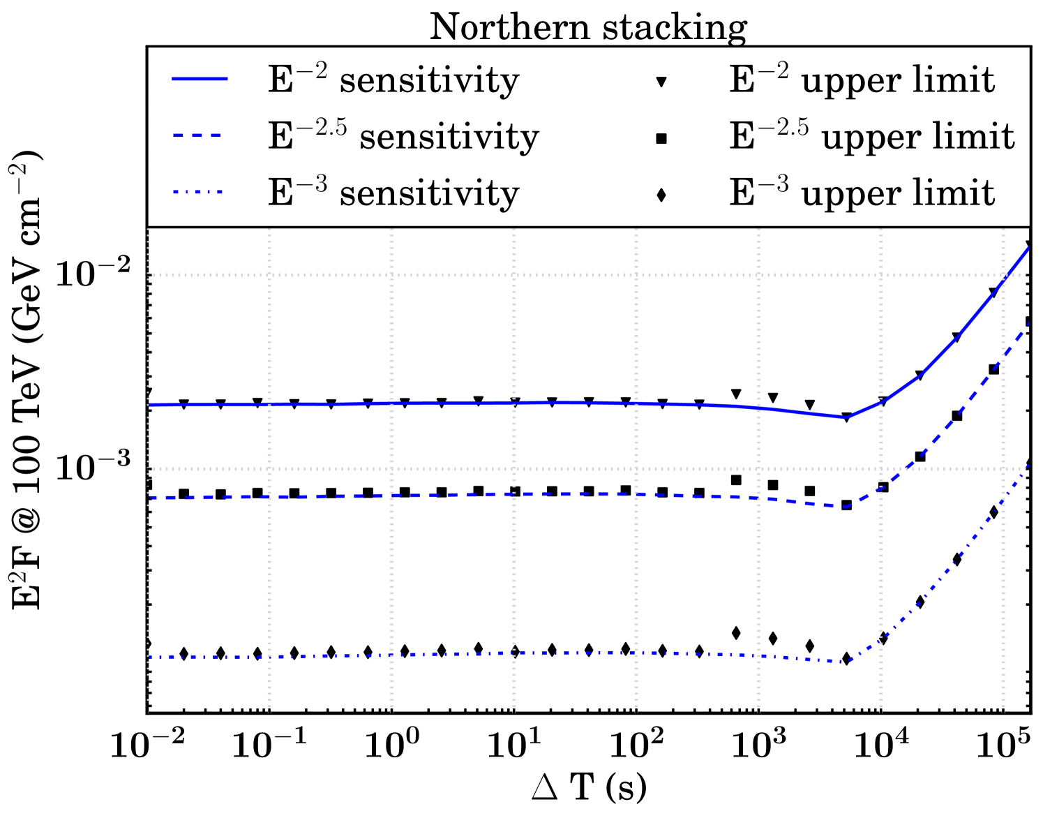
To set upper limits on the neutrino emission from FRBs, we use the same method which determines sensitivity, using the observed TS rather than the background-only median as a significance threshold. For most $\Delta$ T, both the background median and analysis result TS values are zero, resulting in an upper limit equal to the sensitivity (Figure 7). The northern stacking search returned the most constraining 90% confidence level upper limit for $E^{-2}$ neutrino emission from FRBs among all four searches in this analysis, ${E^{2}F=0.0021~\textrm{GeV}~\textrm{cm}^{-2}}$ per burst.

This process has been repeated for each source separately to calculate per-burst upper limits (see Table 4). $E^{-2}$ fluence upper limits were determined by running background and signal-injection trials for a source list containing only one FRB, repeated for each unique source and for each year in which FRB 121102 was detected.

Table 3: Analysis results are summarized for searches in both the northern and southern hemispheres. Where a most significant TS is found, the timing and directional separation of the event which most contributed to that TS value are provided. In the southern stacking test, the TS values for all time windows are zero; there is no

\Delta

T searched which is more signal-like than background-like.

Northern ( $\delta>-5^{\circ}$ )	best fit TS	best fit $n_{s}$	most significant event ( $t-t_{\mathrm{FRB}}$ , $\Delta\Psi$ )	pre-trial $p$ (post-trial $p$ )	optimal $\Delta$ T	coincident FRB
max-burst test	3.90	0.99	(+200.806 s, 2.31^∘)	0.034 (0.25)	655.36 s	FRB121102 repeater 2015/06/02 16:38:07.575 UTC
stacking test	1.41	1.01	(+200.806 s, 2.31^∘)	0.074 (0.375)	655.36 s	FRB121102 repeater 2015/06/02 16:38:07.575 UTC
Southern ( $\delta<-5^{\circ}$ )	best fit TS	best fit $n_{s}$	most significant event ( $t-t_{\mathrm{FRB}}$ , $\Delta\Psi$ )	pre-trial $p$ (post-trial $p$ )	optimal $\Delta$ T	coincident FRB
max-burst test	0.64	0.78	(-16.9 hrs, 0.20^∘)	0.412 (0.84)	167772.16 s	FRB 140514 2014/05/14 17:14:11.06 UTC
stacking test	0	0	–	1.0 (1.0)	–	–

Table 4: Neutrino fluence upper limits (90% confidence) are constructed assuming an

E^{-2}

spectrum. The limits have been calculated for each burst individually for the

\Delta

~=~0.01

s time window and are shown here as

E^{2}F

. Each burst from FRB 121102 has a limit corresponding to the year of data during which it was detected.

FRB	Dec	E^-2 fluence upper limit (GeV cm^-2)
FRB 121002	-85^∘ 11^′	1.16
FRB 131104	-51^∘ 17^′	1.03
FRB 110627	-44^∘ 44^′	0.963
FRB 150418	-19^∘ 00^′	0.331
FRB 120127	-18^∘ 25^′	0.318
FRB 110220	-12^∘ 24^′	0.184
FRB 140514	-12^∘ 18^′	0.192
FRB 130626	-07^∘ 27^′	0.153
FRB 130729	-05^∘ 59^′	0.136
FRB 110703	-02^∘ 52^′	0.0575
FRB 110523	-00^∘ 12^′	0.0578
FRB 130628	03^∘ 26^′	0.0643
FRB 121102 b0	33^∘ 05^′	0.0932
FRB 121102 b1-b2	33^∘ 05^′	0.0925
FRB 121102 b3-b16	33^∘ 05^′	0.0919
LOFAR transient	86^∘ 22^′	0.164

6 Conclusion and Outlook

In a search for muon neutrinos from 29 FRBs detected from 2010 May 31 to 2016 May 12, no significant correlation has been found. In both hemispheres, several events were found to be spatially coincident with some FRBs but also consistent with background.

Therefore, we set upper limits on neutrino emission from FRBs as a function of time window searched. For a $E^{-2}$ energy spectrum, the most stringent limit on neutrino fluence per burst is ${E^{2}F=0.0021~\textrm{GeV}~\textrm{cm}^{-2}}$ , obtained from the shortest time window (10 ms) in the northern stacking search. This limit is much improved in comparison to a previous search with only one year of IceCube data and using a binned likelihood method (Fahey et al., 2017). The limits set in this paper are also the most constraining ones on neutrinos from FRBs for neutrino energies above 1 TeV.

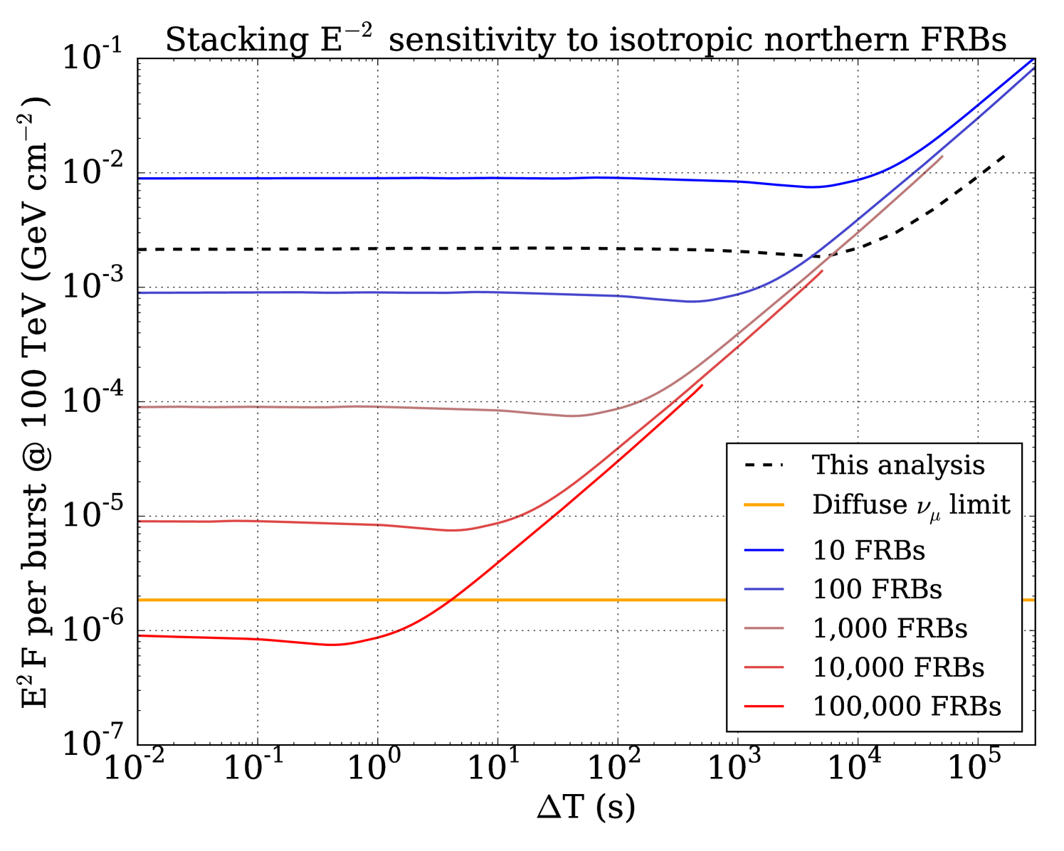
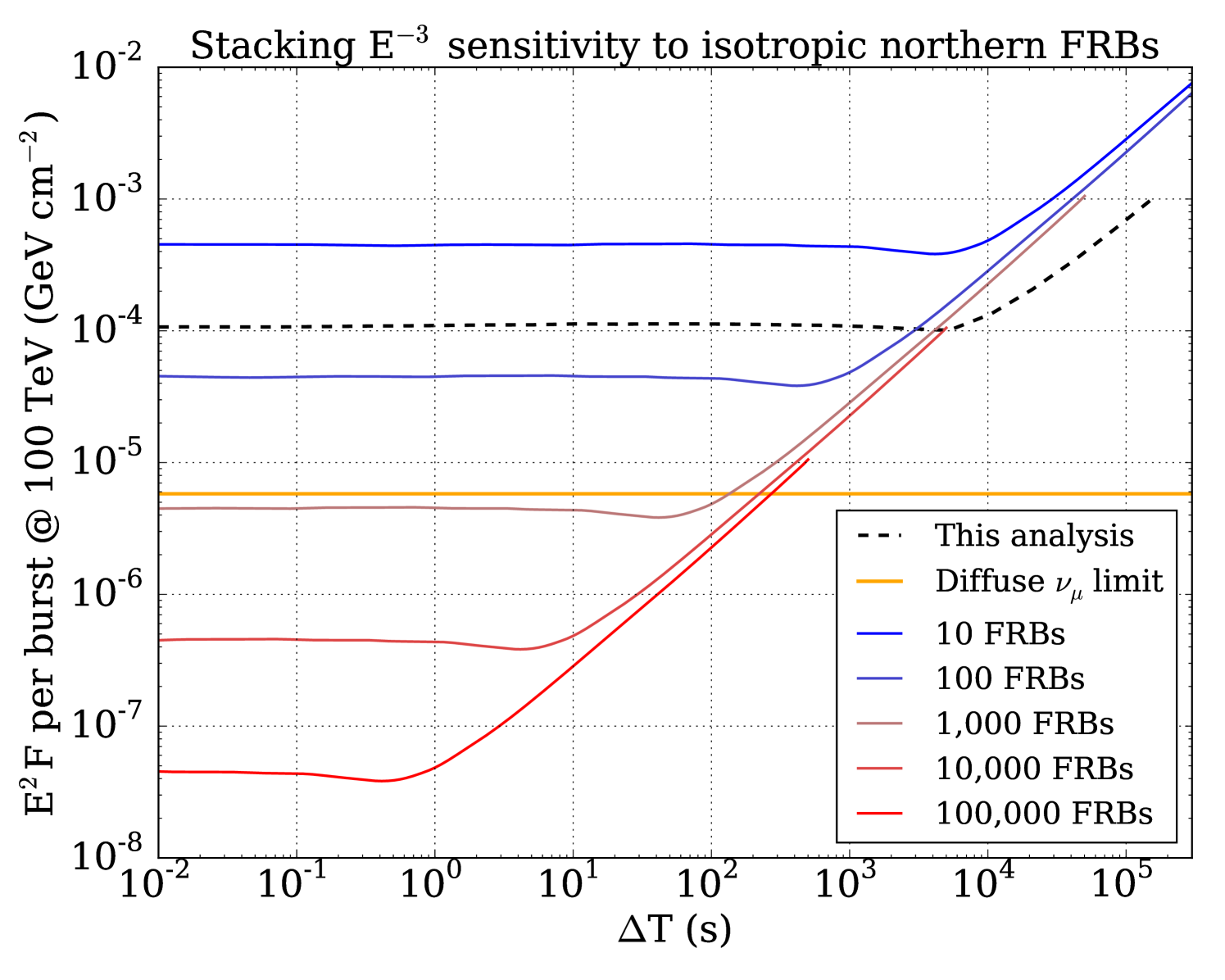
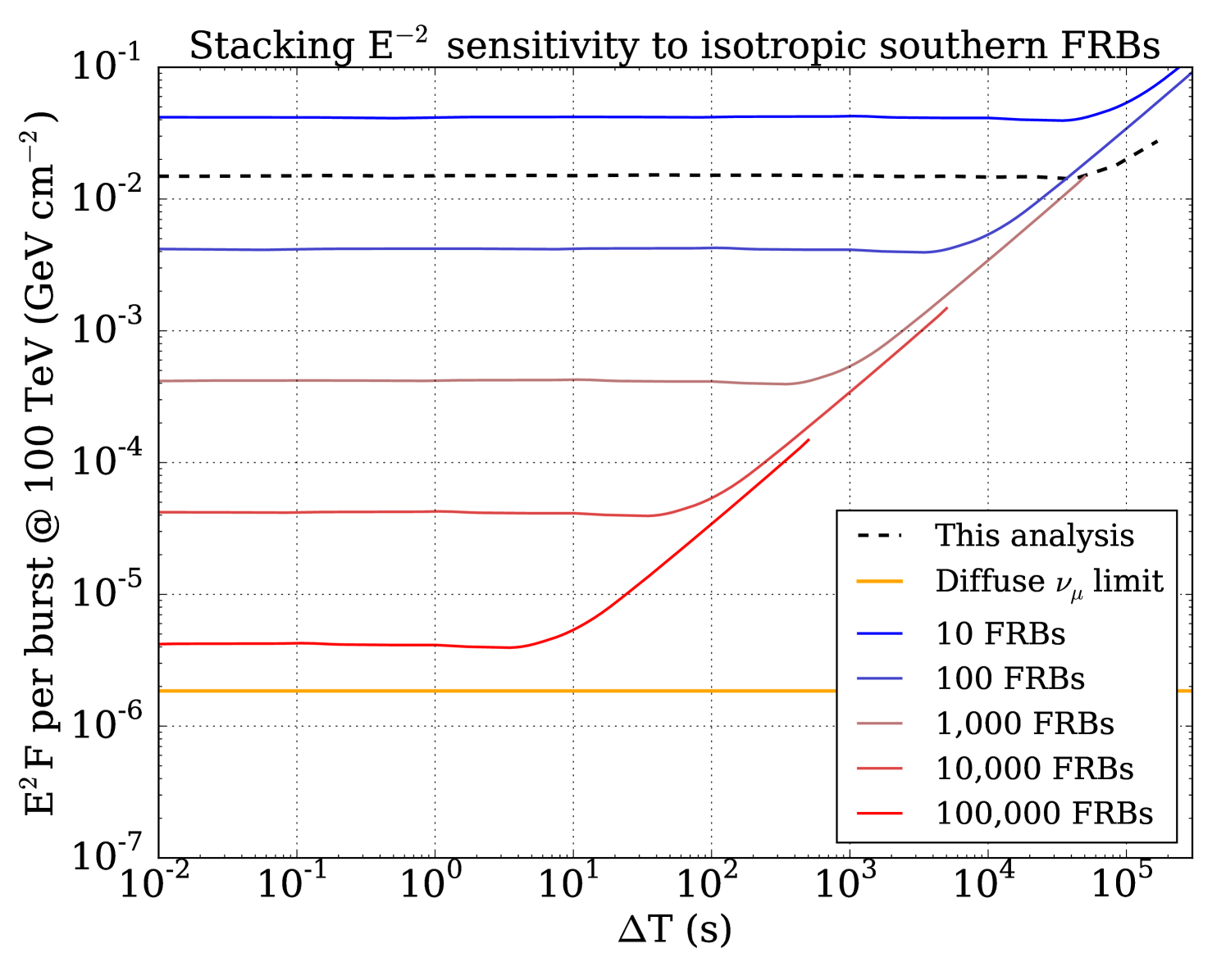
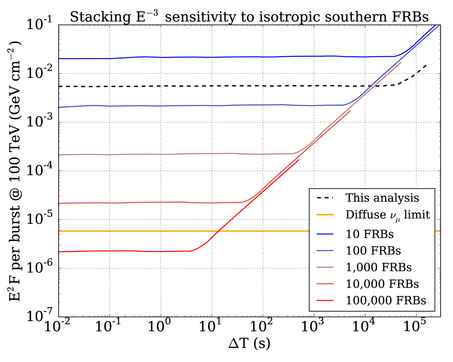
At the moment, we can set even more constraining limits on high-energy neutrino emission from FRBs using IceCube’s astrophysical $\nu_{\mu}$ flux measurement (Aartsen et al. (2016a), IceCube Collaboration), assuming the current catalog of detected FRBs is representative of a homogeneous source class. Using an estimated all-sky FRB occurrence rate of 3,000 sky^-1 day^-1 (Macquart & Ekers, 2017), the $\nu_{\mu}$ fluence per FRB at 100 TeV cannot exceed $E^{2}F=1.9\cdot 10^{-6}$ GeV cm^-2 for an emission spectrum of $E^{-2}$ ; otherwise, FRBs would contribute more than the entire measured astrophysical $\nu_{\mu}$ flux. The astrophysical flux used here is extrapolated from a fit at energies of 194 TeV – 7.8 PeV, so it is only a rough estimate of the maximum neutrino emission from FRBs in the energy range this analysis concerns.

With newly operating radio observatories like CHIME (CHIME Scientific Collaboration, 2017), we expect on the order of 1,000 FRBs to be discovered quasi-isotropically each year, which will improve the sensitivity of IceCube to a follow-up stacking search by orders of magnitude (Figure 8). Future analyses using IceCube data may also benefit from a more inclusive dataset, allowing a higher overall rate of muon-like and cascade-like events in exchange for increased sensitivity at $\Delta$ T $~<~1,000$ s. Cascade-like events do not contain muons, and as a result provide an angular resolution on the order of $10^{\circ}$ . However, a coincident event may still provide potential for high significance in very short time windows, where background is low. Furthermore, if some sub-class of FRBs is associated with nearby supernovae, MeV-scale neutrinos can be searched in the IceCube supernova stream which looks for a sudden increase in the overall noise rate of the detector modules (Abbasi et al. (2011), IceCube Collaboration).

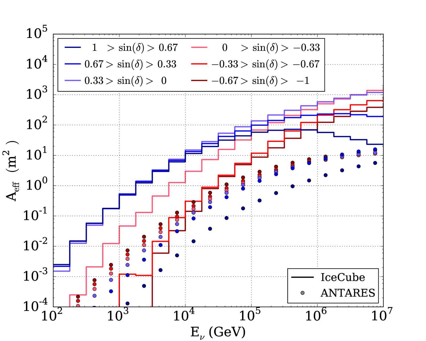
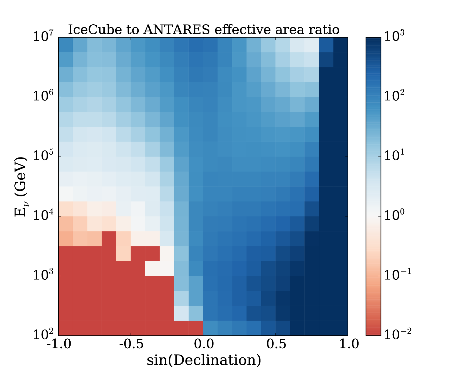
The ANTARES neutrino observatory is most sensitive in the southern hemisphere, where the majority of FRB sources have been detected to date. Higher FRB detection rate (due to more observation time) from the southern hemisphere also provides ANTARES the opportunities for rapid follow-up observations when FRBs are caught in real time (Petroff et al., 2017). However, we emphasize that IceCube also has excellent sensitivity in much of the southern hemisphere. In Figure 9, we provide a quantitative comparison of the effective areas of the two observatories, which can serve as a useful reference when future FRBs are detected at arbitrary declinations. At energies above 50 TeV, the effective area of IceCube to neutrinos is the highest of any neutrino observatory across the entire ( $4\pi$ ) sky (Figure 9). For ${E_{\nu}<50}$ TeV, particularly where ${\sin(\delta)<-0.33}$ , ANTARES complements IceCube in searches for isotropic transient sources, achieving greater effective area in $1/3$ of the sky. Since ANTARES is not located at a pole, the zenith angle of any astrophysical source changes throughout the day, thus detector overburden and sensitivity are time-dependent. Therefore, the effective areas provided by ANTARES for a given declination band are the day-averaged values (Adrian-Martinez et al., 2014). A joint stacking analysis between IceCube and ANTARES (Adrian-Martinez et al., 2016a, b) could maximize the sensitivity of neutrino searches from FRBs across the full sky. Furthermore, with the implementation of the expanding time window techniques, IceCube can now follow up on generic fast transients rapidly, enabling monitoring of the transient sky in the neutrino sector (Aartsen et al. (2017f), IceCube Collaboration).

The authors gratefully acknowledge the support from the following agencies and institutions: USA – U.S. National Science Foundation-Office of Polar Programs, U.S. National Science Foundation-Physics Division, Wisconsin Alumni Research Foundation, Center for High Throughput Computing (CHTC) at the University of Wisconsin–Madison, Open Science Grid (OSG), Extreme Science and Engineering Discovery Environment (XSEDE), U.S. Department of Energy–National Energy Research Scientific Computing Center, Particle astrophysics research computing center at the University of Maryland, Institute for Cyber-Enabled Research at Michigan State University, and Astroparticle physics computational facility at Marquette University; Belgium – Funds for Scientific Research (FRS-FNRS and FWO), FWO Odysseus and Big Science programmes, and Belgian Federal Science Policy Office (Belspo); Germany – Bundesministerium für Bildung und Forschung (BMBF), Deutsche Forschungsgemeinschaft (DFG) and the German Excellence Initiative, Helmholtz Alliance for Astroparticle Physics (HAP), Initiative and Networking Fund of the Helmholtz Association, Deutsches Elektronen Synchrotron (DESY), and High Performance Computing cluster of the RWTH Aachen; Sweden – Swedish Research Council, Swedish Polar Research Secretariat, Swedish National Infrastructure for Computing (SNIC), and Knut and Alice Wallenberg Foundation; Australia – Australian Research Council; Canada – Natural Sciences and Engineering Research Council of Canada, Calcul Québec, Compute Ontario, Canada Foundation for Innovation, WestGrid, and Compute Canada; Denmark – Villum Fonden, Danish National Research Foundation (DNRF); New Zealand – Marsden Fund; Japan - Japan Society for Promotion of Science (JSPS) and Institute for Global Prominent Research (IGPR) of Chiba University; Korea – National Research Foundation of Korea (NRF); Switzerland – Swiss National Science Foundation (SNSF).

References

Aartsen et al. (2013a) (IceCube Collaboration) Aartsen et al. (IceCube Collaboration). 2013a, Science, 342
Aartsen et al. (2013b) (IceCube Collaboration) —. 2013b, Phys. Rev. Lett., 111, 021103
Aartsen et al. (2013c) (IceCube Collaboration) —. 2013c, proc. 33rd ICRC, 0492
Aartsen et al. (2014) (IceCube Collaboration) —. 2014, Phys. Rev. Lett., 113, 101101
Aartsen et al. (2015a) (IceCube Collaboration) —. 2015a, Phys. Rev. D, 91, 022001
Aartsen et al. (2015b) (IceCube Collaboration) —. 2015b, Astrophys. J., 809, 98
Aartsen et al. (2015c) (IceCube Collaboration) —. 2015c, Phys. Rev. Lett., 115, 081102
Aartsen et al. (2015d) (IceCube Collaboration) —. 2015d, Phys. Rev. Lett., 114, 171102
Aartsen et al. (2015e) (IceCube Collaboration) —. 2015e, Astrophys. J. Lett., 805, L5
Aartsen et al. (2015f) (IceCube Collaboration) —. 2015f, Astrophys. J., 805, L5
Aartsen et al. (2016a) (IceCube Collaboration) —. 2016a, Astrophys. J., 833, 3
Aartsen et al. (2016b) (IceCube Collaboration) —. 2016b, Phys. Rev., D93, 022001
Aartsen et al. (2017a) (IceCube Collaboration) —. 2017a, Astrophys. J., 835, 151
Aartsen et al. (2017b) (IceCube Collaboration) —. 2017b, Astrophys. J., 843, 112
Aartsen et al. (2017c) (IceCube Collaboration) —. 2017c, Astrophys. J., 835, 45
Aartsen et al. (2017d) (IceCube Collaboration) —. 2017d, arXiv:1710.01191 [astro-ph.HE]
Aartsen et al. (2017e) (IceCube Collaboration) —. 2017e, JINST, 12, P03012
Aartsen et al. (2017f) (IceCube Collaboration) —. 2017f, Astropart. Phys., 92, 30
Abbasi et al. (2011) (IceCube Collaboration) Abbasi et al. (IceCube Collaboration). 2011, Astron. Astrophys., 535, A109, [Erratum: Astron. Astrophys.563,C1(2014)]
Abbasi et al. (2012) (IceCube Collaboration) —. 2012, Nature, 484, 351
Adrian-Martinez et al. (2014) Adrian-Martinez, S., et al. 2014, Astrophys. J., 786, L5
Adrian-Martinez et al. (2016a) —. 2016a, Phys. Rev., D93, 122010
Adrian-Martinez et al. (2016b) —. 2016b, Astrophys. J., 823, 65
Argüelles et al. (2015) Argüelles, C. A., Katori, T., & Salvado, J. 2015, Phys. Rev. Lett., 115, 161303
Bannister et al. (2017) Bannister, K., Shannon, R., Macquart, J., et al. 2017, Astrophys. J., 841, L12
Berezinsky et al. (2009) Berezinsky, V., Olum, K. D., Sabancilar, E., & Vilenkin, A. 2009, Phys. Rev., D80, 023014
Bustamante et al. (2015) Bustamante, M., Beacom, J. F., & Winter, W. 2015, Phys. Rev. Lett., 115, 161302
Caleb et al. (2017) Caleb, M., Flynn, C., Bailes, M., et al. 2017, Mon. Not. Roy. Astron. Soc., 468, 3746
Chatterjee et al. (2017) Chatterjee, S., Law, C. J., Wharton, R. S., et al. 2017, Nature, 541, 58
CHIME Scientific Collaboration (2017) CHIME Scientific Collaboration. 2017, Astrophys. J., 844, 161
Cordes et al. (2016) Cordes, J. M., Wharton, R. S., Spitler, L. G., Chatterjee, S., & Wasserman, I. 2016, arXiv:1605.05890 [astro-ph.HE]
Fahey et al. (2017) Fahey, S., Kheirandish, A., Vandenbroucke, J., & Xu, D. 2017, Astrophys. J., 845, 14
Falcke & Rezzolla (2014) Falcke, H., & Rezzolla, L. 2014, Astron. Astrophys., 562, A137
Li et al. (2014) Li, X., Zhou, B., He, H.-N., Fan, Y.-Z., & Wei, D.-M. 2014, Astrophys. J., 797, 33
Lorimer et al. (2007) Lorimer, D. R., Bailes, M., McLaughlin, M. A., Narkevic, D. J., & Crawford, F. 2007, Science, 318, 777
Lunardini & Sabancilar (2012) Lunardini, C., & Sabancilar, E. 2012, Phys. Rev., D86, 085008
Macquart & Ekers (2017) Macquart, J.-P., & Ekers, R. 2017, arXiv:1710.11493 [astro-ph.HE]
Masui et al. (2015) Masui, K., Lin, H.-H., Sievers, J., et al. 2015, Nature, 528, 523
Maunu (2016) Maunu, R. 2016, PhD thesis, University of Maryland (College Park, Md.)
Murase et al. (2016) Murase, K., Kashiyama, K., & Mészáros, P. 2016, Mon. Not. Roy. Astron. Soc., 461, 1498
Neyman (1937) Neyman, J. 1937, Phil. Trans. Roy. Soc. Lond., A236, 333
Petroff et al. (2017) Petroff, E., et al. 2017, Mon. Not. Roy. Astron. Soc., 469, 4465
Rees (1977) Rees, M. J. 1977, Nature, 266, 333
Scholz et al. (2016) Scholz, P., Spitler, L. G., Hessels, J. W. T., et al. 2016, Astrophys. J., 833, 177
Spitler et al. (2014) Spitler, L. G., Cordes, J. M., Hessels, J. W. T., et al. 2014, Astrophys. J., 790, 101
Stewart et al. (2016) Stewart, A. J., Fender, R. P., Broderick, J. W., et al. 2016, Mon. Not. Roy. Astron. Soc., 456, 2321
Thornton et al. (2013) Thornton, D., Stappers, B., Bailes, M., et al. 2013, Science, 341, 53
Totani (2013) Totani, T. 2013, Pub. Astron. Soc. Jpn., 65, L12
Ye et al. (2017) Ye, J., Wang, K., & Cai, Y.-F. 2017, Eur. Phys. J., C77, 720