A Sequential Subspace Method for Millimeter Wave MIMO Channel Estimation
Abstract
Data transmission over the millimeter wave (mmWave) in fifth-generation wireless networks aims to support very high speed wireless communications. A substantial increase in spectrum efficiency for mmWave transmission can be achieved by using advanced hybrid analog-digital precoding, for which accurate channel state information (CSI) is the key. Rather than estimating the entire channel matrix, it is now well-understood that directly estimating subspace information, which contains fewer parameters, does have enough information to design transceivers. However, the large channel use overhead and associated computational complexity in the existing channel subspace estimation techniques are major obstacles to deploy the subspace approach for channel estimation. In this paper, we propose a sequential two-stage subspace estimation method that can resolve the overhead issues and provide accurate subspace information. Utilizing a sequential method enables us to avoid manipulating the entire high-dimensional training signal, which greatly reduces the computational complexity. Specifically, in the first stage, the proposed method samples the columns of channel matrix to estimate its column subspace. Then, based on the obtained column subspace, it optimizes the training signals to estimate the row subspace. For a channel with receive antennas and transmit antennas, our analysis shows that the proposed technique only requires channel uses, while providing a guarantee of subspace estimation accuracy. By theoretical analysis, it is shown that the similarity between the estimated subspace and the true subspace is linearly related to the signal-to-noise ratio (SNR), i.e., , at high SNR, while quadratically related to the SNR, i.e., , at low SNR. Simulation results show that the proposed sequential subspace method can provide improved subspace accuracy, normalized mean squared error, and spectrum efficiency over existing methods.
Index Terms:
Channel estimation, compressed sensing, millimeter wave communication, multi-input multi-output, subspace estimation.I Introduction
Wireless communications using the millimeter wave (mmWave), which occupies the frequency band (30–300 GHz), address the current scarcity of wireless broadband spectrum and enable high speed transmission in fifth-generation (5G) wireless networks [1]. Due to the short wavelength, it is possible to employ large-scale antenna arrays with small-form-factor [2, 3, 4]. To reduce power consumption and hardware complexity, the mmWave systems exploit hybrid analog-digital multiple-input multiple-output (MIMO) architecture operating with a limited number of radio frequency (RF) chains [2]. Under the perfect channel state information (CSI), it has been shown that hybrid precoding can achieve nearly optimal performance as fully-digital precoding [2, 3, 5]. In practice, accurate CSI must be estimated via channel training in order to have effective precoding for robust mmWave MIMO transmission. However, extracting accurate CSI in the mmWave MIMO poses new challenges due to the limited number of RF chains that limits the observability of the channel and greatly increases the channel use overhead.
To reduce the channel use overhead, initial works focused on the beam alignment techniques [6, 7] utilizing beam search codebooks. By exploiting the fact that mmWave propagation exhibits low-rank characteristic, recent researches formulated the channel estimation task as a sparse signal reconstruction problem [8, 9] and low-rank matrix reconstruction problem [10, 11, 12, 13, 14, 15]. By using the knowledge of sparse signal reconstruction, orthogonal matching pursuit (OMP) [8] and sparse Bayesian learning (SBL) [9] were motivated to estimate the sparse mmWave channel in angular domain. Alternatively, if the channel is rank-sparse, it is possible to directly extract sufficient channel subspace information for the precoder design [16, 10, 11]. These subspace-based methods employ the Arnoldi iteration [16] to estimate the channel subspaces and knowledge of matrix completion [10, 11] to estimate the low-rank mmWave channel information.
Though the sparse signal reconstruction [8, 9] and matrix completion [10, 11] techniques can reduce the channel use overhead compared to traditional beam alignment techniques, the training sounders of these techniques [8, 9, 10, 11] are pre-designed and high-dimensional, which leads to the fact that these works suffer from explosive computational complexity as the size of arrays grows. To reduce the computational complexity, the adaptive training techniques have been investigated in [4, 16, 17], where the training sounders can be adaptively designed based on the feedback or two-way training. But these adaptive training techniques could not guarantee the performance on mean squared error (MSE) and/or subspace estimation accuracy. Moreover, the techniques provided in [4, 16, 17] will introduce additional channel use overhead due to the required feedback and two-way training.
To resolve the feedback overhead and maintain the benefit of adaptive training, in this paper, we present a two-stage subspace estimation approach, which sequentially estimates the column and row subspaces of the mmWave MIMO channel. Compared to the existing channel estimation techniques in [8, 9, 10, 11], the training sounders of the proposed approach are adaptively designed to reduce the channel use overhead and computational complexity. Moreover, the proposed approach is open-loop, thus it has no requirements of feedback and two-way channel sounding compared to priori adaptive training techniques [4, 16, 17]. The main contributions of this paper are described as follows:
-
•
We propose a two-stage subspace estimation technique called a sequential and adaptive subspace estimation (SASE) method. In the channel estimation of the proposed SASE, the column and row subspaces are estimated sequentially. Specifically, in the first stage, we sample a small fraction of columns of the channel matrix to obtain an estimate of the column subspace of the channel. In the second stage, the row subspace of the channel is estimated based on the obtained column subspace. In particular, by using the estimated column subspace obtained in the first stage, the receive training sounders of the second stage are optimized to reduce the number of channel uses. Compared to the existing works with fixed training sounders, where the entire high-dimensional training signals are utilized to obtain the CSI, the proposed adaptation has the advantage that the dimension of signals being processed in each stage is much less than that of the entire training signal, greatly reducing the computational complexity. Thus, the proposed SASE has much less computational complexity than those of the existing methods.
-
•
We analyze the subspace estimation accuracy, which guarantees the performance of the proposed SASE technique. Through extensive analysis, it is shown that the subspace estimation accuracy of the SASE is linearly related to the signal-to-noise ratio (SNR), i.e., , at high SNR, and quadratically related to the SNR, i.e., , at low SNR. Moreover, simulation results show that the proposed SASE improves estimation accuracy over the prior arts.
-
•
After obtaining the estimated column and row subspaces, an efficient method is developed for estimating the high-dimensional but low-rank channel matrix. Specifically, given the subspaces estimated by the proposed SASE, the mmWave channel estimation task can be simplified to solving a low-dimensional least squares problem, whose computation is much lower. Simulation results show that the proposed channel estimation method has lower normalized mean squared error and higher spectrum efficiency than those of the existing methods.
This paper is organized as follows, in Section II, we introduce the mmWave MIMO system model. In Section III, the proposed SASE is developed and analyzed. The channel use overhead, computational complexity, and an extension of the proposed SASE are discussed in Section IV. Finally, the simulation results and the conclusion remarks are provided in Sections V and VI, respectively.
Notation: Bold small and captial letters denote vectors and matrices, respectively. , , , , and are, respectively, the transpose, conjugate transpose, inverse, determinant, Frobenius norm, trace of , and -norm of . , , and are, respectively, the th column, th row, and th row th column entry of . stacks the columns of and forms a column vector. denotes a square diagonal matrix with vector as the main diagonal. denotes the th largest singular value of matrix . is the identity matrix. The , are the all one matrix, zero vector, and zero matrix, respectively. denotes the column subspace spanned by the columns of matrix . The operator denotes . The operator denotes the Kronecker product.
II MmWave MIMO System Model
II-A Channel Sounding Model
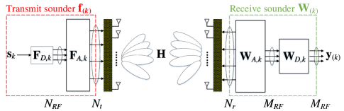
The mmWave MIMO channel sounding model is shown in Fig. 1, where the transmitter and receiver are equipped with and antennas, respectively. There are and RF chains at the transmitter and receiver, respectively. Without loss of generality, we assume is an integer multiple of , and is also an integer multiple of . In the considered mmWave channel sounding framework, one sounding symbol is transmitted over a unit time interval from the transmitter, which is defined as one channel use. It is assumed that the system employs channel uses for channel sounding. The received signal at the th channel use is given by
| (1) |
where is the receive sounder composed of receive analog sounder and receive digital sounder in series, is the transmit sounder composed of transmit analog sounder and transmit digital sounder in series with transmitted sounding signal , and is the noise.
Considering that the transmitted sounding signal is included in , for convenience, we let , which enables us to focus on the design of and . It is worth noting that the analog sounders are constrained to be constant modulus, that is, , and . Without loss of generality, we assume the power of the transmit sounder is one, that is, . The noise is an independent zero mean complex Gaussian vector with covariance matrix . Due to the unit power of transmit sounder, we define the signal-to-noise-ratio (SNR) as .111Here, the SNR is the ratio of transmitted sounder’s power to the noise’s power, which is a common practice in the channel estimation literature [4, 8, 9, 10, 16, 17]. The details of designing the receive and transmit sounders for facilitating the channel estimation will be discussed in Section III.
To model the point-to-point sparse mmWave MIMO channel, we assume there are clusters with , and each constitutes a propagation path. The channel model can be expressed as [18, 19],
| (2) |
where and are array response vectors of the uniform linear arrays (ULAs) at the receiver and transmitter, respectively. We extend it to the channel model with 2D uniform planar arrays (UPAs) in Section IV-C. In particular, and are expressed as
where is the wavelength, is the antenna spacing, and are the angle of arrival (AoA) and angle of departure (AoD) of the th path uniformly distributed in , respectively, and is the complex gain of the th path.
II-B Performance Evaluation of Channel Estimation
To evaluate the channel estimation performance, the achieved spectrum efficiency by utilizing the channel estimate is discussed in the following. Conventionally, the precoder and combiner are designed, based on the estimated , where is the number of transmitted data streams with . Here, when evaluating the channel estimation performance, it is assumed the number of transmitted data streams is equal to the number of dominant paths, i.e., . After the design of precoder and combiner, the received signal for the data transfer is given by
| (4) |
where the signal follows and . It is worth noting that (4) is for data transmission, while (1) is for channel sounding. The spectrum efficiency achieved by and in (4) is defined in [20] as,
| (5) |
where and . In this work, we assume that the precoder and combiner are unitary, such that and . Under this assumption, we have in (5).
It is worth noting that the spectrum efficiency in (5) is invariant to the right rotations of the precoder and combiner, i.e., substituting and into (5), where and are unitary matrices, does not change the spectrum efficiency. Thus, the in (5) is a function of subspaces spanned by the precoder and combiner, i.e., and . Moreover, the highest spectrum efficiency can be achieved when and respectively equal to the row and column subspaces of .
Apart from the spectrum efficiency achieved by the signal model in (4), we consider the effective SNR at the receiver,
| (6) |
The received SNR in (6) has the same rotation invariance property as the spectrum efficiency. In other words, the in (6) is a function of the estimated column and row subspaces. The maximum of the is also achieved when and span the column and row subspaces of , respectively.
Inspired by the definition in (6), in this paper, the accuracy of subspace estimation is defined as the ratio of the power captured by the transceiver matrices [21] and to the power of the channel,
| (7) |
Similarly, the measures for the accuracy of column subspace and row subspace estimation, i.e., and , are respectively defined as the ratio of the power captured by and to the power of the channel in the following,
| (8) | |||||
| (9) |
Moreover, and are also rotation invariant. When the values of or are closed to one, the corresponding or can be treated accurate subspace estimates.
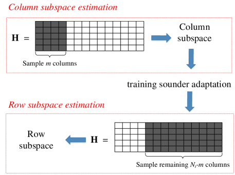
The illustration of the proposed SASE algorithm is shown in Fig. 2. It consists of two stages: one is column subspace estimation and the other is row subspace estimation. In particular, the training sounders of the second stage can be optimized by fully adapting them to the estimated column subspace, which would reduce the number of channel uses and improve the estimation accuracy.
III Sequential and Adaptive Subspace Estimation
III-A Estimate the Column Subspace
In this subsection, we present the design of transmit and receive sounders along with the method for obtaining the column subspace of the mmWave channel. To begin with, the following lemma shows that under the mmWave channel model in (3), the column subspaces of and sub-matrix are equivalent.
Lemma 1
Let be a sub-matrix that selects the first columns of with , where is expressed as
For the mmWave channel model in (3), if all the values of angles and are distinct, the column subspaces of and will be equivalent, i.e., .
Proof:
See Appendix A. ∎∎
Remark 1
Because and are continuous random variables (r.v.s) in , hence, they are distinct almost surely (i.e., with probability ).
Lemma 1 reveals that when , to obtain the column subspace of , it suffices to sample the first columns of , i.e., , which reduces the number of channel uses. However, the mmWave hybrid MIMO architecture can not directly access the entries of due to the analog array constraints. This can be overcome by adopting the technique proposed in [16]. Specifically, to sample the th column of , i.e., , the transmitter needs to construct the transmit sounder , where is the th column of . This is possible due to the fact that any precoder vector can be generated by RF chains [22]. To be more specific, there exists , , and such that ,
where except for , the except for , and .
At the receiver side, we collect the receive sounders of channel uses to form the full-rank matrix,
| (10) |
where , denotes the th receive sounder corresponding to transmit sounder . In order to satisfy the analog constraint where the entries in analog sounders should be constant modulus, we let the matrix in (10) be the discrete Fourier transform (DFT) matrix. Specifically, the analog and digital receive sounders associated with in (10) are expressed as follows
Thus, the received signal under the transmit sounder and receive sounder is expressed as follows
where is the noise vector with . Then we stack the observations of channel uses as ,
| (11) | |||||
where is the effective noise vector after stacking, whose covariance matrix is expressed as,
| (12) |
Because the DFT matrix in (10) satisfies , the following holds
| (15) |
Substituting (15) into (12), we can verify that , and precisely, . Moreover, by denoting , it is straightforward that the entries in are independent, identically distributed (i.i.d.) as . Here, for convenience, we denote where is defined in (11). Then, we apply DFT to the collected observation , and obtain as
| (16) |
where and . Before talking about the noise part in (16), the following lemma is a preliminary which gives the distribution of entries in the product of matrices.
Lemma 2
Given a semi-unitary matrix with , and a random matrix with i.i.d. entries of , the product also has i.i.d. entries with distribution of .
Proof:
See Appendix B. ∎∎
Therefore, considering the noise part in (16), i.e., , where is unitary and has i.i.d. entries, the conclusion of Lemma 2 can be applied, which verifies that the entries of in (16) are i.i.d. as .
Given the expression in (16), the column subspace estimation problem is formulated as,
| (17) |
where one of the optimal solutions of (17) can be obtained by taking the dominant left singular vectors of . Here, the number of paths, , is assumed to be known as a priori. In practice, it is possible to estimate by comparing the singular values of [23]. Because and , there will be singular values of whose magnitudes clearly dominate the other singular values. Alternatively, we can set it to , which is an upper bound on the number of dominant paths such that .222Due to the limited RF chains, the dimension of channel subspaces for data transmission is less than . Thus, if the path number estimate is larger than , we let it be .
Now, we design the receive combiner in (4) for data transmission to approximate the estimated in (17). Specifically, we design the analog combiner and digital combiner at the receiver by solving the following problem
| (18) |
The problem above can be solved by using the OMP algorithm [5] or alternating minimization method [24]. The designed receive combiner is given by with . The methods in [5, 24] have shown to guarantee the near optimal performance, such as . The details of our column subspace estimation algorithm are summarized in Algorithm 1.
In general, is not equal to the column subspace of , i.e., with , due to the noise in (16). To analyze the column subspace accuracy defined in (8), we introduce the theorem [25] below.
Theorem 1 ([25])
Suppose is of rank-, and , where is i.i.d. with zero mean and unit variance (not necessarily Gaussian). Let the compact SVD of be
where , , and . We assume the singular values in are in descending order, i,e, . Similarly, we partition the SVD of as
where , , , , , and . Then, there exists a constant such that
where the expectation is taken over the random noise . In particular, when the noise is i.i.d. , it has .
We have the following proposition for the accuracy of the column subspace estimation in Algorithm 1.
Proposition 1
If the Euclidean distance in (18), then the accuracy of the estimated column subspace matrix obtained from Algorithm 1 is lower bounded as
| (19) |
where is the matrix composed of dominant left singular vectors of . In particular, if , we have
| (20) | |||||
where the is the th largest singular value of .
Proof:
See Appendix C. ∎∎
From (20), the larger the value of is, the more accurate the column subspace estimation. Thus, when more columns are used for the column subspace estimation, the estimated column subspace will be more reliable. In particular, when the noise level is low such that in (20), we have
It means that the column subspace estimation accuracy is linearly related to the value of , i.e., . On the other hand, when the noise level is high such that , the bound in (20) can be written as
At low SNR, the column subspace estimation accuracy is quadratically related to , i.e., .
Remark 2
When the number of paths, , increases, the value of in (20) will decrease, which can be interpreted as follows. When , the entries in can be generally approximated as standard Gaussian r.v.s [26]. Moreover, it has been shown in [27, 28] that the th largest singular value of with high probability. As a result, the accuracy of column subspace estimation will be decreased as increases due to (20) of Proposition 1.
III-B Estimate the Row Subspace
In this subsection, we present how to learn the row subspace by leveraging the estimated column subspace matrix . Because we have already sampled the first columns of in the first stage, we only need to sample the remaining columns to estimate the row subspace as shown in Fig. 2.
At the th channel use of the second stage, we observe the th column of , . To achieve this, we employ the transmit sounder as
| (21) |
For the receive sounder, given the estimated column subspace matrix in the first stage, we just let the receive sounder of the second stage be .333It is worth noting that because the estimated column subspace of the first stage is , thus the dimension for receive sounder of second stage is rather than in (1). It is worth noting is trivially applicable for hybrid precoding architecture since is obtained from (18). Therefore, under the transmit sounder in (21) and receive sounder in (18), the observation at the receiver can be given by
| (22) | |||||
where is the noise vector with . Then, the observations in (22) are packed into a matrix as
| (23) | |||||
where , and .
In addition, given the receive sounder and observations of the first stage in (16), we define as,
| (24) |
Combining (24) and (23) yields expressed as,
| (25) | |||||
where , , , and . Meanwhile, since is semi-unitary and the entries in are i.i.d. with distribution , according to Lemma 2, the entries in are also i.i.d. with distribution .
Now, given the expression in (25), the row subspace estimation problem is formulated as,
where the estimated row subspace matrix is obtained as the dominant right singular vectors of . Similarly, in order to design the precoder in (4) for data transmission, we need to approximate the estimated row subspace matrix under the hybrid precoding architecture. Specifically, we design the analog precoder and digital precoder by solving the following problem
| (26) |
Therefore, the transmit precoder is given by with . Similarly, the method on solving (26) in [5] can guarantee . The details of our row subspace estimation algorithm are shown in Algorithm 2. We have the following proposition about the estimated row subspace accuracy for Algorithm 2.
Proposition 2
Proof:
See Appendix D. ∎∎
Similar as the column subspace estimation, the row subspace accuracy linearly increases with the SNR, i.e., at high SNR, and quadratically increases with SNR, i.e., , at low SNR. Also, the accuracy of row subspace estimation decreases with the number of paths, . As the value of in (28) grows, we can have a more accurate row subspace estimation. Moreover, considering , it is intuitive that the estimated column subspace matrix will affect the value of , and then affect the accuracy of row subspace estimation. Specifically, when , we will have , which attains the maximum. In the following, we further discuss the relationship between and .
With the SVD of , i.e., , we have . Then, the following relationship is true due to the singular value product inequality,
| (29) | |||||
Therefore, is lower bounded by the product of the th largest singular values of and . When the estimation of the column subspace becomes accurate, the will approach to one. As a result, the value of is approximately equal to , resulting in a further enhanced row subspace estimation. The inequality in (29) reveals that the column subspace estimation affects the accuracy of the row subspace estimation.
Given the estimated column subspace in Algorithm 1 and row subspace in Algorithm 2, the following lemma shows the subspace estimation accuracy of the proposed SASE, i.e., defined in (7).
Lemma 3
Proof:
Using the definition of in (7), we have the following expressions,
where the equality holds for and , and the inequality holds based on the singular value product inequality. ∎∎
Lemma 3 tells that the power captured by and is lower bounded by the product of and . These two parts denotes the two stages in the proposed SASE, which are column subspace estimation and row subspace estimation, respectively. Ideally, when and , we have . Nevertheless, the proposed SASE can still achieve nearly optimal . This is because and are close to one according to the bounds provided in (20) and (28), respectively.
III-C Channel Estimation Based on the Estimated Subspaces
In this subsection, we introduce a channel estimation method based on the estimated column subspace and row subspace . Let the channel estimate be expressed as
| (31) |
where . Now, given and , it only needs to obtain in an optimal manner.
Recalling the column subspace estimation in Section III-A and row subspace estimation in Section III-B, the corresponding received signals are expressed as
It is worth noting that the entries in and are both i.i.d with distribution . Based on the expression of in (31), the maximum likelihood estimation of in (31) can be obtained through the following least squares problem,
| (32) |
Before discussing how to solve the problem in (32), for convenience, we define
Using the definitions above, the minimization problem in (32) can be rewritten as
| (33) |
The following lemma provides the solution of problem (33).
Lemma 4
Given the problem below
the optimal solution is given by
| (34) |
Proof:
IV Discussion of Algorithm
In this section, we analyze the complexity of the proposed SASE method in terms of the channel use overhead and computational complexity. Moreover, we discuss the application of the SASE in other channel scenarios.
IV-A Channel Use Overhead
| Algorithms | Number of Channel Uses |
|---|---|
| SASE | |
| MF [11] | |
| SD [10] | |
| Arnoldi [16] | |
| OMP [8] | |
| SBL [9] | |
| ACE [17] |
Considering the channel uses in each stage, the total number of channel uses for the SASE is given by
| (36) |
Therefore, the number of channel uses grows linearly with the channel dimension, i.e., . In particular, when we let , the number of channel uses in (36) will be . Considering that each channel use contributes to observations in the first stage, and observations in the second stage, the total number of the observations is , which is equivalent to the degrees of freedom of - matrix [29].
The numbers of channel uses of the proposed SASE and other benchmarks [8, 9, 17, 10, 11, 16] are compared in Table I. For the angle estimation methods in [8, 9, 17], the number of required channel uses for the OMP [8] and SBL [9] is , where is the number of grids with . The number of channel uses for adaptive channel estimation (ACE) [17] is , where with is the desired angle resolution for the ACE, and is the number of beamforming vectors in each stage of the ACE. For the subspace estimation methods in [10, 11, 16], the numbers of required channel uses for subspace decomposition (SD) [10] and matrix factorization (MF) [11] are , while it requires channel uses where for Arnoldi approach [16]. Because the number of estimated parameters of the angle estimation methods such as OMP, SBL, and ACE, is less than that of the proposed SASE, they require slightly fewer channel uses than SASE. Nevertheless, the proposed SASE consumes fewer channel uses than those of the existing subspace estimation methods [10, 11, 16] as shown in Table I.
IV-B Computational Complexity
For the proposed SASE, the computational complexity of the first stage comes from the SVD of , which is [28]. The complexity of the second stage is dominated by the design of in (18), which is , where denotes the cardinality of an over-complete dictionary. Hence, the overall complexity of the proposed SASE algorithm is . The computational complexities of benchmarks, i.e., the angle estimation methods OMP [8], SBL [9], and ACE [17] along with the subspace estimation methods Arnoldi [16], SD [10], and MF [11] are compared in Table II, where denotes the number of channel uses. For a fair comparison, when comparing the computational complexity, we assume the number of channel uses, , is equal among the benchmarks. As we can see from Table II, the proposed SASE has the lowest computational complexity.
IV-C Extension of SASE
In this subsection, we extend the proposed SASE to the 2D mmWave channel model with UPAs. There are clusters, and each of cluster is composed of rays. For this model, the mmWave channel matrix is expressed as [30, 31, 5]
| (37) |
where represents the complex gain associated with the th path of the th cluster. The and are the receive and transmit array response vectors, where and denote the azimuth and elevation angles of the receiver (transmitter). Specifically, the and are expressed as
where and are the antenna spacing and the wavelength, respectively, and are the antenna indices in the 2D plane.
For the channel model in (37), it is worth noting that the rank of is at most . Using the similar derivations as the proof of Lemma 1, we can verify that when , the sub-matrix satisfies . Therefore, it is possible to sample the first columns of in (37) to obtain column subspace information, and sample the remaining columns to obtain the row subspace information. This means that the proposed SASE can be extended directly to the channel model given in (37).
In summary, the proposed SASE has no strict limitations to be applied to other channel models if the channel matrix experiences sparse propagation and . Moreover, because the proposed SASE is an open-loop framework, it can be easily extended to multiuser MIMO downlink scenarios.
V Simulation Results
In this section, we evaluate the performance of the proposed SASE algorithm by simulation.
V-A Simulation Setup
In the simulation, we consider the numbers of the receive and transmit antennas are , and , respectively, and the numbers of the RF chains at the receiver and transmitter are and , respectively. Without lose of generality, it is assumed that the variance of the complex gain of the th path is . We consider three subspace-based channel estimation methods as the benchmarks, i.e., SD [10] and MF [11], and Arnoldi [16], where SD and MF aim to recover the low-rank mmWave channel matrix, and Arnoldi is to estimate the dominant singular subspaces of the mmWave channel. For a fair comparison, the considered benchmarks are to estimate the subspace rather than the parameters such as the angles of the paths.
V-B Numerical Results
In order to evaluate the subspace accuracy of different methods, we compute the subspace accuracy in (7), column subspace accuracy in (8), and row subspace accuracy in (9) for comparison. We also evaluate the normalized mean squared error (NMSE) and spectrum efficiency. The NMSE is defined as , where denotes the channel estimate. In particular, the channel estimate of the SASE is obtained by the method derived in Section III-C. The spectrum efficiency in (5) is calculated with the combiner and precoder , which are designed according to the precoding design techniques provided in [5] with the obtained channel estimate via channel estimation.
 |
| (a) |
 |
| (b) |
 |
| (c) |
V-B1 Equivalence of Subspace
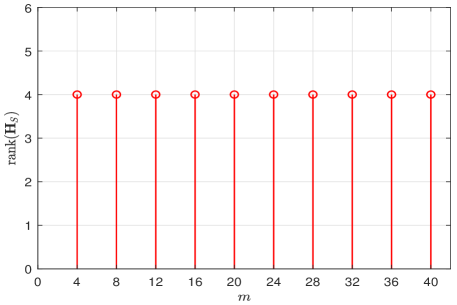
It is worth noting that the column subspace estimation in Section III-A depends on the fact of subspace equivalence between and in (16). We illustrate in Fig. 3 the rank of with different . In this simulation, we set and . It can be seen in Fig. 3 that the rank of is equal to for all the values of , i.e., the rank of is equal to the rank of , for . This validates the fact that .
V-B2 Performance versus Signal-to-Noise Ratio
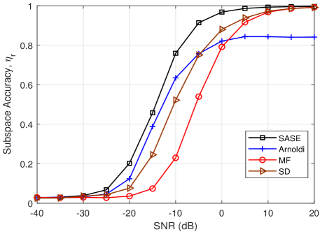
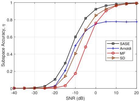
In Fig. 4 and Fig. 5, we compare the performance versus SNR of the proposed SASE algorithm to SD, MF and Arnoldi methods. The number of paths is set as . For a fair comparison, the numbers of channel uses for the benchmarks are kept approximately equal, i.e., .
 |
| (a) |
 |
| (b) |
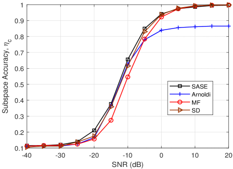
In Fig. 4(a), the column subspace accuracy of the proposed SASE is compared with the benchmarks. As we can see, the SASE and SD methods obtain nearly similar column subspace accuracy, and they outperform over the MF and Arnoldi. It means that sampling the sub-matrix of the channel can provide a robust column subspace estimation. In Fig. 4(b), the row subspace accuracy versus SNR is plotted. We found that the proposed SASE outperforms over the others. It verifies that adapting the receiver sounders to the column subspace can surely improve the accuracy of row subspace estimation. In Fig. 4(c), the subspace accuracy defined in (7) of the proposed SASE is evaluated. As can be seen that the proposed SASE achieves the most accurate subspace estimation over the other methods. For the SASE, MF and SD, the nearly optimal subspace estimation, i.e., , can be achieved in the high SNR region (). Since the performance of the Arnoldi highly depends on the number of available channel uses, its accuracy is degraded and saturated at high SNR due to the limited channel uses (). Thus, the ideal performance of the Arnoldi relies on a large number of channel uses or enough RF chains [16].
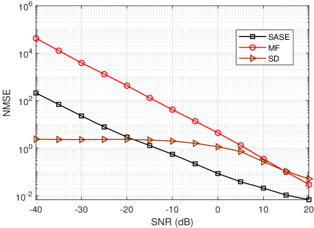
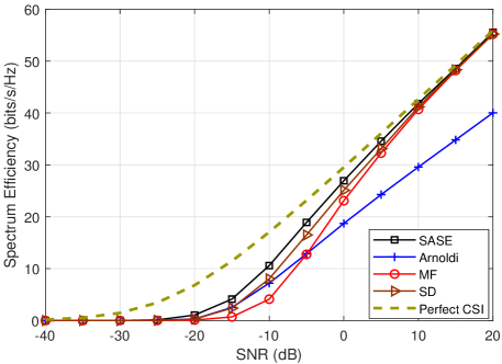
In Fig. 5(a), the NMSE of the proposed SASE is decreased as the SNR increases. It has similar characteristis as that of the MF, but has much lower value. The NMSE of the SD is almost constant in the low SNR region and decreases in higher SNR region. Overall, the SASE outperforms the SD when . In Fig. 5(b), the spectral efficiency of the SASE is plotted. The curve for perfect CSI with fully digital precoding is plotted for comparison. The proposed SASE achieves the nearly optimal spectrum efficiency among all the methods. It is observed that the spectrum efficiency of the SASE has a different trend from the NMSE in Fig. 5(a), while it has similar characteristic as the subspace accuracy in Fig. 4(c). The evaluation validates the effectiveness of the SASE in channel estimation to provide good spectrum efficiency.
 |
| (a) |
 |
| (b) |
V-B3 Performance versus Number of Channel Uses
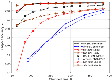
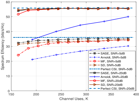
In Fig. 6, we show the channel estimation performance of the SASE for different numbers of channel uses. The simulation setting is . The value of in (36) is in the set of . Accordingly, the set of the numbers of channel uses is .
 |
| (a) |
 |
| (b) |
Fig. 6(a) shows the subspace estimation performance versus the number of channel uses. As the number of channel uses increases, the subspace accuracy of all the methods is increased monotonically. It is worth noting that when (), the subspace accuracy of the SASE is slightly lower than that of the SD. This is because there are only columns sampled for column subspace estimation that affects the column subspace accuracy of the SASE slightly. Nevertheless, when , i.e., , the SASE obtains the most accurate subspace estimation, i.e., , among all the methods. In particular, when the SNR is moderate, i.e., SNRdB, the SASE clearly outperforms over the other methods. This means that the SASE requires less channel uses to provide a robust subspace estimation.
Fig. 6(b) shows the spectrum efficiency versus the number of channel uses. The curve for perfect CSI with fully digital precoding is also plotted for comparison. Again, the SASE achieves nearly optimal spectrum efficiency compared to the other methods. The performance gap between the SASE and the other methods are more noticeable at SNRdB. In particular, as seen in the figure, when the number of channel uses, , the performance gap between the SASE and perfect curve at SNRdB is less than bits/s/Hz.
V-B4 Performance versus Number of Paths
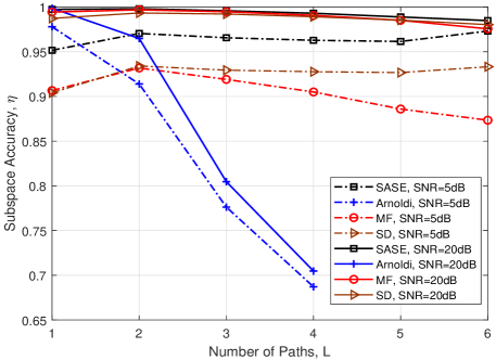
In Fig. 7, we evaluate the estimation performance of the SASE for different numbers of paths, . The number of channel uses is and . Due to the limited number of channel uses, the Anorldi method can not perform the channel estimation for . Thus, we only show the performance of the Arnoldi for .
In Fig. 7(a), the subspace accuracy of different methods versus number of paths, , is illustrated. As we can see, the SASE, SD and MF achieve a more accurate subspace estimation compared to the Arnoldi. It is seen that the Arnoldi has a sharp decrease in the accuracy for . It means that the Arnoldi can provide a good channel estimate only for with the use of channel uses. When SNRdB, the SASE outperforms over the other methods. When the SNR is high, i.e., SNRdB, for the proposed SASE, the subspace accuracy decreases slightly with the number of paths, , which verifies our discussion about the effect of in Remark 2 of Section III.
 |
| (a) |
 |
| (b) |
 |
| (c) |
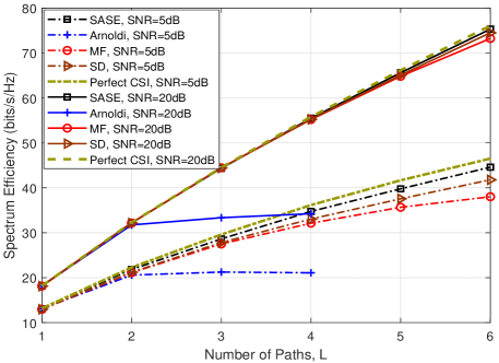
In Fig. 7(b), the spectrum efficiency versus number of paths, , is shown. Apart from the Arnoldi, the spectrum efficiency achieved by the SASE, MF and SD increases with the number of paths. When the SNR is high, i.e., SNRdB, the SASE, MF and SD can achieve nearly optimal performance. When the SNR is moderate, i.e., SNRdB, the proposed SASE achieves the highest spectrum efficiency among all the methods. Moreover, for the SASE, MF and SD, their performance gaps with the curve of perfect CSI is getting wider as increases. Nevertheless, the spectrum efficiency of the SASE is more closer than the other methods, which implies that the SASE can leverage the property of limited number of paths in mmWave channels more effectively than the other methods.
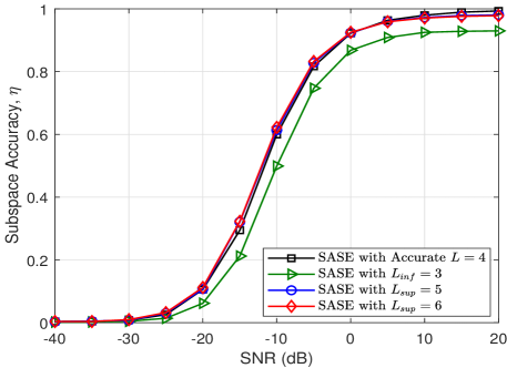
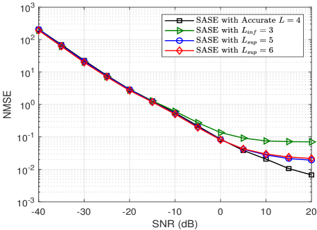
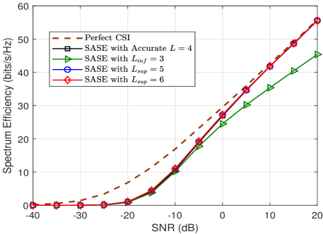
V-B5 Performance versus Inaccurate Path information
Thus far, in the previous simulations, we have assumed the number of paths, , is known a priori. In Fig. 8, we evaluate the performance of the SASE under the situation that the accurate path information is not available. As discussed in Section III-A, we utilize the upper bound of the number of paths for simplicity, where we let while .444If the with is utilized for SASE, the estimated subspaces will be and . For a fair comparison, we choose the dominant modes in and when evaluating the performance. For a clear illustration, we also evaluate the performance of proposed SASE by using the lower bound of number of paths, i.e., . As can be seen in Fig. 8, compared to the case of , using the upper bound for SASE achieves a similar performance as the accurate path information of . In particular, it is noted in Fig. 8(a) and Fig. 8(b) that the estimation performance of is slightly worse than that of accurate path information when SNR is high, while it is marginally better when SNR is low. This is because using inaccurate path information with does not affect the column subspace estimation, but according to Proposition 2, it provides worse row subspace estimation at high SNR and more accurate row subspace estimation at low SNR.555It is worth noting that if is utilized for SASE, according to Proposition 2, the row subspace accuracy is bounded as . The statements can be verified easily through analyzing this row subspace accuracy bound. Nevertheless, in overall, the performance of proposed SASE is not sensitive to the inaccurate path number.
VI Conclusion
In this paper, we formulate the mmWave channel estimation as a subspace estimation problem and propose the SASE algorithm. In the SASE algorithm, the channel estimation task is divided into two stages: the first stage is to obtain the column channel subspace, and in the second stage, based on the acquired column subspace, the row subspace is estimated with optimized training signals. By estimating the column and row subspaces sequentially, the computational complexity of the proposed SASE was reduced substantially to with . It was analyzed that channel uses are sufficient to guarantee subspace estimation accuracy of the proposed SASE. By simulation, the proposed SASE has better subspace accuracy, lower NMSE, and higher spectrum efficiency than those of the existing subspace methods for practical SNRs.
Appendix A Proof of Lemma 1
From the mmWave channel model in (3), when the angles and are distinct,
which holds due to the fact that and are both Vandermonde matrices. Then, can be expressed as
Combining the rank inequality of matrix product and the following lower bound,
yields . Therefore, in order to show , namely, , it suffices to show that . Considering that is a Vandermonde matrix, it has . This completes the proof. ∎
Appendix B Proof of Lemma 2
It is trivial that the entries in follow the identical distribution of . Therefore, it remains to show that all the entries in are independent. Because of the typical property of Gaussian distribution, it suffices to prove that they are uncorrelated. For any or , the following holds,
Therefore, the entries in are uncorrelated and thus independent, which concludes the proof. ∎
Appendix C Proof of Proposition 1
Appendix D Proof of Proposition 2
Recall that the row subspace matrix is given by the right singular matrix of in (25), and the elements in are i.i.d. with each entry being according to Lemma 2. Thus, Theorem 1 is applied, which gives
| (40) |
Then, based on the subspace accuracy metric in (9), it has
| (41) | |||||
Thus, the inequality (27) is proved. Moreover, under the condition , taking expectation of the squares of both sides in (41) yields
where the inequality holds from (40). This concludes the proof for the row estimation accuracy bound in (28). ∎
References
- [1] T. S. Rappaport, S. Sun, R. Mayzus, H. Zhao, Y. Azar, K. Wang, G. N. Wong, J. K. Schulz, M. Samimi, and F. Gutierrez, “Millimeter wave mobile communications for 5G cellular: It will work!” IEEE Access, vol. 1, pp. 335–349, 2013.
- [2] R. W. Heath, N. González-Prelcic, S. Rangan, W. Roh, and A. M. Sayeed, “An overview of signal processing techniques for millimeter wave MIMO systems,” IEEE J. Sel. Top. Signal Process., vol. 10, no. 3, pp. 436–453, April 2016.
- [3] E. Torkildson, U. Madhow, and M. Rodwell, “Indoor millimeter wave MIMO: Feasibility and performance,” IEEE Trans. Wireless Commun., vol. 10, no. 12, pp. 4150–4160, 2011.
- [4] S. Hur, T. Kim, D. J. Love, J. V. Krogmeier, T. A. Thomas, and A. Ghosh, “Millimeter wave beamforming for wireless backhaul and access in small cell networks,” IEEE Trans. Commun., vol. 61, no. 10, pp. 4391–4403, 2013.
- [5] O. El Ayach, S. Rajagopal, S. Abu-Surra, Z. Pi, and R. W. Heath, “Spatially sparse precoding in millimeter wave MIMO systems,” IEEE Trans. Wireless Commun., vol. 13, no. 3, pp. 1499–1513, 2014.
- [6] J. Wang, Z. Lan, C. Pyo, T. Baykas, C. Sum, M. A. Rahman, J. Gao, R. Funada, F. Kojima, H. Harada, and S. Kato, “Beam codebook based beamforming protocol for multi-Gbps millimeter-wave WPAN systems,” IEEE J. Sel. Areas Commun., vol. 27, no. 8, pp. 1390–1399, Oct 2009.
- [7] O. E. Ayach, R. W. Heath, S. Abu-Surra, S. Rajagopal, and Z. Pi, “The capacity optimality of beam steering in large millimeter wave mimo systems,” in 2012 IEEE 13th International Workshop on Signal Processing Advances in Wireless Communications (SPAWC), June 2012, pp. 100–104.
- [8] J. Lee, G. T. Gil, and Y. H. Lee, “Channel estimation via orthogonal matching pursuit for hybrid MIMO systems in millimeter wave communications,” IEEE Trans. Commun., vol. 64, no. 6, pp. 2370–2386, June 2016.
- [9] S. Srivastava, A. Mishra, A. Rajoriya, A. K. Jagannatham, and G. Ascheid, “Quasi-static and time-selective channel estimation for block-sparse millimeter wave hybrid MIMO systems: Sparse bayesian learning (sbl) based approaches,” IEEE Trans. Signal Process., vol. 67, no. 5, pp. 1251–1266, March 2019.
- [10] W. Zhang, T. Kim, D. J. Love, and E. Perrins, “Leveraging the restricted isometry property: Improved low-rank subspace decomposition for hybrid millimeter-wave systems,” IEEE Trans. Commun., vol. 66, no. 11, pp. 5814–5827, Nov 2018.
- [11] P. Jain, P. Netrapalli, and S. Sanghavi, “Low-rank matrix completion using alternating minimization,” in Proceedings of the Forty-fifth Annual ACM Symposium on Theory of Computing, ser. STOC ’13. New York, NY, USA: ACM, 2013, pp. 665–674.
- [12] B. Recht, M. Fazel, and P. A. Parrilo, “Guaranteed minimum-rank solutions of linear matrix equations via nuclear norm minimization,” SIAM Rev., vol. 52, no. 3, pp. 471–501, 2010.
- [13] X. Li, J. Fang, H. Li, and P. Wang, “Millimeter wave channel estimation via exploiting joint sparse and low-rank structures,” IEEE Trans. Wireless Commun., vol. 17, no. 2, pp. 1123–1133, Feb 2018.
- [14] W. Zhang, T. Kim, G. Xiong, and S.-H. Leung, “Leveraging subspace information for low-rank matrix reconstruction,” Signal Process., vol. 163, pp. 123 – 131, 2019.
- [15] W. Zhang, T. Kim, and D. Love, “Sparse subspace decomposition for millimeter wave MIMO channel estimation,” in 2016 IEEE Global Communications Conference: Signal Processing for Communications (Globecom2016 SPC), Washington, USA, Dec. 2016.
- [16] H. Ghauch, T. Kim, M. Bengtsson, and M. Skoglund, “Subspace estimation and decomposition for large millimeter-wave MIMO systems,” IEEE J. Sel. Top. Signal Process., vol. 10, no. 3, pp. 528–542, April 2016.
- [17] A. Alkhateeb, O. El Ayach, G. Leus, and R. W. Heath, “Channel estimation and hybrid precoding for millimeter wave cellular systems,” IEEE J. Sel. Top. Signal Process., vol. 8, no. 5, pp. 831–846, Oct 2014.
- [18] R. Heath, N. Gonzalez-Prelcic, S. Rangan, W. Roh, and A. Sayeed, “An overview of signal processing techniques for millimeter wave MIMO systems,” IEEE J. Sel. Top. Signal Process., vol. PP, no. 99, pp. 1–1, 2016.
- [19] J. Brady, N. Behdad, and A. M. Sayeed, “Beamspace MIMO for millimeter-wave communications: System architecture, modeling, analysis, and measurements,” IEEE Trans. Antennas Propag., vol. 61, no. 7, pp. 3814–3827, 2013.
- [20] A. Goldsmith, S. A. Jafar, N. Jindal, and S. Vishwanath, “Capacity limits of MIMO channels,” IEEE J. Sel. Areas Commun., vol. 21, no. 5, pp. 684–702, June 2003.
- [21] S. Haghighatshoar and G. Caire, “Massive MIMO channel subspace estimation from low-dimensional projections,” IEEE Trans. Signal Process., vol. 65, no. 2, pp. 303–318, Jan 2017.
- [22] X. Zhang, A. F. Molisch, and S.-Y. Kung, “Variable-phase-shift-based RF-baseband codesign for MIMO antenna selection,” IEEE Trans. Signal Process., vol. 53, no. 11, pp. 4091–4103, Nov 2005.
- [23] N. El Karoui, “Tracy–widom limit for the largest eigenvalue of a large class of complex sample covariance matrices,” Ann. Probab., vol. 35, no. 2, pp. 663–714, 03 2007.
- [24] X. Yu, J. C. Shen, J. Zhang, and K. B. Letaief, “Alternating minimization algorithms for hybrid precoding in millimeter wave MIMO systems,” IEEE J. Sel. Top. Signal Process., vol. 10, no. 3, pp. 485–500, April 2016.
- [25] T. T. Cai and A. Zhang, “Rate-optimal perturbation bounds for singular subspaces with applications to high-dimensional statistics,” Ann. Statist., vol. 46, no. 1, pp. 60–89, 02 2018.
- [26] R. Durrett, Probability: theory and examples. Cambridge University Press, 2010.
- [27] F. Wei, “Upper bound for intermediate singular values of random matrices,” Journal of Mathematical Analysis and Applications, vol. 445, no. 2, pp. 1530–1547, 2017.
- [28] Y. Dagan, G. Kur, and O. Shamir, “Space lower bounds for linear prediction in the streaming model,” in Proceedings of the Thirty-Second Conference on Learning Theory, ser. Proceedings of Machine Learning Research, A. Beygelzimer and D. Hsu, Eds., vol. 99. Phoenix, USA: PMLR, 25–28 Jun 2019, pp. 929–954.
- [29] G. Golub and C. Van Loan, Matrix Computations, ser. Johns Hopkins Studies in the Mathematical Sciences. Johns Hopkins University Press, 2013.
- [30] T. Bai, A. Alkhateeb, and R. W. Heath, “Coverage and capacity of millimeter-wave cellular networks,” IEEE Commun. Mag., vol. 52, no. 9, pp. 70–77, Sep. 2014.
- [31] Z. Pi and F. Khan, “An introduction to millimeter-wave mobile broadband systems,” IEEE Commun. Mag., vol. 49, no. 6, pp. 101–107, June 2011.