This paper was converted on www.awesomepapers.org from LaTeX by an anonymous user.
Want to know more? Visit the Converter page.

A Shape Optimization Problem Constrained with the Stokes Equations to Address Maximization of Vortices

Abstract.

We study an optimization problem that aims to determine the shape of an obstacle that is submerged in a fluid governed by the Stokes equations. The mentioned flow takes place in a channel, which motivated the imposition of a Poiseuille-like input function on one end and a do-nothing boundary condition on the other. The maximization of the vorticity is addressed by the L2L^{2}-norm of the curl and the det-grad measure of the fluid. We impose a Tikhonov regularization in the form of a perimeter functional and a volume constraint to address the possibility of topological change. Having been able to establish the existence of an optimal shape, the first order necessary condition was formulated by utilizing the so-called rearrangement method. Finally, numerical examples are presented by utilizing a finite element method on the governing states, and a gradient descent method for the deformation of the domain. On the said gradient descent method, we use two approaches to address the volume constraint: one is by utilizing the augmented Lagrangian method; and the other one is by utilizing a class of divergence-free deformation fields.

Key words and phrases:
Shape optimization, Stokes equations, augmented Lagrangian, Rearrangment method.
1991 Mathematics Subject Classification:
Primary: 49Q10,76D55, 35Q93; Secondary: 76U99
This work is supported by JSPS KAKENHI Grant Numbers JP18H01135, JP20H01823, JP20KK0058 and JP21H04431, and JST CREST Grant Number JPMJCR2014 for HN; and by the Japanese Government (MEXT) Scholarship for JSS
Corresponding author: john.simon@stu.kanazawa-u.ac.jp

John Sebastian H. Simon

Graduate School of Natural Science and Technology

Kanazawa University

Kanazawa 920-1192, Japan

Hirofumi Notsu

Faculty of Mathematics and Physics

Kanazawa University

Kanazawa 920-1192, Japan


Introduction

The study of fluid dynamics is among the most active areas in mathematics, physics, engineering, and most recently in information theory [13]. An interesting area in this field is the study of turbulent flows and on controlling the emergence of such phenomena [7, 30, 10].

Even though turbulence represents chaos, harnessing it in a controlled manner can be useful, for instance, in optimal mixing problems. Among these studies is [8] where an optimal stirring strategy to maximize mixing is studied, while in [24] the authors studied the best type of input functions that will provide a better mixing in the fluid.

Recently, Goto, K. et.al.[13] utilized the generation of vortices in the fluid for information processing tasks. In the said literature, the authors found out that the length of the twin-vortex affects the memory capacity in the context of physical reservoir computing.

For these reasons, the current paper is dedicated to studying a shape optimization problem intended to maximize the turbulence of a flow governed by the two-dimensional Stokes equations. Here, the shape of an obstacle submerged in a fluid – that flows through a channel – is determined to maximize vorticity. Furthermore, the vorticity is quantified in two ways: one is by the curl of the velocity of the fluid; and the other is by rewarding the unfolding of complex eigenvalues of the gradient tensor of the velocity field.

To be precise, our goal is to study the following shape optimization problem

min{𝒢(𝐮,Ω);|Ω|=m,ΩD},\min\{\mathcal{G}({\operatorname{\boldsymbol{u}}},\Omega);|\Omega|=m,\Omega\subset D\}, (1)

where DD is a hold-all domain which is assumed to be a fixed bounded connected domain in 2\mathbb{R}^{2}, ΩD\Omega\subset D is an open bounded domain, 𝒢(𝐮,Ω):=J(𝐮,Ω)+αP(Ω),\mathcal{G}({\operatorname{\boldsymbol{u}}},\Omega):=J({\operatorname{\boldsymbol{u}}},\Omega)+\alpha P(\Omega), JJ and PP are vortex and perimeter functionals given by

J(𝐮,Ω)=Ωγ12|×𝐮|2+γ2h(det(𝐮))dx,P(Ω)=Γfds,J({\operatorname{\boldsymbol{u}}},\Omega)=-\int_{\Omega}\frac{\gamma_{1}}{2}|\nabla\times{\operatorname{\boldsymbol{u}}}|^{2}+\gamma_{2}h(\mathrm{det}(\nabla{\operatorname{\boldsymbol{u}}}))\operatorname*{d\!}x,\ P(\Omega)=\int_{\Gamma_{\rm f}}\operatorname*{d\!}s,

hh is such that

h(t)={0if t0,t3/(t2+1)if t>0,h(t)=\left\{\begin{matrix}0&\text{if }t\leq 0,\\ t^{3}/(t^{2}+1)&\text{if }t>0,\end{matrix}\right.

|Ω|:=Ωdx|\Omega|:=\int_{\Omega}\operatorname*{d\!}x, and α,γ1,γ2\alpha,\gamma_{1},\gamma_{2} and mm are positive constants. Here, 𝐮{\operatorname{\boldsymbol{u}}} is the velocity field governed by a fluid flowing through a channel with an obstacle (see Figure 1 for reference). The flow of the fluid is reinforced by a divergence-free input function 𝐠\operatorname{\boldsymbol{g}} on the left end of the channel, which is an inflow boundary denoted by Γin\Gamma_{\rm{in}}, whilst an outflow boundary condition is imposed to the fluid on the right end of the channel denoted by Γout\Gamma_{\rm{out}}. The boundary Γf\Gamma_{\rm f} is the free surface and is the boundary of the submerged obstacle in the fluid. The remaining boundaries of the channel are wall boundaries denoted by Γw\Gamma_{\rm{w}}, upon which – together with the obstacle boundary Γf\Gamma_{\rm f} – a no-slip boundary condition is imposed on the fluid. We refer the reader to [11, 15, 21, 25, 33] for shape optimization problems involving fluids among others.

Γin\Gamma_{\rm{in}}Γf\Gamma_{\rm{f}}Γout\Gamma_{\rm{out}}Γw\Gamma_{\rm{w}}Γw\Gamma_{\rm{w}}Ω{\Omega}
Figure 1. Set up of the domain.

We also point out that usually, the curl ×𝐮\nabla\times{\operatorname{\boldsymbol{u}}} is enough to quantify the vorticity of the fluid. However, as pointed out by Kasumba, K. and Kunisch, K. in [23], the magnitude of such quantity may still be high on laminar flows. As such, on the same literature the authors proposed the second term in the vortex functional for the quantification of rotation of fluids. The impetus is that the rotational cores of fluids mostly occur near regions where the eigenvalues of 𝐮\nabla{\operatorname{\boldsymbol{u}}} are complex [4, 19, 22], and that the eigenvalues are complex when det𝐮>0\mathrm{det}\nabla{\operatorname{\boldsymbol{u}}}>0.

Convention: When we talk about a domain Ω\Omega, we always consider it having the boundary Ω=Γ¯inΓ¯wΓ¯outΓ¯f\partial\Omega=\overline{\Gamma}_{\rm in}\cup\overline{\Gamma}_{\rm w}\cup\overline{\Gamma}_{\rm out}\cup\overline{\Gamma}_{\rm f} with meas(ΓiΓj)=0\mathrm{meas}(\Gamma_{i}\cap\Gamma_{j})=0 for i,j{in,w,out,f},iji,j\in\{{\rm in,w,out,f}\},i\neq j, and that dist(Ω\Γf,Γf)>0\mathrm{dist}(\partial\Omega\backslash\Gamma_{\rm f},\Gamma_{\rm f})>0.

One of the challenges in this problem is the non-convexity of the functional JJ, which leads into the possible non-existence of solutions for the shape optimization problem. Fortunately, we will be able to show later on that the functional JJ is continuous with respect to domain variations. Furthermore, the Tikhonov regularization in the form of the perimeter functional PP is taken into consideration to circumvent the issue of possible topological changes of the domain.

Meanwhile, for the equality constraint |Ω|=m|\Omega|=m, we note that the use of an augmented Lagrangian generates smoother solutions as compared to the common Lagrangian. This is due to the regularizing effect of the quadratic augmentation. As a further consequence, this quadratic term also acts as a penalizing term for the violation of the equality constraint. Aside from the augmented Lagrangian, we also propose an analogue of the H1H^{1}-gradient method that satisfies the incompressibility condition to preserve the volume on each iterate of the gradient-descent method.

This paper is organized as follows: in the next section, the system that governs the fluid and the functional spaces to be used for the analysis will be introduced. The variational formulation of the governing system and the existence of its solution will also be shown in the next section. Section 2 is dedicated to the analysis of the existence of an optimal shape. Here, we employ the LL^{\infty}-topology of characteristic functions for convergence of deformed domains, to ensure the volume preservation.

We shall derive the necessary condition for the optimization problem in Section 3. This is done by investigating the sensitivity of the objective functional 𝒢\mathcal{G} with respect to shape variations. In particular, the shape variations are induced by the velocity method [34], and the shape sensitivity is analyzed using the rearrangement method which was formalized by Ito, K., Kunisch, K., and Peichl, G. in [20]. In Section 4, we provide numerical algorithms through the help of the necessary conditions formulated in Section 3, and provide some illustrations of how these algorithms are implemented. To objectively observe the effects of the final shapes to fluid vortices, we look at the generation of twin-vortices in a dynamic nonlinear fluid flow. Finally, we draw conclusions and possible problems on the last section.

1. Preliminaries

1.1. Governing equations and necessary functional spaces

Let ΩD\Omega\subset D be open, bounded and of class C1,1C^{1,1}, the motion of the fluid is described by its velocity 𝐮{\operatorname{\boldsymbol{u}}} and pressure pp which satisfies the stationary Stokes equations given by:

{νΔ𝐮+p=𝐟 in Ω,div𝐮=0 in Ω,𝐮=𝐠 on Γin,𝐮=0 on ΓfΓw,p𝐧+ν𝐧𝐮=0 on Γout,\displaystyle\left\{\begin{aligned} \,-\nu\Delta{\operatorname{\boldsymbol{u}}}+\nabla p&=\operatorname{\boldsymbol{f}}&&\text{ in }\Omega,\\ \,\operatorname*{div}{\operatorname{\boldsymbol{u}}}&=0&&\text{ in }\Omega,\\ \,{\operatorname{\boldsymbol{u}}}&=\operatorname{\boldsymbol{g}}&&\text{ on }\Gamma_{\rm in},\\ \,{\operatorname{\boldsymbol{u}}}&=0&&\text{ on }\Gamma_{\rm{f}}\cup\Gamma_{\rm w},\\ \,-p\operatorname{\boldsymbol{n}}+\nu\partial_{\operatorname{\boldsymbol{n}}\!}{\operatorname{\boldsymbol{u}}}&=0&&\text{ on }\Gamma_{\rm out},\end{aligned}\right. (2)

where ν>0\nu>0 is a constant, 𝐟\operatorname{\boldsymbol{f}} is an external force, 𝐠\operatorname{\boldsymbol{g}} is a divergence-free input function acting on the boundary Γin\Gamma_{\rm in}, 𝐧\operatorname{\boldsymbol{n}} is the outward unit normal vector on Ω\partial\Omega, and 𝐧:=𝐧\partial_{\operatorname{\boldsymbol{n}}}:=\operatorname{\boldsymbol{n}}\cdot\nabla is the 𝐧\operatorname{\boldsymbol{n}}-directional derivative on Ω\partial\Omega. The condition 𝐮=0{\operatorname{\boldsymbol{u}}}=0 on ΓfΓw\Gamma_{\rm{f}}\cup\Gamma_{\rm w} corresponds to no-slip boundary condition, while the Neumann condition on Γout\Gamma_{\rm out} is the so-called do-nothing boundary condition.

The analysis will take place in the Sobolev spaces Wk,p(D)W^{k,p}(D) for D2D\subset\mathbb{R}^{2}, k0k\geq 0 and p1p\geq 1. Note that if p=2p=2, then Hk(D)=Wk,2(D)H^{k}(D)=W^{k,2}(D) and H0(D)=L2(D)H^{0}(D)=L^{2}(D). For any domain Ω2\Omega\subset\mathbb{R}^{2}, we define

𝒲(Ω)={𝝋C(Ω)2:𝝋=0 on a neighborhood of Γ0:=Ω\Γout}.\mathcal{W}(\Omega)=\{\boldsymbol{\varphi}\in C^{\infty}(\Omega)^{2}:\boldsymbol{\varphi}=0\text{ on a neighborhood of }\Gamma_{0}:=\partial\Omega\backslash\Gamma_{\rm out}\}.

We denote by 𝐇Γ0r(Ω)\operatorname{\mathbf{H}}_{\Gamma_{0}}^{r}(\Omega) the closure of 𝒲(Ω)\mathcal{W}(\Omega) with respect to the space Hr(Ω)2H^{r}(\Omega)^{2}.

We also consider the following bilinear forms a(,)Ω:H2(Ω)2×H2(Ω)2a(\cdot,\cdot)_{\Omega}:H^{2}(\Omega)^{2}\times H^{2}(\Omega)^{2}\to\mathbb{R} and b(,)Ω:H2(Ω)2×L2(Ω)b(\cdot,\cdot)_{\Omega}:H^{2}(\Omega)^{2}\times L^{2}(\Omega)\to\mathbb{R} defined by

a(𝐮,𝐯)Ω=Ω𝐮:𝐯dx,b(𝐯,q)Ω=Ωqdiv𝐯dx.\displaystyle a({\operatorname{\boldsymbol{u}}},\operatorname{\boldsymbol{v}})_{\Omega}=\int_{\Omega}\nabla{\operatorname{\boldsymbol{u}}}:\nabla\operatorname{\boldsymbol{v}}\operatorname*{d\!}x,\ b(\operatorname{\boldsymbol{v}},q)_{\Omega}=-\int_{\Omega}q\operatorname{\mathrm{div}}\operatorname{\boldsymbol{v}}\operatorname*{d\!}x.

Furthermore, for any measurable set 𝒟d\mathcal{D}\subset\mathbb{R}^{d} (d=1,2d=1,2) we shall denote (,)𝒟(\cdot,\cdot)_{\mathcal{D}} as the L2(𝒟)L^{2}(\mathcal{D}), L2(𝒟)2L^{2}(\mathcal{D})^{2} or L2(𝒟)2×2L^{2}(\mathcal{D})^{2\times 2} inner product.

1.2. Weak formulation and existence of solutions

Let 𝐠H2(D)2\operatorname{\boldsymbol{g}}\in H^{2}(D)^{2} satisfy the following properties:

{div𝐠=0 in Ω;𝐠=0 on ΓfΓwall;Γout𝐠𝐧ds=Γin𝐠𝐧ds0,\displaystyle\left\{\begin{aligned} &\operatorname*{div}\operatorname{\boldsymbol{g}}=0\text{ in }\Omega;\quad\operatorname{\boldsymbol{g}}=0\text{ on }\Gamma_{\rm f}\cup\Gamma_{\rm wall};\\ &\int_{\Gamma_{\rm out}}\operatorname{\boldsymbol{g}}\cdot\operatorname{\boldsymbol{n}}\operatorname*{d\!}s=-\int_{\Gamma_{\rm in}}\operatorname{\boldsymbol{g}}\cdot\operatorname{\boldsymbol{n}}\operatorname*{d\!}s\geq 0,\end{aligned}\right. (3)

and 𝐟L2(D)2\operatorname{\boldsymbol{f}}\in L^{2}(D)^{2}. The existence of the function 𝐠H2(D)2\operatorname{\boldsymbol{g}}\in H^{2}(D)^{2} that satisfies (3), can be easily established by utilizing for instance [12, Lemma 2.2].

By letting 𝐮~=𝐮𝐠\tilde{\operatorname{\boldsymbol{u}}}={\operatorname{\boldsymbol{u}}}-\operatorname{\boldsymbol{g}}, we consider the variational form of the state equation (2) given by: For a given domain Ω\Omega, find (𝐮~,p)𝐇Γ01(Ω)×L2(Ω)(\tilde{\operatorname{\boldsymbol{u}}},p)\in\operatorname{\mathbf{H}}_{\Gamma_{0}}^{1}(\Omega)\times L^{2}(\Omega) that satisfies, for any (𝝋,q)𝐇Γ01(Ω)×L2(Ω)(\operatorname{\boldsymbol{\varphi}},q)\in\operatorname{\mathbf{H}}_{\Gamma_{0}}^{1}(\Omega)\times L^{2}(\Omega), the following equations

{νa(𝐮~,𝝋)Ω+b(𝝋,p)Ω=(𝐟,𝝋)Ων(𝐠,𝝋)Ωb(𝐮~,q)Ω=0.\left\{\begin{aligned} \nu a(\tilde{\operatorname{\boldsymbol{u}}},\operatorname{\boldsymbol{\varphi}})_{\Omega}+b(\operatorname{\boldsymbol{\varphi}},p)_{\Omega}&=(\operatorname{\boldsymbol{f}},\operatorname{\boldsymbol{\varphi}})_{\Omega}-\nu(\nabla\operatorname{\boldsymbol{g}},\nabla\operatorname{\boldsymbol{\varphi}})_{\Omega}\\ b(\tilde{\operatorname{\boldsymbol{u}}},q)_{\Omega}&=0.\end{aligned}\right. (4)

Any pair (𝐮~,p)𝐇Γ01(Ω)×L2(Ω)(\tilde{\operatorname{\boldsymbol{u}}},p)\in\operatorname{\mathbf{H}}_{\Gamma_{0}}^{1}(\Omega)\times L^{2}(\Omega) that solves the variational equation (4) is said to be a weak solution to the Stokes equation (2). The existence of the solution 𝐮~\tilde{\operatorname{\boldsymbol{u}}}, is summarized below.

Theorem 1.1.

Let Ω\Omega be of class C1,1,C^{1,1}, 𝐟L2(D)2\operatorname{\boldsymbol{f}}\in L^{2}(D)^{2}, and 𝐠H2(D)2\operatorname{\boldsymbol{g}}\in H^{2}(D)^{2} satisfy (3). The solution (𝐮~,p)𝐇Γ01(Ω)×L2(Ω)(\tilde{\operatorname{\boldsymbol{u}}},p)\in\operatorname{\mathbf{H}}_{\Gamma_{0}}^{1}(\Omega)\times L^{2}(\Omega) to the variational problem (4) exists such that

𝐮~𝐇Γ01(Ω)+pL2(Ω)c(𝐟L2(Ω)2+𝐠H1(Ω)2).\|\tilde{\operatorname{\boldsymbol{u}}}\|_{\operatorname{\mathbf{H}}_{\Gamma_{0}}^{1}(\Omega)}+\|p\|_{L^{2}(\Omega)}\leq c(\|\operatorname{\boldsymbol{f}}\|_{L^{2}(\Omega)^{2}}+\|\operatorname{\boldsymbol{g}}\|_{H^{1}(\Omega)^{2}}). (5)

for some constant c>0c>0.

The proof of the theorem above can be done by utilizing the fact that the operator a(,)Ωa(\cdot,\cdot)_{\Omega} is coercive, b(,)Ωb(\cdot,\cdot)_{\Omega} satisfies the inf-sup condition [12], and that the right hand side of the first equation of (4) can be seen as an action of an element of 𝐇1(Ω)\operatorname{\mathbf{H}}^{-1}(\Omega).

Remark 1.

(i) The energy estimate can be extended to the hold-all domain DD, i.e.,

𝐮~𝐇Γ01(Ω)+pL2(Ω)c(𝐟L2(D)2+𝐠H1(D)2),\|\tilde{\operatorname{\boldsymbol{u}}}\|_{\operatorname{\mathbf{H}}_{\Gamma_{0}}^{1}(\Omega)}+\|p\|_{L^{2}(\Omega)}\leq c(\|\operatorname{\boldsymbol{f}}\|_{L^{2}(D)^{2}}+\|\operatorname{\boldsymbol{g}}\|_{H^{1}(D)^{2}}),

where c>0c>0 is dependent on DD but not on Ω\Omega. (ii) As expected, a more regular domain yields a more regular solution. In particular, if Ω\Omega is of class Ck,1C^{k,1} for k0k\geq 0 then the weak solution to (4) satisfies 𝐮𝐇Γ01(Ω)Hk+1(Ω)2{\operatorname{\boldsymbol{u}}}\in\operatorname{\mathbf{H}}_{\Gamma_{0}}^{1}(\Omega)\cap\,H^{k+1}(\Omega)^{2}, and as a consequence of the Rellich-Kondrachov embedding theorem [9, Chapter 5, Theorem 6] the solution is in C(Ω¯)2C(\overline{\Omega})^{2}. Furthermore, if we instead assume that the outer boundary covers a convex polygonal domain while the inner boundary Γf\Gamma_{\rm f} is of class C1,1C^{1,1}, the same regularity of the solution is obtained when k=1k=1.

2. Existence of optimal shapes

2.1. Cone property and the set of admissible domains

We begin by assuming, without loss of generality, that ΓoutD\Gamma_{\rm out}\subset\partial D. We define the set of admissible domains as a subset of the collection of domains inside the hold-all domain DD that possesses the cone property. Furthermore, we define the topology on the said admissible set by the convergence of the corresponding characteristic function of each domain in the LL^{\infty}-topology. As highlighted by Henrot and Privat in [18] and is rigorously discussed in [6] and [17], this approach helps in the preservation of volume which is among the goals in our exposition. Several authors utilized parametrizing the free-boundary (c.f. [31, 32] and the references therein) to define the set of admissible domains, however free-boundary parametrization might lead to generating domains with varying volumes.

We shall adapt the definition of the cone property as in [3]. In what follows, (,)(\cdot,\cdot) and \|\cdot\| denote the inner product and the norm in 2\mathbb{R}^{2}, respectively.

Definition 2.1.

Let h>0h>0, 2h>r>02h>r>0, θ[0,2π]\theta\in[0,2\pi], and ξ2\xi\in\mathbb{R}^{2} such that ξ=1\|\xi\|=1.

(i) The cone of angle θ\theta, height hh and axis ξ\xi is defined by

C(ξ,θ,h)={x2;(x,ξ)>xcosθ,x<h}.C(\xi,\theta,h)=\{x\in\mathbb{R}^{2};(x,\xi)>\|x\|\cos\theta,\|x\|<h\}.

(ii) A set Ω2\Omega\subset\mathbb{R}^{2} is said to satisfy the cone property if and only if for all xΩx\in\partial\Omega, there exists Cx=C(ξx,θ,h)C_{x}=C(\xi_{x},\theta,h), such that for all yB(x,r)Ωy\in B(x,r)\cap\Omega we have y+CxΩy+C_{x}\subset\Omega.

From this definition, the set of admissible domains as

𝒪ad:={ΩD;Ω satisfies the coneproperty and |Ω|=m}.\operatorname{\mathcal{O}_{ad}}:=\{\Omega\subset D;\Omega\text{ satisfies the }cone\ property\text{ and }|\Omega|=m\}.

This set of admissible domains has been established to be non-empty (see the proof of Proposition 4.1.1 in [17]), which exempts us from the futility of the analyses we will be discussing.

A sequence {Ωn}n𝒪ad\{\Omega_{n}\}_{n}\subset\operatorname{\mathcal{O}_{ad}} is said to converge to Ω𝒪ad\Omega\in\operatorname{\mathcal{O}_{ad}} if

χΩn\ensurestackMath\stackon[1pt]χΩ in L(D),\chi_{\Omega_{n}}\operatorname{\mathrel{\ensurestackMath{\stackon[1pt]{\rightharpoonup}{\scriptstyle\ast}}}}\chi_{\Omega}\text{ in }L^{\infty}(D),

where the function χA\chi_{A} for a set A2A\subset\mathbb{R}^{2} refers to the characteristic function defined by

χA(x)={1if xA,0if xA.\chi_{A}(x)=\left\{\begin{matrix}1&\text{if }x\in A,\\ 0&\text{if }x\not\in A.\end{matrix}\right.
Remark 2.

As explained by Henrot, A., et.al., [17, Proposition 2.2.1], the weak convergence in LL^{\infty} implies that the convergence also holds in the space Llocp(2)L^{p}_{loc}(\mathbb{R}^{2}) and thus χΩ\chi_{\Omega} is almost everywhere a characteristic function.

We shall denote the collection of characteristic functions of elements of 𝒪ad\operatorname{\mathcal{O}_{ad}} as 𝒰ad\mathcal{U}_{ad}, i.e., 𝒰ad={χΩ;Ω𝒪ad}\mathcal{U}_{ad}=\{\chi_{\Omega};\Omega\in\operatorname{\mathcal{O}_{ad}}\}, and whenever we mention 𝒰ad\mathcal{U}_{ad} we take into account the weak topology in L(D)L^{\infty}(D). We refer the reader to [6, Chapter 5] and [17, Chapter 2 Section 3] for a more detailed discussion on the topology of characteristic functions of finite measurable domains.

The compactness of 𝒪ad\operatorname{\mathcal{O}_{ad}} follows from the fact that it is closed and relatively compact – as defined by Chenais, D. [3] – with respect to the topology on 𝒰ad\mathcal{U}_{ad}. One can also read upon the proof in [17, Proposition 2.4.10]. We shall not discuss the proof of such properties, nevertheless they are summarized on the lemma below.

Lemma 2.2.

The set 𝒪ad\operatorname{\mathcal{O}_{ad}} is compact with respect to the topology on 𝒰ad\mathcal{U}_{ad}.

Another important implication of the cone property is the existence of a uniform extension operator.

Lemma 2.3 (cf. [3]).

Let d={1,2}d=\{1,2\} and m{0}m\in\mathbb{N}\cup\{0\}, there exists K>0K>0 such that for all Ω𝒪ad\Omega\in\operatorname{\mathcal{O}_{ad}}, there exists

Ωd:Hm(Ω)dHm(D)d\mathcal{E}^{d}_{\Omega}:H^{m}(\Omega)^{d}\to H^{m}(D)^{d}

which is linear and continuous such that max{Ωd}d=1,2K\displaystyle\max\{\|\mathcal{E}^{d}_{\Omega}\|\}_{d=1,2}\leq K.

These result will be instrumental for proving some vital properties, for example when we show that the domain-to-state map is continuous.

Remark 3.

The set of admissible domains can be identified as a collection of Lipschitzian domains. Since we only consider the hold-all domain DD to possess a bounded boundary we refer the reader to [17, Theorem 2.4.7] for the proof of such property.

2.2. Well-posedness of the Optimization Problem

Before showing that the optimal shape indeed exists, we take note that from Theorem 1.1 the following map is well-posed:

Ω𝒪ad(𝐮~(Ω),p(Ω))𝐇Γ01(Ω)×L2(Ω).\Omega\in\operatorname{\mathcal{O}_{ad}}\mapsto(\tilde{\operatorname{\boldsymbol{u}}}(\Omega),p(\Omega))\in\operatorname{\mathbf{H}}_{\Gamma_{0}}^{1}(\Omega)\times L^{2}(\Omega).

This implies that we can write the objective functional in the manner that it solely depends on the domain Ω\Omega, i.e.,

𝒥(Ω):=𝒢(𝐮(Ω),Ω),\mathcal{J}(\Omega):=\mathcal{G}({\operatorname{\boldsymbol{u}}}(\Omega),\Omega),

where 𝐮(Ω)=𝐮~+𝐠.{\operatorname{\boldsymbol{u}}}(\Omega)=\tilde{{\operatorname{\boldsymbol{u}}}}+\operatorname{\boldsymbol{g}}. However, the mentioned well-posedness of the domain-to-state map is insufficient to prove the existence of the minimizing domain. In fact, we need the continuity of the map Ω(𝐮~(Ω),p(Ω))\Omega\mapsto(\tilde{\operatorname{\boldsymbol{u}}}(\Omega),p(\Omega)).

Proposition 1.

Let {Ωn}n𝒪ad\{\Omega_{n}\}_{n}\subset\operatorname{\mathcal{O}_{ad}} be a sequence that converges to Ω𝒪ad\Omega\in\operatorname{\mathcal{O}_{ad}}. Suppose that for each Ωn\Omega_{n}, (𝐮~n,pn)𝐇Γ01(Ωn)×L2(Ωn)(\tilde{\operatorname{\boldsymbol{u}}}_{n},p_{n})\in\operatorname{\mathbf{H}}_{\Gamma_{0}}^{1}(\Omega_{n})\times L^{2}(\Omega_{n}) is the weak solution of the Stokes equations on the respective domain; then the extensions (𝐮¯n,p¯n):=(Ωn2𝐮~n,Ωn1pn)𝐇Γ01(D)×L2(D)(\overline{{\operatorname{\boldsymbol{u}}}}_{n},\overline{p}_{n}):=(\mathcal{E}^{2}_{\Omega_{n}}\tilde{\operatorname{\boldsymbol{u}}}_{n},\mathcal{E}^{1}_{\Omega_{n}}p_{n})\in\operatorname{\mathbf{H}}_{\Gamma_{0}}^{1}(D)\times L^{2}(D) coverges to a state (𝐮¯,p¯)𝐇Γ01(D)×L2(D)(\overline{\operatorname{\boldsymbol{u}}},\overline{p})\in\operatorname{\mathbf{H}}_{\Gamma_{0}}^{1}(D)\times L^{2}(D), such that (𝐮~,p)=(𝐮¯,p¯)|Ω𝐇Γ01(Ω)×L2(Ω)(\tilde{\operatorname{\boldsymbol{u}}},p)=(\overline{\operatorname{\boldsymbol{u}}},\overline{p})\big{|}_{\Omega}\in\operatorname{\mathbf{H}}_{\Gamma_{0}}^{1}(\Omega)\times L^{2}(\Omega) is a solution to (4).

Proof.

From the uniform extension property, there exist K>0K>0 such that

𝐮¯n𝐇Γ01(D)+p¯L2(D)K(𝐮~n𝐇Γ01(Ωn)+pnL2(Ωn)) for all Ωn.\|\overline{\operatorname{\boldsymbol{u}}}_{n}\|_{\operatorname{\mathbf{H}}_{\Gamma_{0}}^{1}(D)}+\|\overline{p}\|_{L^{2}(D)}\leq K(\|\tilde{\operatorname{\boldsymbol{u}}}_{n}\|_{\operatorname{\mathbf{H}}_{\Gamma_{0}}^{1}(\Omega_{n})}+\|p_{n}\|_{L^{2}(\Omega_{n})})\text{ for all }\Omega_{n}.

Furthermore, from Theorem 1.1

𝐮~n𝐇Γ01(Ωn)+pnL2(Ωn)c(𝐟L2(D)2+𝐠H1(D)2).\|\tilde{\operatorname{\boldsymbol{u}}}_{n}\|_{\operatorname{\mathbf{H}}_{\Gamma_{0}}^{1}(\Omega_{n})}+\|p_{n}\|_{L^{2}(\Omega_{n})}\leq c(\|\operatorname{\boldsymbol{f}}\|_{L^{2}(D)^{2}}+\|\operatorname{\boldsymbol{g}}\|_{H^{1}(D)^{2}}).

This implies uniform boundedness of {(𝐮¯n,p¯n)}n\{(\overline{\operatorname{\boldsymbol{u}}}_{n},\overline{p}_{n})\}_{n} in 𝐇Γ01(D)×L2(D)\operatorname{\mathbf{H}}_{\Gamma_{0}}^{1}(D)\times L^{2}(D). Hence, by Rellich–Kondrachov’s theorem, there exists a subsequence of {(𝐮¯n,p¯n)}n\{(\overline{\operatorname{\boldsymbol{u}}}_{n},\overline{p}_{n})\}_{n}, which shall also be denoted as {(𝐮¯n,p¯n)}n\{(\overline{\operatorname{\boldsymbol{u}}}_{n},\overline{p}_{n})\}_{n}, and an element (𝐮¯,p¯)𝐇Γ01(D)×L2(D)(\overline{\operatorname{\boldsymbol{u}}},\overline{p})\in\operatorname{\mathbf{H}}_{\Gamma_{0}}^{1}(D)\times L^{2}(D) such that the following properties hold:

{𝐮¯n𝐮¯in H1(D)2,𝐮¯n𝐮¯in L2(D)2,p¯np¯in L2(D).\displaystyle\left\{\begin{aligned} &\overline{\operatorname{\boldsymbol{u}}}_{n}\rightharpoonup\overline{\operatorname{\boldsymbol{u}}}&&\text{in }H^{1}(D)^{2},\\ &\overline{\operatorname{\boldsymbol{u}}}_{n}\to\overline{\operatorname{\boldsymbol{u}}}&&\text{in }L^{2}(D)^{2},\\ &\overline{p}_{n}\rightharpoonup\overline{p}&&\text{in }L^{2}(D).\end{aligned}\right. (6)

Passing through the limit. We shall now show that the limit (𝐮¯,p¯)(\overline{\operatorname{\boldsymbol{u}}},\overline{p}), when restricted to the domain Ω\Omega, solves (4). Indeed, since (𝐮~n,pn)=(𝐮¯n,p¯n)|Ωn(\tilde{\operatorname{\boldsymbol{u}}}_{n},{p}_{n})=(\overline{\operatorname{\boldsymbol{u}}}_{n},\overline{p}_{n})\big{|}_{\Omega_{n}} solves (4) in Ωn\Omega_{n}, then for any (𝝋,q)𝐇Γ01(D)×L2(D)(\operatorname{\boldsymbol{\varphi}},q)\in\operatorname{\mathbf{H}}^{1}_{\Gamma_{0}}(D)\times L^{2}(D)

{ν(χn𝐮¯n,𝝋)D+b(𝝋,χnp¯n)D=(χn𝐟,𝝋)Dν(χn𝐠,𝝋)D,b(𝐮¯n,χnq)D=0.\left\{\begin{aligned} \nu(\chi_{n}\nabla\overline{\operatorname{\boldsymbol{u}}}_{n},\nabla\operatorname{\boldsymbol{\varphi}})_{D}+b(\operatorname{\boldsymbol{\varphi}},\chi_{n}\overline{p}_{n})_{D}&=(\chi_{n}\operatorname{\boldsymbol{f}},\operatorname{\boldsymbol{\varphi}})_{D}-\nu(\chi_{n}\nabla\operatorname{\boldsymbol{g}},\nabla\operatorname{\boldsymbol{\varphi}})_{D},\\ b(\overline{\operatorname{\boldsymbol{u}}}_{n},\chi_{n}q)_{D}&=0.\end{aligned}\right. (7)

Furthermore, since χn:=χΩn\ensurestackMath\stackon[1pt]χ:=χΩ\chi_{n}:=\chi_{\Omega_{n}}\operatorname{\mathrel{\ensurestackMath{\stackon[1pt]{\rightharpoonup}{\scriptstyle\ast}}}}\chi:=\chi_{\Omega} in 𝒰ad\mathcal{U}_{ad} and from (6), we can easily show that

{ν(χ𝐮¯,𝝋)D+b(𝝋,χp¯)D=(χ𝐟,𝝋)Dν(χ𝐠,𝝋)D,b(𝐮¯,χq)D=0.\left\{\begin{aligned} \nu(\chi\nabla\overline{\operatorname{\boldsymbol{u}}},\nabla\operatorname{\boldsymbol{\varphi}})_{D}+b(\operatorname{\boldsymbol{\varphi}},\chi\overline{p})_{D}&=(\chi\operatorname{\boldsymbol{f}},\operatorname{\boldsymbol{\varphi}})_{D}-\nu(\chi\nabla\operatorname{\boldsymbol{g}},\nabla\operatorname{\boldsymbol{\varphi}})_{D},\\ b(\overline{\operatorname{\boldsymbol{u}}},\chi q)_{D}&=0.\end{aligned}\right. (8)

Thus, (𝐮~,p)=(𝐮¯,p¯)|Ω(\tilde{\operatorname{\boldsymbol{u}}},p)=(\overline{\operatorname{\boldsymbol{u}}},\overline{p})\big{|}_{\Omega} is a solution to (4). ∎

As usual in proving the existence of solution for minimization problems, the arguments will be based on the lower semicontinuity, and the existence of a minimizing sequence based on the boundedness below of the objective functional.

Note that the objective functional 𝒢\mathcal{G} can be dissected into three different integrals, namely J1(𝐮,Ω)=γ12×𝐮L2(Ω)2J_{1}(\operatorname{\boldsymbol{u}},\Omega)=\frac{\gamma_{1}}{2}\|\nabla\times\operatorname{\boldsymbol{u}}\|_{L^{2}(\Omega)}^{2}, J2(𝐮,Ω)=γ2h(det(𝐮))L1(Ω)J_{2}({\operatorname{\boldsymbol{u}}},\Omega)={\gamma_{2}}\|h(\mathrm{det}(\nabla{\operatorname{\boldsymbol{u}}}))\|_{L^{1}(\Omega)}, and P(Ω)=ΓfdsP(\Omega)=\int_{\Gamma_{\rm f}}\operatorname*{d\!}s. Thus, to establish that 𝒢\mathcal{G} is bounded below, we can show that J1J_{1} and J2J_{2} are uniformly bounded. This implies that, since the boundary Γf\Gamma_{\rm f} is strictly inside the bounded hold-all domain DD, C𝒢C\leq\mathcal{G} for some constant CC.

Note that J1J_{1} can be estimated by the H1(Ω)2H^{1}(\Omega)^{2} norm of the state 𝐮{\operatorname{\boldsymbol{u}}}, i.e.,

J1(𝐮,Ω)\displaystyle J_{1}({\operatorname{\boldsymbol{u}}},\Omega) =γ12×𝐮L2(Ω)2γ12Ω|𝐮|2dxγ12𝐮H1(Ω)22.\displaystyle=\frac{\gamma_{1}}{2}\|\nabla\times{\operatorname{\boldsymbol{u}}}\|_{L^{2}(\Omega)}^{2}\leq\frac{\gamma_{1}}{2}\int_{\Omega}|\nabla{\operatorname{\boldsymbol{u}}}|^{2}\operatorname*{d\!}x\leq\frac{\gamma_{1}}{2}\|{\operatorname{\boldsymbol{u}}}\|^{2}_{H^{1}(\Omega)^{2}}.

Meanwhile, since t3/(t2+1)tt^{3}/(t^{2}+1)\leq t for any tt, we get the following estimate,

J2(𝐮,Ω)γ2det(𝐮)L1(Ω)12𝐮H1(Ω)22,J_{2}({\operatorname{\boldsymbol{u}}},\Omega)\leq\gamma_{2}\|\mathrm{det}(\nabla{\operatorname{\boldsymbol{u}}})\|_{L^{1}(\Omega)}\leq\frac{1}{2}\|{\operatorname{\boldsymbol{u}}}\|_{H^{1}(\Omega)^{2}}^{2},

where Young’s inequality has been employed for the last inequality.

From Proposition 1, we have established the continuity of Ω𝐮~\Omega\mapsto\tilde{\operatorname{\boldsymbol{u}}}, which also implies the continuity of the map Ω𝐮=𝐮~+𝐠H1(Ω)2\Omega\mapsto{\operatorname{\boldsymbol{u}}}=\tilde{\operatorname{\boldsymbol{u}}}+\operatorname{\boldsymbol{g}}\in H^{1}(\Omega)^{2}. Thus, from the recently established estimates for J1J_{1} and J2J_{2} with respect to 𝐮{\operatorname{\boldsymbol{u}}}, we can infer that the respective functionals are continuous (and hence upper semicontinuous) with respect to the elements of 𝒪ad\operatorname{\mathcal{O}_{ad}}\,. Furthermore, the functionals are uniformly bounded, since for each i=1,2i=1,2,

Ji(𝐮,Ω)\displaystyle J_{i}({\operatorname{\boldsymbol{u}}},\Omega) c𝐮H1(Ω)22=c𝐮~+𝐠H1(Ω)22c~(𝐟L2(D)2+𝐠H1(D)2)2.\displaystyle\leq c\|{\operatorname{\boldsymbol{u}}}\|_{H^{1}(\Omega)^{2}}^{2}=c\|\tilde{\operatorname{\boldsymbol{u}}}+\operatorname{\boldsymbol{g}}\|_{H^{1}(\Omega)^{2}}^{2}\leq\tilde{c}(\|\operatorname{\boldsymbol{f}}\|_{L^{2}(D)^{2}}+\|\operatorname{\boldsymbol{g}}\|_{H^{1}(D)^{2}})^{2}.

Given all these facts, we can now show the existence of an optimal shape rendering our problem well-posed.

Theorem 2.4.

Let α,γ1,γ2>0\alpha,\gamma_{1},\gamma_{2}>0, 𝐟L2(D)2{\operatorname{\boldsymbol{f}}}\in L^{2}(D)^{2}, and 𝐠H2(D)2\operatorname{\boldsymbol{g}}\in H^{2}(D)^{2} satisfy (3). Then, there exists Ω𝒪ad\Omega^{*}\in\operatorname{\mathcal{O}_{ad}} such that

𝒥(Ω)=minΩ𝒪ad𝒥(Ω).\mathcal{J}(\Omega^{*})=\min_{\Omega\in\operatorname{\mathcal{O}_{ad}}}\mathcal{J}(\Omega).
Proof.

From the fact that 𝒥\mathcal{J} is bounded below, there exists a sequence {Ωn}𝒪ad\{\Omega_{n}\}\subset\operatorname{\mathcal{O}_{ad}} such that

𝒥:=infΩ𝒪ad𝒥(Ω)=limn𝒥(Ωn).\mathcal{J}^{*}:=\inf_{\Omega\in\operatorname{\mathcal{O}_{ad}}}\mathcal{J}(\Omega)=\lim_{n\to\infty}\mathcal{J}(\Omega_{n}).

As a consequence of Lemma 2.2, there exists a subsequence of {Ωn}\{\Omega_{n}\}, which shall be denoted in the same manner, and a domain Ω\Omega^{*} such that ΩnΩ\Omega_{n}\to\Omega^{*} in 𝒪ad\operatorname{\mathcal{O}_{ad}}\,. By definition, 𝒥𝒥(Ω)\mathcal{J}^{*}\leq\mathcal{J}(\Omega^{*}). However, since J1-J_{1}, J2-J_{2}, and PP (for PP, see Proposition 2.3.7 in [17]) are lower semicontinuous,

𝒥(Ω)\displaystyle\mathcal{J}(\Omega^{*}) =P(Ω)(J1(Ω)+J2(Ω))lim infn[P(Ωn)(J1(Ωn)+J2(Ωn))]\displaystyle=P(\Omega^{*})-(J_{1}(\Omega^{*})+J_{2}(\Omega^{*}))\leq\liminf_{n\to\infty}[P(\Omega_{n})-(J_{1}(\Omega_{n})+J_{2}(\Omega_{n}))]
=lim infn𝒥(Ωn)=𝒥.\displaystyle=\liminf_{n\to\infty}\mathcal{J}(\Omega_{n})=\mathcal{J}^{*}.

Therefore, Ω\Omega^{*} is our desired minimizer. ∎

3. Shape Sensitivity Analysis

In this section, given the previously established existence of the optimal shape, we shall discuss the necessary condition for the optimization problem. This is done by investigating the sensitivity of the objective functional 𝒢\mathcal{G} with respect to shape variations. We start this section by introducing the velocity method, where we consider domain variations generated by a given velocity.

3.1. Identity perturbation

In what follows, we consider a family of autonomous deformation fields 𝜽{\operatorname{\boldsymbol{\theta}}} belonging to 𝚯:={𝜽C1,1(D¯;2);𝜽=0 on DΓinΓw}{\operatorname{\mathbf{\Theta}}}:=\{{\operatorname{\boldsymbol{\theta}}}\in C^{1,1}(\overline{D};\mathbb{R}^{2});{\operatorname{\boldsymbol{\theta}}}=0\text{ on }\partial D\cup\Gamma_{\rm in}\cup\Gamma_{\rm w}\}. An element 𝜽𝚯{\operatorname{\boldsymbol{\theta}}}\in\operatorname{\mathbf{\Theta}} generates an identity perturbation operator Tt:D¯2T_{t}:\overline{D}\to\mathbb{R}^{2} defined by

Tt(x)=x+t𝜽(x),xD¯.\displaystyle\begin{aligned} T_{t}(x)=x+t{\operatorname{\boldsymbol{\theta}}}(x),\quad\forall x\in\overline{D}.\end{aligned} (9)

With this operator, a domain ΩD\Omega\subset D is perturbed so that for some τ:=τ(𝜽)>0\tau:=\tau({\operatorname{\boldsymbol{\theta}}})>0 we have a family of perturbed domains {Ωt=Tt(Ω);t<τ}\{\Omega_{t}=T_{t}(\Omega);t<\tau\}. Here, τ\tau is chosen so that detTt>0\mathrm{det}\nabla T_{t}>0, where the following statement shows that τ\tau is indeed dependent to the velocity field 𝜽{\operatorname{\boldsymbol{\theta}}}.

Lemma 3.1 (cf. [2, 14]).

Let 𝛉𝚯{\operatorname{\boldsymbol{\theta}}}\in\operatorname{\mathbf{\Theta}} and TtT_{t} be the generated transformation by means of (9) and denote Jt:=detTtJ_{t}:=\mathrm{det}\nabla T_{t}. Then, we have the following:

  • (i)

    Jt=1+tdiv𝜽+t2det𝜽J_{t}=1+t\operatorname{\mathrm{div}}{\operatorname{\boldsymbol{\theta}}}+t^{2}\mathrm{det}\nabla{\operatorname{\boldsymbol{\theta}}};

  • (ii)

    there exists τ0=τ0(𝜽),α1,α2>0\tau_{0}=\tau_{0}({\operatorname{\boldsymbol{\theta}}}),\,\alpha_{1},\alpha_{2}>0 independent of tt and xx such that

    0<α1Jt(x)α2,t[0,τ0],xD.0<\alpha_{1}\leq J_{t}(x)\leq\alpha_{2},\quad\forall t\in[0,\tau_{0}],\forall x\in D.

We further mention that by the definition of 𝜽{\operatorname{\boldsymbol{\theta}}}, i.e., 𝜽0{\operatorname{\boldsymbol{\theta}}}\equiv 0 on Γout\Gamma_{\rm out}, Γin\Gamma_{\rm in}, and Γw\Gamma_{\rm w}, then these boundaries are part of the perturbed domains Ωt\Omega_{t}. To be precise, we have

Ωt=ΓoutΓinΓwTt(Γf).\partial\Omega_{t}=\Gamma_{\rm out}\cup\Gamma_{\rm in}\cup\Gamma_{\rm w}\cup T_{t}(\Gamma_{\rm f}).

Additionally, a domain that has at most C1,1C^{1,1} regularity preserves its said regularity with this transformation, this means that for 0tτ0\leq t\leq\tau, Ωt\Omega_{t} has C1,1C^{1,1} regularity given that the initial domain Ω\Omega is a C1,1C^{1,1} domain. Lastly, we note that {Ωt=Tt(Ω);t<τ}𝒪ad\{\Omega_{t}=T_{t}(\Omega);t<\tau\}\subset\operatorname{\mathcal{O}_{ad}} due to Remark 3.

Before we move further in this exposition, let us look at some vital properties of TtT_{t}.

Lemma 3.2 (cf [6, 34]).

Let 𝛉𝚯{\operatorname{\boldsymbol{\theta}}}\in\operatorname{\mathbf{\Theta}}, then for sufficiently small τ>0\tau>0, the map TtT_{t} defined in (9) satisfies the following properties:

  • \bullet

    [tTt]C1([0,t0];C2,1(D¯,2));[tTt1]C([0,t0];C2,1(D¯,2));[t\mapsto T_{t}]\in C^{1}([0,t_{0}];C^{2,1}(\overline{D},\mathbb{R}^{2}));\ \quad\bullet\ [t\mapsto T_{t}^{-1}]\in C([0,t_{0}];C^{2,1}(\overline{D},\mathbb{R}^{2}));

  • \bullet

    [tJt]C1([0,t0];C1,1(D¯));Mt,MtC1,1(D¯,2×2);[t\mapsto J_{t}]\in C^{1}([0,t_{0}];C^{1,1}(\overline{D}));\quad\qquad\!\bullet\ M_{t},M_{t}^{\top}\in C^{1,1}(\overline{D},\mathbb{R}^{2\times 2});

  • \bullet

    ddtJt|t=0=div𝜽;ddtMt|t=0=𝜽,\frac{d}{dt}J_{t}\big{|}_{t=0}=\operatorname{\mathrm{div}}\operatorname{\boldsymbol{\theta}};\quad\qquad\qquad\qquad\quad\ \bullet\ \frac{d}{dt}M_{t}\big{|}_{t=0}=-\nabla\operatorname{\boldsymbol{\theta}},

where Mt(x)=(Tt(x))1M_{t}(x)=(\nabla T_{t}(x))^{-1}.

Let us also recall Hadamard’s identity which will be indespensible for the discussion of the necessary conditions.

Lemma 3.3.

Let fC([0,τ];W1,1(D))f\in C([0,\tau];W^{1,1}(D)) and suppose that ft(0)L1(D)\frac{\partial f}{\partial t}(0)\in L^{1}(D), then

ddtΩtf(t,x)dx|t=0=Ωft(0,x)dx+Γff(0,x)𝜽𝐧ds.\displaystyle\frac{d}{dt}\int_{\Omega_{t}}f(t,x)\operatorname*{d\!}x\Big{|}_{t=0}=\int_{\Omega}\frac{\partial f}{\partial t}(0,x)\operatorname*{d\!}x+\int_{\Gamma_{\rm f}}f(0,x){\operatorname{\boldsymbol{\theta}}}\cdot\operatorname{\boldsymbol{n}}\operatorname*{d\!}s.
Proof.

See Theorem 5.2.2 and Proposition 5.4.4 of [17]. ∎

3.2. Rearrangement Method

In this part, we determine the shape derivative of the objective functional with respect to the variations generated by the transformation TtT_{t}. This approach gets rid of the tedious process of solving first the shape derivative of the state solutions, then solving the shape derivative of the objective functional.

To start with, we consider a Hilbert space Y(Ω)Y(\Omega) and an operator

F:Y(Ω)×𝒪adY(Ω),F:Y(\Omega)\times\operatorname{\mathcal{O}_{ad}}\to Y(\Omega)^{\prime},

where the equation F(y,Ω),ϕY(Ω)×Y(Ω)=0\langle F(y,\Omega),\phi\rangle_{Y(\Omega)^{\prime}\times Y(\Omega)}=0 corresponds to a variational problem in Ω.\Omega.

Suppose that the free-boundary is denoted by ΓfΩ\Gamma_{\rm f}\subset\partial\Omega, the said method deals with the shape optimization

minΩ𝒪adJ(y,Ω):=Ωj(y)𝑑x+αΓfds.\min_{\Omega\in\operatorname{\mathcal{O}_{ad}}}J(y,\Omega):=\int_{\Omega}j(y)dx+\alpha\int_{\Gamma_{\rm f}}\operatorname*{d\!}s.

subject to

F(y,Ω)=0 in Y(Ω).\displaystyle F(y,\Omega)=0\text{ in }Y(\Omega)^{\prime}. (10)

We define the Eulerian derivative of JJ at Ω\Omega in the direction 𝜽𝚯{\operatorname{\boldsymbol{\theta}}}\in\operatorname{\mathbf{\Theta}} by

dJ(y,Ω)𝜽=limt0J(yt,Ωt)J(y,Ω)t,dJ(y,\Omega){\operatorname{\boldsymbol{\theta}}}=\lim_{t\searrow 0}\frac{J(y_{t},\Omega_{t})-J(y,\Omega)}{t},

where yty_{t} solves the equation F(yt,Ωt)=0F(y_{t},\Omega_{t})=0 in Y(Ωt)Y(\Omega_{t})^{\prime}. If dJ(y,Ω)𝜽dJ(y,\Omega){\operatorname{\boldsymbol{\theta}}} exists for all 𝜽𝚯{\operatorname{\boldsymbol{\theta}}}\in\operatorname{\mathbf{\Theta}} and that dJ(y,Ω)dJ(y,\Omega) defines a bounded linear functional on 𝚯\operatorname{\mathbf{\Theta}} then we say that JJ is shape differentiable at Ω\Omega.

The so-called rearrangement method is given as below:

Lemma 3.4 (cf [20]).

Suppose jC1,1(2,)j\in C^{1,1}(\mathbb{R}^{2},\mathbb{R}) and that the following assumptions hold:

  • (A1)

    There exists an operator F~:Y(Ω)×[0,τ]Y(Ω)\tilde{F}:Y(\Omega)\times[0,\tau]\to Y(\Omega)^{\prime} such that F(yt,Ωt)=0F(y_{t},\Omega_{t})=0 in Y(Ωt)Y(\Omega_{t})^{\prime} is equivalent to

    F~(yt,t)=0 in Y(Ω),\displaystyle\tilde{F}(y^{t},t)=0\text{ in }Y(\Omega)^{\prime}, (11)

    with F~(y,0)=F(y,Ω)\tilde{F}(y,0)=F(y,\Omega) for all yY(Ω).y\in Y(\Omega).

  • (A2)

    Let y,vY(Ω)y,v\in Y(\Omega). Then Fy(y,Ω)(Y(Ω),Y(Ω))F_{y}(y,\Omega)\in\mathcal{L}(Y(\Omega),Y(\Omega)^{\prime}) satisfies

    F(v,Ω)F(y,Ω)Fy(y,Ω)(vy),zY(Ω)×Y(Ω)=𝒪(vyY(Ω)2),\langle F(v,\Omega)-F(y,\Omega)-F_{y}(y,\Omega)(v-y),z\rangle_{Y(\Omega)^{\prime}\times Y(\Omega)}=\mathcal{O}(\|v-y\|_{Y(\Omega)}^{2}),

    for all zY(Ω).z\in Y(\Omega).

  • (A3)

    Let yY(Ω)y\in Y(\Omega) be the unique solution of (10). Then for any fY(Ω)f\in Y(\Omega)^{\prime} the solution of the following linearized equation exists:

    Fy(y,Ω)δy,zY(Ω)×Y(Ω)=f,zY(Ω)×Y(Ω) for all zY(Ω).\displaystyle\langle F_{y}(y,\Omega)\delta y,z\rangle_{Y(\Omega)\times Y(\Omega)^{\prime}}=\langle f,z\rangle_{Y(\Omega)\times Y(\Omega)^{\prime}}\text{ for all }z\in Y(\Omega).
  • (A4)

    Let yt,yY(Ω)y^{t},y\in Y(\Omega) be the solutions of (11) and (10), respectively. Then F~\tilde{F} and FF satisfy

    limt01tF~(yt,t)F~(y,t)F(yt,Ω)+F(y,Ω),zY(Ω)×Y(Ω)=0\lim_{t\searrow 0}\frac{1}{t}\langle\tilde{F}(y^{t},t)-\tilde{F}(y,t)-F(y^{t},\Omega)+F(y,\Omega),z\rangle_{Y(\Omega)^{\prime}\times Y(\Omega)}=0

    for all zY(Ω).z\in Y(\Omega).

Let yY(Ω)y\in Y(\Omega) be the solution of (10), and suppose that the adjoint equation, for all zY(Ω)z\in Y(\Omega)

Fy(y,Ω)z,pY(Ω)×Y(Ω)=(j(y),z)L2(Ω)\displaystyle\langle F_{y}(y,\Omega)z,p\rangle_{Y(\Omega)^{\prime}\times Y(\Omega)}=(j^{\prime}(y),z)_{L^{2}(\Omega)} (12)

has a unique solution pY(Ω)p\in Y(\Omega). Then the Eulerian derivative of JJ at Ω\Omega in the direction 𝛉𝚯{\operatorname{\boldsymbol{\theta}}}\in\operatorname{\mathbf{\Theta}} exists and is given by

dJ(y,Ω)𝜽=ddtF~(y,t),pY(Ω)×Y(Ω)|t=0+Ωj(y)div𝜽dx+αΓfκ𝜽𝐧ds,\displaystyle\begin{aligned} dJ(y,\Omega){\operatorname{\boldsymbol{\theta}}}=&\,-\frac{d}{dt}\langle\tilde{F}(y,t),p\rangle_{Y(\Omega)^{\prime}\times Y(\Omega)}\Big{|}_{t=0}\\ &\,+\int_{\Omega}j(y)\operatorname{\mathrm{div}}{\operatorname{\boldsymbol{\theta}}}\operatorname*{d\!}x+\alpha\int_{\Gamma_{\rm f}}\kappa{\operatorname{\boldsymbol{\theta}}}\cdot\operatorname{\boldsymbol{n}}\operatorname*{d\!}s,\end{aligned} (13)

where κ\kappa is the mean curvature of Γf\Gamma_{\rm f}.

Before we go further, we note that in usual practice the element ytY(Ω)y^{t}\in Y(\Omega) is solved using the composition yt:=ytTty^{t}:=y_{t}\circ T_{t}, and utilizes the function space parametrization (see [6, Chapter 10 Section 2.2] for example, for further details). Furthermore, assumption (A3) is originally written as the Hölder continuity of solutions ytY(Ω)y^{t}\in Y(\Omega) of (11) with respect to the time parameter t[0,τ]t\in[0,\tau]. Fortunately, Ito, K., et.al.[20], have shown that assumption (A3) implies the continuity. We cite the said result in the following lemma.

Lemma 3.5.

Suppose that yY(Ω)y\in Y(\Omega) solves (10) and ytY(Ω)y^{t}\in Y(\Omega) is the solution to (11). Assume furthermore that (A3) holds. Then, ytyX(Ω)=o(t12)\|y^{t}-y\|_{X(\Omega)}=o(t^{\frac{1}{2}}) as t0t\searrow 0.

We applying the rearrangement method to the velocity-pressure operator E()Ω:X(Ω)X(Ω)E(\cdot)_{\Omega}:X(\Omega)\to X(\Omega)^{\prime} defined by

E(𝐮,p)Ω,(𝝋,ψ)X(Ω)×X(Ω)=\displaystyle\langle E({\operatorname{\boldsymbol{u}}},p)_{\Omega},(\operatorname{\boldsymbol{\varphi}},\psi)\rangle_{X(\Omega)^{\prime}\times X(\Omega)}= νa(𝐮,𝝋)Ω+b(𝝋,p)Ω+b(𝐮,q)Ω\displaystyle\,\nu a(\operatorname{\boldsymbol{u}},\operatorname{\boldsymbol{\varphi}})_{\Omega}+b(\operatorname{\boldsymbol{\varphi}},p)_{\Omega}+b({\operatorname{\boldsymbol{u}}},q)_{\Omega}
(𝐟,𝝋)Ω+a(𝐠,𝝋)Ω\displaystyle-(\operatorname{\boldsymbol{f}},\operatorname{\boldsymbol{\varphi}})_{\Omega}+a(\operatorname{\boldsymbol{g}},\operatorname{\boldsymbol{\varphi}})_{\Omega}

where X(Ω):=𝐇Γ01(Ω)×L2(Ω)X(\Omega):=\operatorname{\mathbf{H}}^{1}_{\Gamma_{0}}(\Omega)\times L^{2}(\Omega).

According to Theorem 1.1, there exists a unique (𝐮~,p)X(Ω)(\tilde{\operatorname{\boldsymbol{u}}},p)\in X(\Omega) such that for any (𝝋,ψ)X(Ω)(\operatorname{\boldsymbol{\varphi}},\psi)\in X(\Omega)

E(𝐮~,p)Ω,(𝝋,ψ)X(Ω)×X(Ω)=0.\displaystyle\langle E(\tilde{\operatorname{\boldsymbol{u}}},p)_{\Omega},(\operatorname{\boldsymbol{\varphi}},\psi)\rangle_{X(\Omega)^{\prime}\times X(\Omega)}=0. (14)
Notation.

Moving forward we shall use the following notations X=X(Ω)X=X(\Omega), Xt=X(Ωt)X_{t}=X(\Omega_{t}).

Our goal is to characterize, and of course show the existence of the Eulerian derivative of the objective functional

𝒢(𝐮,Ω)=αΓfdsΩγ12|×𝐮|2+γ2g(det(𝐮))dx,\displaystyle\mathcal{G}({\operatorname{\boldsymbol{u}}},\Omega)=\alpha\int_{\Gamma_{\rm f}}\operatorname*{d\!}s-\int_{\Omega}\frac{\gamma_{1}}{2}|\nabla\times{\operatorname{\boldsymbol{u}}}|^{2}+\gamma_{2}g(\mathrm{det}(\nabla{\operatorname{\boldsymbol{u}}}))\operatorname*{d\!}x, (15)

where 𝐮=𝐮~+𝐠{\operatorname{\boldsymbol{u}}}=\tilde{\operatorname{\boldsymbol{u}}}+\operatorname{\boldsymbol{g}}, and 𝐮~𝐇Γ01(Ω)\tilde{\operatorname{\boldsymbol{u}}}\in\operatorname{\mathbf{H}}_{\Gamma_{0}}^{1}(\Omega) is the first component of the solution of (14).

From the deformation field TtT_{t}, we let (𝐮~t,pt)Xt(\tilde{\operatorname{\boldsymbol{u}}}_{t},p_{t})\in X_{t} be the solution of the equation

E(𝐮~t,pt)Ωt,(𝝋t,ψt)Xt×Xt=0,(𝝋t,ψt)Xt.\displaystyle\langle E(\tilde{\operatorname{\boldsymbol{u}}}_{t},p_{t})_{\Omega_{t}},(\operatorname{\boldsymbol{\varphi}}_{t},\psi_{t})\rangle_{X_{t}^{\prime}\times X_{t}}=0,\quad\forall(\operatorname{\boldsymbol{\varphi}}_{t},\psi_{t})\in X_{t}. (16)

By perturbing the equation (16) back to the reference domain Ω\Omega we get the operator E~:X×[0,τ]X\tilde{E}:X\times[0,\tau]\to X^{\prime} defined by

E~((𝐮,p),t),(𝝋,ψ)X×X=νat(𝐮,𝝋)+bt(𝝋,p)+bt(𝐮,ψ)(Jt𝐟t,𝝋)Ω+νat(𝐠,𝝋)\displaystyle\begin{aligned} \langle\tilde{E}((\operatorname{\boldsymbol{u}},p),t),(\operatorname{\boldsymbol{\varphi}},\psi)\rangle_{X^{\prime}\times X}&=\nu a_{t}({\operatorname{\boldsymbol{u}}},\operatorname{\boldsymbol{\varphi}})+b_{t}(\operatorname{\boldsymbol{\varphi}},p)+b_{t}({\operatorname{\boldsymbol{u}}},\psi)\\ &-(J_{t}\operatorname{\boldsymbol{f}}^{t},\operatorname{\boldsymbol{\varphi}})_{\Omega}+\nu a_{t}({\operatorname{\boldsymbol{g}}},\operatorname{\boldsymbol{\varphi}})\end{aligned} (17)

where 𝐟t=𝐟TtL2(Ω)2\operatorname{\boldsymbol{f}}^{t}=\operatorname{\boldsymbol{f}}\circ T_{t}\in L^{2}(\Omega)^{2} and – by denoting (Mt)k(M_{t}^{\top})_{k} the kthk^{th} row of MtM_{t}^{\top}, 𝐯k\operatorname{\boldsymbol{v}}_{k} the kthk^{th} component of a vector 𝐯\operatorname{\boldsymbol{v}}, and by using Einstein convention over k=1,2k=1,2 – the bilinear forms are defined as follows

at(𝐮,𝝋)=\displaystyle a_{t}({\operatorname{\boldsymbol{u}}},\operatorname{\boldsymbol{\varphi}})= (JtMt𝐮,Mt𝝋)Ω,\displaystyle\,(J_{t}M_{t}\nabla{\operatorname{\boldsymbol{u}}},M_{t}\nabla\operatorname{\boldsymbol{\varphi}})_{\Omega},
bt(𝐯,ψ)=\displaystyle b_{t}(\operatorname{\boldsymbol{v}},\psi)= (Jtψ,(Mt)k𝐯k)Ω.\displaystyle\,-(J_{t}\psi,(M_{t}^{\top})_{k}\nabla\operatorname{\boldsymbol{v}}_{k})_{\Omega}.

Using similar arguments as in [20], it can be easily shown that E(,)ΩE(\cdot,\cdot)_{\Omega} and E~\tilde{E} satisfy (A1) and (A4).

Furthermore, the Fréchet derivative E(X,(X,X))E^{\prime}\in\mathcal{L}(X,\mathcal{L}(X,X^{\prime})) of the velocity-pressure operator at a point (𝐮,p)X({\operatorname{\boldsymbol{u}}},p)\in X can be easily obtained as

E(𝐮,p)(δ𝐮,δp),(𝝋,ψ)X×X=νa(δ𝐮,𝝋)Ω+b(𝝋,δp)Ω+b(δ𝐮,q)Ω,\langle E^{\prime}({\operatorname{\boldsymbol{u}}},p)(\delta{\operatorname{\boldsymbol{u}}},\delta p),(\operatorname{\boldsymbol{\varphi}},\psi)\rangle_{X^{\prime}\times X}=\nu a(\delta{\operatorname{\boldsymbol{u}}},\operatorname{\boldsymbol{\varphi}})_{\Omega}+b(\operatorname{\boldsymbol{\varphi}},\delta p)_{\Omega}+b(\delta{\operatorname{\boldsymbol{u}}},q)_{\Omega},

for all (𝝋,ψ)X(\operatorname{\boldsymbol{\varphi}},\psi)\in X. Due to the linearity, we further infer that

E(𝐯,q)ΩE(𝐮,p)ΩE(𝐮,p)(𝐯𝐮,qp),(𝝋,ψ)X×X=0\langle E({\operatorname{\boldsymbol{v}}},q)_{\Omega}-E({\operatorname{\boldsymbol{u}}},p)_{\Omega}-E^{\prime}({\operatorname{\boldsymbol{u}}},p)({\operatorname{\boldsymbol{v}}}-{\operatorname{\boldsymbol{u}}},q-p),(\operatorname{\boldsymbol{\varphi}},\psi)\rangle_{X^{\prime}\times X}=0

for any (𝐯,q),(𝐮,p),(𝝋,ψ)X({\operatorname{\boldsymbol{v}}},q),({\operatorname{\boldsymbol{u}}},p),(\operatorname{\boldsymbol{\varphi}},\psi)\in X. From the coercivity of a(,)Ωa(\cdot,\cdot)_{\Omega}, and because b(,)Ωb(\cdot,\cdot)_{\Omega} satisfies the inf-sup condition, then for any ΦX\Phi\in X^{\prime} the variational problem

E(𝐮~,p)(δ𝐮,δp),(𝝋,ψ)X×X=Φ,(𝝋,ψ)X×X,(𝝋,ψ)X,\langle E^{\prime}(\tilde{\operatorname{\boldsymbol{u}}},p)(\delta{\operatorname{\boldsymbol{u}}},\delta p),(\operatorname{\boldsymbol{\varphi}},\psi)\rangle_{X^{\prime}\times X}=\langle\Phi,(\operatorname{\boldsymbol{\varphi}},\psi)\rangle_{X^{\prime}\times X},\quad\forall(\operatorname{\boldsymbol{\varphi}},\psi)\in X,

is well-posed. These imply that the operators E(,)ΩE(\cdot,\cdot)_{\Omega} and E(𝐮,p)E^{\prime}({\operatorname{\boldsymbol{u}}},p) satisfy assumptions (A2) and (A3).

We now characterize the Eulerian derivative of 𝒢\mathcal{G} by utilizing Lemma 3.4.

Theorem 3.6.

Suppose that ΩD\Omega\subset D is a domain that is of class C1,1C^{1,1}, and let (𝐮~,p)(𝐇Γ01(Ω)H2(Ω)2)×L2(Ω)(\tilde{\operatorname{\boldsymbol{u}}},p)\in(\operatorname{\mathbf{H}}_{\Gamma_{0}}^{1}(\Omega)\cap H^{2}(\Omega)^{2})\times L^{2}(\Omega) be the solution to (14). Then, the Eulerian derivative of 𝒢\mathcal{G} exists and is given by

d𝒢((𝐮,p),Ω)𝜽=\displaystyle d\mathcal{G}((\operatorname{\boldsymbol{u}},p),\Omega){\operatorname{\boldsymbol{\theta}}}= Γf[ακγ12|×𝐮|2γ2h(det(𝐮))\displaystyle\,\int_{\Gamma_{\rm f}}\bigg{[}\alpha\kappa-\frac{\gamma_{1}}{2}|\nabla\times{\operatorname{\boldsymbol{u}}}|^{2}-\gamma_{2}h(\mathrm{det}(\nabla{\operatorname{\boldsymbol{u}}}))
+𝐮𝐧(𝐯𝐧+γ1(×𝐮)𝝉+γ2P(𝐮))]𝜽𝐧ds,\displaystyle+\frac{\partial{\operatorname{\boldsymbol{u}}}}{\partial{\operatorname{\boldsymbol{n}}}}\left(\frac{\partial{\operatorname{\boldsymbol{v}}}}{\partial{\operatorname{\boldsymbol{n}}}}+\gamma_{1}(\nabla\times{\operatorname{\boldsymbol{u}}}){\operatorname{\boldsymbol{\tau}}}+\gamma_{2}P({\operatorname{\boldsymbol{u}}})\right)\bigg{]}{\operatorname{\boldsymbol{\theta}}}\cdot{\operatorname{\boldsymbol{n}}}\operatorname*{d\!}s,

where 𝛕\operatorname{\boldsymbol{\tau}} is the unit tangential vector on Γf\Gamma_{\rm f}, 𝐮=𝐮~+𝐠H2(Ω)2{\operatorname{\boldsymbol{u}}}=\tilde{\operatorname{\boldsymbol{u}}}+{\operatorname{\boldsymbol{g}}}\in H^{2}(\Omega)^{2}, (𝐯,π)X(\operatorname{\boldsymbol{v}},\pi)\in X solves the adjoint equation

E(𝐮~,p)(𝝋,ψ),(𝐯,π)X×X=(γ1×(×𝐮)+γ2R(𝐮),𝝋)Ω,\displaystyle\langle E^{\prime}(\tilde{\operatorname{\boldsymbol{u}}},p)({\operatorname{\boldsymbol{\varphi}}},\psi),({\operatorname{\boldsymbol{v}}},\pi)\rangle_{X^{\prime}\times X}=-(\gamma_{1}\vec{\nabla}\times(\nabla\times{\operatorname{\boldsymbol{u}}})+\gamma_{2}R(\operatorname{\boldsymbol{u}}),{\operatorname{\boldsymbol{\varphi}}})_{\Omega}, (18)

for any (𝛗,ψ)X(\operatorname{\boldsymbol{\varphi}},\psi)\in X,

R(𝐮)=[×(h(det(𝐮))u2)×(h(det(𝐮))u1)],P(𝐮)=[h(det(𝐮))(u2x2nx1u2x1nx2)h(det(𝐮))(u1x1nx2u1x2nx1)]R(\operatorname{\boldsymbol{u}})=\begin{bmatrix}-\nabla\times(h^{\prime}(\mathrm{det}(\nabla{\operatorname{\boldsymbol{u}}}))\nabla u_{2})\\ \nabla\times(h^{\prime}(\mathrm{det}(\nabla{\operatorname{\boldsymbol{u}}}))\nabla u_{1})\end{bmatrix}\!,P(\operatorname{\boldsymbol{u}})=\begin{bmatrix}h^{\prime}(\mathrm{det}(\nabla{\operatorname{\boldsymbol{u}}}))\left(\frac{\partial u_{2}}{\partial x_{2}}n_{x_{1}}-\frac{\partial u_{2}}{\partial x_{1}}n_{x_{2}}\right)\\ h^{\prime}(\mathrm{det}(\nabla{\operatorname{\boldsymbol{u}}}))\left(\frac{\partial u_{1}}{\partial x_{1}}n_{x_{2}}-\frac{\partial u_{1}}{\partial x_{2}}n_{x_{1}}\right)\end{bmatrix}

and the curl of a scalar valued function is defined by ×ψ=(ψx2,ψx1).\vec{\nabla}\times\psi=\left(\frac{\partial\psi}{\partial x_{2}},-\frac{\partial\psi}{\partial x_{1}}\right)^{\top}.

Remark 4.

In strong form, we can write the adjoint equation (18) as follows:

{νΔ𝐯+π=[γ1×(×𝐮)+γ2R(𝐮)] in Ω,div𝐯=0 in Ω,𝐯=0 on Ω\Γout,π𝐧+ν𝐧𝐯=0 on Γout.\displaystyle\left\{\begin{aligned} \,-\nu\Delta{\operatorname{\boldsymbol{v}}}+\nabla\pi&=-[\gamma_{1}\vec{\nabla}\times(\nabla\times{\operatorname{\boldsymbol{u}}})+\gamma_{2}R({\operatorname{\boldsymbol{u}}})]&&\text{ in }\Omega,\\ \,\operatorname*{div}{\operatorname{\boldsymbol{v}}}&=0&&\text{ in }\Omega,\\ \,{\operatorname{\boldsymbol{v}}}&=0&&\text{ on }\partial\Omega\backslash\Gamma_{\rm out},\\ \,-\pi{\operatorname{\boldsymbol{n}}}+\nu\partial_{\operatorname{\boldsymbol{n}}}{\operatorname{\boldsymbol{v}}}&=0&&\text{ on }\Gamma_{\rm out}.\end{aligned}\right. (19)

Proof of Theorem 3.6 From the symmetry of the operator E(𝐮~,p)(X,X)E^{\prime}(\tilde{\operatorname{\boldsymbol{u}}},p)\in\mathcal{L}(X^{\prime},X), the unique existence of the solution to the adjoint equation (18) can be established easily using the same arguments as in (4) – this of course uses the fact that 𝐮H2(Ω)2\operatorname{\boldsymbol{u}}\in H^{2}(\Omega)^{2}, and hence the well-definedness of the right-hand side of (18). Thus, the existence of the Eulerian derivative of 𝒢\mathcal{G} is assured.

We now characterize the derivative d𝒢((𝐮,p),Ω)𝜽d\mathcal{G}(({\operatorname{\boldsymbol{u}}},p),\Omega){\operatorname{\boldsymbol{\theta}}}. We begin by solving for the expression ddtE~((𝐮~,p),t),(𝐯,π)X×X|t=0\frac{d}{dt}\langle\tilde{E}((\tilde{\operatorname{\boldsymbol{u}}},p),t),({\operatorname{\boldsymbol{v}}},\pi)\rangle_{X^{\prime}\times X}\big{|}_{t=0}. By pushing E~((𝐮,p),t)\tilde{E}(({\operatorname{\boldsymbol{u}}},p),t) toward the perturbed domain Ωt\Omega_{t} and by using Lemma 3.3 yield the following

ddtE~((𝐮~,p),t),\displaystyle\frac{d}{dt}\langle\tilde{E}((\tilde{\operatorname{\boldsymbol{u}}},p),t), (𝐯,π)X×X|t=0\displaystyle({\operatorname{\boldsymbol{v}}},\pi)\rangle_{X^{\prime}\times X}\Big{|}_{t=0}
=\displaystyle= [ν(𝐮:𝐯,𝜽𝐧)Γf(pdiv𝐯,𝜽𝐧)Γf(ψdiv𝐮,𝜽𝐧)Γf]\displaystyle\,[\nu(\nabla{\operatorname{\boldsymbol{u}}}:\nabla{\operatorname{\boldsymbol{v}}},{\operatorname{\boldsymbol{\theta}}}\cdot{\operatorname{\boldsymbol{n}}})_{\Gamma_{\rm f}}-(p\operatorname{\mathrm{div}}{\operatorname{\boldsymbol{v}}},{\operatorname{\boldsymbol{\theta}}}\cdot{\operatorname{\boldsymbol{n}}})_{\Gamma_{\rm f}}-(\psi\operatorname{\mathrm{div}}{\operatorname{\boldsymbol{u}}},{\operatorname{\boldsymbol{\theta}}}\cdot{\operatorname{\boldsymbol{n}}})_{\Gamma_{\rm f}}]
+[νa(𝐮,ϕv)Ω+b(ϕv,p)Ω+b(𝐮,ϕπ)Ω(𝐟ϕv)Ω]\displaystyle+[\nu a({\operatorname{\boldsymbol{u}}},\phi_{v})_{\Omega}+b(\phi_{v},p)_{\Omega}+b({\operatorname{\boldsymbol{u}}},\phi_{\pi})_{\Omega}-(\operatorname{\boldsymbol{f}}\phi_{v})_{\Omega}]
+[νa(ϕu,𝐯)Ω+b(ϕu,π)Ω+b(𝐯,ϕq)Ω]\displaystyle+[\nu a(\phi_{u},{\operatorname{\boldsymbol{v}}})_{\Omega}+b(\phi_{u},\pi)_{\Omega}+b({\operatorname{\boldsymbol{v}}},\phi_{q})_{\Omega}]

where ϕu=𝐮𝜽\phi_{u}=-\nabla{\operatorname{\boldsymbol{u}}}^{\top}{\operatorname{\boldsymbol{\theta}}}, ϕv=𝐯𝜽\phi_{v}=-\nabla{\operatorname{\boldsymbol{v}}}^{\top}{\operatorname{\boldsymbol{\theta}}}, ϕp=p𝜽\phi_{p}=-\nabla p\cdot{\operatorname{\boldsymbol{\theta}}}, and ϕπ=π𝜽\phi_{\pi}=-\nabla\pi\cdot{\operatorname{\boldsymbol{\theta}}}, which were generated by using the identity ddt(φTt1)=φ𝜽,\frac{d}{dt}(\varphi\circ T_{t}^{-1})=-\nabla\varphi\cdot{\operatorname{\boldsymbol{\theta}}}, for ϕH1(D)\phi\in H^{1}(D) [34].

Using Green’s identities, the divergence-free property of the variables 𝐮{\operatorname{\boldsymbol{u}}} and 𝐯{\operatorname{\boldsymbol{v}}} and Green’s curl identity [26, Theorem 3.29], we obtain the following derivative

ddtE~\displaystyle\frac{d}{dt}\langle\tilde{E} ((𝐮~,p),t),(𝐯,π)X×X|t=0\displaystyle((\tilde{\operatorname{\boldsymbol{u}}},p),t),({\operatorname{\boldsymbol{v}}},\pi)\rangle_{X^{\prime}\times X}\Big{|}_{t=0}
=\displaystyle= (ν𝐧𝐮𝐧𝐯,𝜽𝐧)Γf+γ1[(j1(𝐮),𝐮𝜽)Ω((×𝐮)𝝉𝐧𝐮,𝜽𝐧)Γf]\displaystyle\,-\left(\nu\partial_{\operatorname{\boldsymbol{n}}}{\operatorname{\boldsymbol{u}}}\cdot\partial_{\operatorname{\boldsymbol{n}}}{\operatorname{\boldsymbol{v}}},{\operatorname{\boldsymbol{\theta}}}\cdot{\operatorname{\boldsymbol{n}}}\right)_{\Gamma_{\rm f}}+\gamma_{1}\Big{[}(j_{1}^{\prime}({\operatorname{\boldsymbol{u}}}),\nabla{\operatorname{\boldsymbol{u}}}^{\top}{\operatorname{\boldsymbol{\theta}}})_{\Omega}-((\nabla\times{\operatorname{\boldsymbol{u}}}){\operatorname{\boldsymbol{\tau}}}\cdot\partial_{\operatorname{\boldsymbol{n}}}{\operatorname{\boldsymbol{u}}},{\operatorname{\boldsymbol{\theta}}}\cdot{\operatorname{\boldsymbol{n}}})_{\Gamma_{\rm f}}\Big{]}
+γ2[(j2(𝐮),𝐮𝜽)Ω(P(𝐮)𝐧𝐮,𝜽𝐧)Γf].\displaystyle+\gamma_{2}\Big{[}(j_{2}^{\prime}({\operatorname{\boldsymbol{u}}}),\nabla{\operatorname{\boldsymbol{u}}}^{\top}{\operatorname{\boldsymbol{\theta}}})_{\Omega}-(P({\operatorname{\boldsymbol{u}}})\cdot\partial_{\operatorname{\boldsymbol{n}}}{\operatorname{\boldsymbol{u}}},{\operatorname{\boldsymbol{\theta}}}\cdot{\operatorname{\boldsymbol{n}}})_{\Gamma_{\rm f}}\Big{]}.

Finally, we now use (13) to determine the derivative d𝒢((𝐮,p),Ω)𝜽d\mathcal{G}((\operatorname{\boldsymbol{u}},p),\Omega){\operatorname{\boldsymbol{\theta}}} to get

d𝒢((𝐮,p)\displaystyle d\mathcal{G}((\operatorname{\boldsymbol{u}},p) ,Ω)𝜽=(𝐧𝐮(ν𝐧𝐯+(×𝐮)𝝉+P(𝐮)),𝜽𝐧)Γf\displaystyle,\Omega){\operatorname{\boldsymbol{\theta}}}=\big{(}\partial_{\operatorname{\boldsymbol{n}}}{\operatorname{\boldsymbol{u}}}\cdot(\nu\partial_{\operatorname{\boldsymbol{n}}}{\operatorname{\boldsymbol{v}}}+(\nabla\times{\operatorname{\boldsymbol{u}}}){\operatorname{\boldsymbol{\tau}}}+P({\operatorname{\boldsymbol{u}}})),{\operatorname{\boldsymbol{\theta}}}\cdot{\operatorname{\boldsymbol{n}}}\big{)}_{\Gamma_{\rm f}}
+α(κ,𝜽𝐧)Γfγ12[2(j1(𝐮),𝐮𝜽)Ω+(j1(𝐮),div𝜽)Ω]\displaystyle+\alpha(\kappa,{\operatorname{\boldsymbol{\theta}}}\cdot\operatorname{\boldsymbol{n}})_{\Gamma_{\rm f}}-\frac{\gamma_{1}}{2}\big{[}2(j_{1}^{\prime}({\operatorname{\boldsymbol{u}}}),\nabla{\operatorname{\boldsymbol{u}}}^{\top}{\operatorname{\boldsymbol{\theta}}})_{\Omega}+(j_{1}({\operatorname{\boldsymbol{u}}}),\operatorname{\mathrm{div}}{\operatorname{\boldsymbol{\theta}}})_{\Omega}\big{]}
γ2[(j2(𝐮),𝐮𝜽)Ω+(j2(𝐮),div𝜽)Ω].\displaystyle-\gamma_{2}\big{[}(j_{2}^{\prime}({\operatorname{\boldsymbol{u}}}),\nabla{\operatorname{\boldsymbol{u}}}^{\top}{\operatorname{\boldsymbol{\theta}}})_{\Omega}+(j_{2}({\operatorname{\boldsymbol{u}}}),\operatorname{\mathrm{div}}{\operatorname{\boldsymbol{\theta}}})_{\Omega}\big{]}.

Before we write the final form of the shape derivative, we note that

Ωdiv(j1(𝐮)𝜽)dx=2(j1(𝐮),𝐮𝜽)Ω+(j1(𝐮),div𝜽)Ω,\displaystyle\int_{\Omega}\operatorname{\mathrm{div}}(j_{1}({\operatorname{\boldsymbol{u}}}){\operatorname{\boldsymbol{\theta}}})\operatorname*{d\!}x=2(j_{1}^{\prime}({\operatorname{\boldsymbol{u}}}),\nabla{\operatorname{\boldsymbol{u}}}^{\top}{\operatorname{\boldsymbol{\theta}}})_{\Omega}+(j_{1}({\operatorname{\boldsymbol{u}}}),\operatorname{\mathrm{div}}{\operatorname{\boldsymbol{\theta}}})_{\Omega},

and

Ωdiv(j2(𝐮)𝜽)dx=(j2(𝐮),𝐮𝜽)Ω+(j2(𝐮),div𝜽)Ω.\displaystyle\int_{\Omega}\operatorname{\mathrm{div}}(j_{2}({\operatorname{\boldsymbol{u}}}){\operatorname{\boldsymbol{\theta}}})\operatorname*{d\!}x=(j_{2}^{\prime}({\operatorname{\boldsymbol{u}}}),\nabla{\operatorname{\boldsymbol{u}}}^{\top}{\operatorname{\boldsymbol{\theta}}})_{\Omega}+(j_{2}({\operatorname{\boldsymbol{u}}}),\operatorname{\mathrm{div}}{\operatorname{\boldsymbol{\theta}}})_{\Omega}.

Hence, we have the following form

d𝒢((𝐮,p),Ω)𝜽=\displaystyle d\mathcal{G}((\operatorname{\boldsymbol{u}},p),\Omega){\operatorname{\boldsymbol{\theta}}}= Γf[ακ+𝐮𝐧(𝐯𝐧+γ1(×𝐮)𝝉+γ2P(𝐮))]𝜽𝐧ds\displaystyle\,\int_{\Gamma_{\rm f}}\left[\alpha\kappa+\frac{\partial{\operatorname{\boldsymbol{u}}}}{\partial{\operatorname{\boldsymbol{n}}}}\cdot\left(\frac{\partial{\operatorname{\boldsymbol{v}}}}{\partial{\operatorname{\boldsymbol{n}}}}+\gamma_{1}(\nabla\times{\operatorname{\boldsymbol{u}}}){\operatorname{\boldsymbol{\tau}}}+\gamma_{2}P({\operatorname{\boldsymbol{u}}})\right)\right]{\operatorname{\boldsymbol{\theta}}}\cdot\operatorname{\boldsymbol{n}}\operatorname*{d\!}s
γ12Ωdiv(j1(𝐮)𝜽)dxγ2Ωdiv(j2(𝐮)𝜽)dx.\displaystyle-\frac{\gamma_{1}}{2}\int_{\Omega}\operatorname{\mathrm{div}}(j_{1}({\operatorname{\boldsymbol{u}}}){\operatorname{\boldsymbol{\theta}}})\operatorname*{d\!}x-\gamma_{2}\int_{\Omega}\operatorname{\mathrm{div}}(j_{2}({\operatorname{\boldsymbol{u}}}){\operatorname{\boldsymbol{\theta}}})\operatorname*{d\!}x.

Therefore, from the assumed regularity of the domain, and from the divergence theorem

d𝒢((𝐮,p),Ω)𝜽=\displaystyle d\mathcal{G}((\operatorname{\boldsymbol{u}},p),\Omega){\operatorname{\boldsymbol{\theta}}}= Γf[ακ+𝐮𝐧(𝐯𝐧+γ1(×𝐮)𝝉+γ2P(𝐮))]𝜽𝐧ds\displaystyle\,\int_{\Gamma_{\rm f}}\left[\alpha\kappa+\frac{\partial{\operatorname{\boldsymbol{u}}}}{\partial{\operatorname{\boldsymbol{n}}}}\cdot\left(\frac{\partial{\operatorname{\boldsymbol{v}}}}{\partial{\operatorname{\boldsymbol{n}}}}+\gamma_{1}(\nabla\times{\operatorname{\boldsymbol{u}}}){\operatorname{\boldsymbol{\tau}}}+\gamma_{2}P({\operatorname{\boldsymbol{u}}})\right)\right]{\operatorname{\boldsymbol{\theta}}}\cdot\operatorname{\boldsymbol{n}}\operatorname*{d\!}s
γ12Γfj1(𝐮)𝜽𝐧dsγ2Γfj2(𝐮)𝜽𝐧ds.\displaystyle-\frac{\gamma_{1}}{2}\int_{\Gamma_{\rm f}}j_{1}({\operatorname{\boldsymbol{u}}}){\operatorname{\boldsymbol{\theta}}}\cdot{\operatorname{\boldsymbol{n}}}\operatorname*{d\!}s-\gamma_{2}\int_{\Gamma_{\rm f}}j_{2}({\operatorname{\boldsymbol{u}}}){\operatorname{\boldsymbol{\theta}}}\cdot{\operatorname{\boldsymbol{n}}}\operatorname*{d\!}s.
Remark 5.

The resulting form of the shape derivative of 𝒢\mathcal{G} coincides with the Zolesio–Hadamard Structure Theorem [6, Corollary 9.3.1], i.e., we were able to write

d𝒢((𝐮,p),Ω)𝜽=ΓfG(𝜽𝐧)ds.d\mathcal{G}((\operatorname{\boldsymbol{u}},p),\Omega){\operatorname{\boldsymbol{\theta}}}=\int_{\Gamma_{\rm f}}\nabla{G}({\operatorname{\boldsymbol{\theta}}}\cdot{\operatorname{\boldsymbol{n}}})\operatorname*{d\!}s.

In this case, we shall call G\nabla G the shape gradient of 𝒢\mathcal{G} which will be useful in the numerical implementations that we shall illustrate in the proceeding sections.

4. Numerical Realization

In this section we shall use the recently formulated necessary condition to solve the minimization problem numerically. However, the said condition does not take into account the volume constraint. With this reason, we shall resort to two approaches, one is the augmented Lagrangian method, which will be based on the implementation of Dapogny, C., et.al.[5], and the other one is by generating divergence-free velocity fields.

4.1. Augmented Lagrangian Method

By writing the shape optimization problem (1) as the equality constrained optimization

minΩ𝒪ad𝒥(Ω) subject to (Ω):=|Ω|m=0,\displaystyle\min_{\Omega\in\operatorname{\mathcal{O}_{ad}}}\mathcal{J}(\Omega)\text{ subject to }\mathcal{F}(\Omega):=|\Omega|-m=0,

we consider minimizing the augmented Lagrangian

(Ω,,b):=𝒥(Ω)(Ω)+b2((Ω))2.\mathcal{L}(\Omega,\ell,b):=\mathcal{J}(\Omega)-\ell\mathcal{F}(\Omega)+\frac{b}{2}(\mathcal{F}(\Omega))^{2}.

In this definition, \ell corresponds to the Lagrange multiplier with respect to the equality constraint, while b>0b>0 is a penalty parameter. For a more detailed discussion on augmented Lagrangian methods one can refer to [28, Section 17.3], and to [5] for implementation to shape optimization.

We can solve the shape gradient of \mathcal{L} at a given domain Ω𝒪ad\Omega\in\operatorname{\mathcal{O}_{ad}} - which we shall denote as L\nabla L - by utilizing the shape gradient of 𝒥\mathcal{J} and Lemma 3.3. This yields

L=G+b(|Ω|m),\nabla L=\nabla G-\ell+b(|\Omega|-m),

where the term |Ω|m|\Omega|-m is evaluated as Ωdxm.\int_{\Omega}\operatorname*{d\!}x-m.

4.2. Gradient Descent and Normal Vector Regularization

Similarly with Remark 5, one can write the shape derivative of \mathcal{L} as

d(Ω,,b)𝜽=ΓfL(𝜽𝐧)ds.d\mathcal{L}(\Omega,\ell,b){\operatorname{\boldsymbol{\theta}}}=\int_{\Gamma_{\rm f}}\nabla L({\operatorname{\boldsymbol{\theta}}}\cdot{\operatorname{\boldsymbol{n}}})\operatorname*{d\!}s.

This gives us an intuitive form of the velocity field as either 𝜽=G𝐧\operatorname{\boldsymbol{\theta}}=-\nabla G{\operatorname{\boldsymbol{n}}} (or 𝜽=L𝐧\operatorname{\boldsymbol{\theta}}=-\nabla L{\operatorname{\boldsymbol{n}}} for the augmented Lagrangian), which implies that

d𝒢(Ω,,b)𝜽=GL2(Γf)2(or d(Ω,,b)𝜽=LL2(Γf)2)d\mathcal{G}(\Omega,\ell,b){\operatorname{\boldsymbol{\theta}}}=-\|\nabla G\|^{2}_{L^{2}(\Gamma_{\rm f})}\ (\text{or }d\mathcal{L}(\Omega,\ell,b){\operatorname{\boldsymbol{\theta}}}=-\|\nabla L\|^{2}_{L^{2}(\Gamma_{\rm f})})

However, such choice of 𝜽\operatorname{\boldsymbol{\theta}} may lead to unwanted behavior of the deformed domain especially for iterative schemes. To circumvent this issue, several authors utilized extensions of the velocity field in the domain Ω\Omega. In [5], the authors considered an elasticity extension with the tangential gradient for solving the field. Rabago et.al. [31] on the other hand cosidered a Neumann-type extension for solving the mentioned velocity field. In our context we shall consider two approaches based on H1H^{1} gradient method [1]. In particular, for sufficiently small parameter γ>0\gamma>0, and λ{0,1}\lambda\in\{0,1\} we shall use the following H1H^{1} gradient method: Solve for (𝛉,ϑ)H1(Ω)2×L2(Ω)(\operatorname{\boldsymbol{\theta}},\vartheta)\in H^{1}(\Omega)^{2}\times L^{2}(\Omega) (𝛉H1(Ω)2\operatorname{\boldsymbol{\theta}}\in H^{1}(\Omega)^{2} if λ=0\lambda=0) that satisfies the variational equation

{γa(𝜽,𝝋)Ω+(𝜽,𝝋)Ω+λb(ϑ,𝝋)Ω=(K𝐧,𝝋)Γfλb(ψ,𝜽)Ω=0\displaystyle\left\{\begin{aligned} \gamma a({\operatorname{\boldsymbol{\theta}}},{\operatorname{\boldsymbol{\varphi}}})_{\Omega}+({\operatorname{\boldsymbol{\theta}}},{\operatorname{\boldsymbol{\varphi}}})_{\Omega}+\lambda b(\vartheta,{\operatorname{\boldsymbol{\varphi}}})_{\Omega}&=-(\nabla K{\operatorname{\boldsymbol{n}}},{\operatorname{\boldsymbol{\varphi}}})_{\Gamma_{\rm f}}\\ \lambda b(\psi,{\operatorname{\boldsymbol{\theta}}})_{\Omega}&=0\end{aligned}\right. (20)

for all (𝛗,ψ)H1(Ω)2×L2(Ω)(\operatorname{\boldsymbol{\varphi}},\psi)\in H^{1}(\Omega)^{2}\times L^{2}(\Omega) (𝛗H1(Ω)2\operatorname{\boldsymbol{\varphi}}\in H^{1}(\Omega)^{2} if λ=0\lambda=0). Here K\nabla K is G\nabla G if λ=1\lambda=1, and L\nabla L if λ=0\lambda=0.

Note that when λ=0\lambda=0, (20) reduces to the usual H1H^{1} method, while the method with λ=1\lambda=1 is motivated by the fact that the solution 𝜽\operatorname{\boldsymbol{\theta}} satisfies the divergence-free property, and thus the preservation of volume.

Since we consider domains which are C1,1C^{1,1}-regular, we can solve the mean curvature as κ=divΓf𝐧=div𝐍\kappa=\operatorname{\mathrm{div}}_{\Gamma_{\rm f}}{\operatorname{\boldsymbol{n}}}=\operatorname{\mathrm{div}}{\operatorname{\boldsymbol{N}}} [17, Proposition 5.4.8], where 𝐍\operatorname{\boldsymbol{N}} is any extension of 𝐧\operatorname{\boldsymbol{n}} in Ω\Omega. Having this in mind, we solve for 𝐍H1(Ω)2\operatorname{\boldsymbol{N}}\in H^{1}(\Omega)^{2} by means of the equation

εa(𝐍,𝝋)Ω+(𝐍,𝝋)Γf=(𝐧,𝝋)Γfforall𝝋H1(Ω)2.\displaystyle\varepsilon a({\operatorname{\boldsymbol{N}}},{\operatorname{\boldsymbol{\varphi}}})_{\Omega}+({\operatorname{\boldsymbol{N}}},{\operatorname{\boldsymbol{\varphi}}})_{\Gamma_{\rm f}}=({\operatorname{\boldsymbol{n}}},{\operatorname{\boldsymbol{\varphi}}})_{\Gamma_{\rm f}}\ for\ all\ \operatorname{\boldsymbol{\varphi}}\in H^{1}(\Omega)^{2}. (21)

for sufficiently small ε>0.\varepsilon>0.

4.3. Deformation Algorithm

Given an initial domain Ω0\Omega_{0}, we shall solve the minimization problem iteratively. In particular, we shall update an iterate Ωk\Omega_{k} by the identity perturbation operator, i.e., Ωk+1=(I+tk𝜽k)Ωk\Omega_{k+1}=(I+t_{k}{\operatorname{\boldsymbol{\theta}}}_{k})\Omega_{k}. Here, 𝜽k{\operatorname{\boldsymbol{\theta}}}_{k} is solved using (20) but on Ωk\Omega_{k} instead of Ω\Omega. On the other hand, we shall solve for tkt_{k} using a line-search method starting at an initial guess

tk0=β𝒥(Ωk)𝜽kL2(Γf)22 or β(Ωk)𝜽kL2(Γf)22t_{k}^{0}=\beta\frac{\mathcal{J}(\Omega_{k})}{\|\operatorname{\boldsymbol{\theta}}_{k}\|_{L^{2}(\Gamma_{\rm f})^{2}}^{2}}\text{ or }\beta\frac{\mathcal{L}(\Omega_{k})}{\|\operatorname{\boldsymbol{\theta}}_{k}\|_{L^{2}(\Gamma_{\rm f})^{2}}^{2}} (22)

where β>0\beta>0 is a fixed, sufficiently small parameter. This step size is updated whenever 𝒥(Ωk+1)>𝒥(Ωk)\mathcal{J}(\Omega_{k+1})>\mathcal{J}(\Omega_{k}) (or (Ωk+1)>(Ωk)\mathcal{L}(\Omega_{k+1})>\mathcal{L}(\Omega_{k})) or if the deformed domain Ωk+1\Omega_{k+1} exhibits mesh degeneracy (see [5, Section 3.4] for more details).

As for the augmented Lagrangian \mathcal{L}, the multipliers \ell and bb are iteratively updated as well. Inspired by Framework 17.3 in [28] for the \ell-update, and by [5, Section 3.3], we use the following rule

n+1=nbn(Ωk), and bn+1={τbn if bn<b¯bn otherwise,\displaystyle\ell_{n+1}=\ell_{n}-b_{n}\mathcal{F}(\Omega_{k}),\text{ and }b_{n+1}=\left\{\begin{aligned} \tau b_{n}&\text{ if }b_{n}<\overline{b}\\ b_{n}&\text{ otherwise,}\end{aligned}\right. (23)

where b¯>0\overline{b}>0 is a given target parameter and τ>1\tau>1 is an increase-iteration parameter. One may refer to [5, Section 3.3] for a more detailed rationale on the mentioned updates.

In summary, we have the following algorithm:

Initialize: Ω0\Omega_{0}, β\beta, τ\tau, γ\gamma, 0\ell_{0}, and b0b_{0};
Determine the mean curvature κ=div𝐍\kappa=\operatorname{\mathrm{div}}\operatorname{\boldsymbol{N}} using (21);
Solve the respective states (𝐮0,p0)({\operatorname{\boldsymbol{u}}}_{0},p_{0}) and (𝐯0,π0)({\operatorname{\boldsymbol{v}}}_{0},\pi_{0}) from (14) and (18) on Ω0\Omega_{0};
for k=1,…,max iteration do
       Solve the value of the objective function 𝒥(Ωk)\mathcal{J}(\Omega_{k}) ( or the Lagrangian (Ωk)\mathcal{L}(\Omega_{k}));
       Solve the the deformation field 𝜽k{\operatorname{\boldsymbol{\theta}}}_{k}\, from (20) on Ωk\Omega_{k};
       Set Ωk+1=(Id+tk𝜽k)Ωk\Omega_{k+1}=(Id+t_{k}{\operatorname{\boldsymbol{\theta}}}_{k}\,)\Omega_{k}, given that tkt_{k} is obtained from (22) and if 𝒥(Ωk+1)<𝒥(Ωk)\mathcal{J}(\Omega_{k+1})<\mathcal{J}(\Omega_{k})( or (Ωk+1)<(Ωk)\mathcal{L}(\Omega_{k+1})<\mathcal{L}(\Omega_{k}) );
       Determine new mean curvature κ\kappa;
       Solve new solutions (𝐮k+1,pk+1)(\operatorname{\boldsymbol{u}}_{k+1},p_{k+1}) and (𝐯k+1,qk+1)(\operatorname{\boldsymbol{v}}_{k+1},q_{k+1});
       if |𝒥(Ωk+1)𝒥(Ωk+1)( or |(Ωk+1)(Ωk+1)|)<|\mathcal{J}(\Omega_{k+1})-\mathcal{J}(\Omega_{k+1})\text{( or }|\mathcal{L}(\Omega_{k+1})-\mathcal{L}(\Omega_{k+1})|\text{)}<tolerance then
            break;
      else
            continue;
      Update k+1\ell_{k+1} and bk+1b_{k+1} using (23);
      
Algorithm 1 aL-algorithm if λ=0\lambda=0, dF-algorithm if λ=1\lambda=1

4.4. Numerical Examples

Using the algorithms discussed previously, we will now show some numerically implemented examples, which are all run using the programming software FreeFem++ [16] on a Intel Core i7 CPU @@ 3.80 GHz with 64GB RAM.

In all these examples, we shall consider a Poiseuille-like input function given by 𝐠=(1.2(0.25x22),0)\operatorname{\boldsymbol{g}}=(1.2(0.25-x_{2}^{2}),0)^{\top}. Furthermore, we consider the rectangular channel whose corners are (0,0.5)(0,-0.5), (0,0.5)(0,0.5), (2,0.5)(2,0.5), and (2,0.5)(2,-0.5). On the other hand we consider a circular initial shape for the free-boundary Γf\Gamma_{\rm f} that is centered at (0.325,0)(0.325,0) and with radius r=0.13r=0.13 (see Figure 2). For simplicity, we shall also consider a fairly viscous fluid, i.e.,
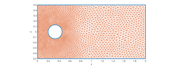
 ν=1/100.\nu=1/100.

Refer to caption
Figure 2. Initial geometry of the domain with the refined mesh.

The volume constant mm is set as the volume of the initial domain Ω0\Omega_{0}, which is refined according to the magnitude of the state solution with the minimum mesh size hmin=1/50hmin=1/50 and a maximum mesh size hmax=1/30hmax=1/30. All the governing equations – the state equation, adjoint equation, state responsible for the deformation fields, and the smooth approximation of the normal vector – are solved using the UMFPACK option. The tolerance, furthermore, is selected to be tol=1×106.tol=1\times 10^{-6}.

4.4.1. Augmented Lagrangian Method

The implementation of aL-algorithm is divided into two parts. Namely, we consider when γ1=1\gamma_{1}=1 and γ2=0\gamma_{2}=0 (which we call as the curlaL-problem), γ1=0\gamma_{1}=0 and γ2=1\gamma_{2}=1 (which we call as the detgradaL-problem).

The values of the constants α\alpha, 0\ell_{0}, b0b_{0}, τ\tau, and b¯\overline{b} are chosen so as to maintain stability of the method.

Implementation of curlaL-problem (γ1=1,γ2=0\gamma_{1}=1,\gamma_{2}=0). For this implementation, we have chosen the numerical parameters shown in Table 1.

Table 1. Parameter values for curlaL-problem
Parameter Value Parameter Value
α\alpha 6.0 0\ell_{0} 20
b0b_{0} 1×1041\times 10^{-4} τ\tau 1.05
b¯\overline{b} 10

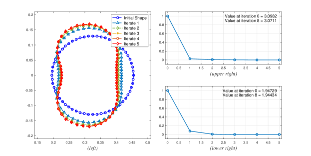
Using these parameters, the evolution of the free-boundary is shown in Figure 3(left) below. We see that the free-boundary evolves into a bean-shaped surface.

Refer to caption
Figure 3. From curlaL-problem, the figure features the following: (left) Evolution of the free-boundary Γf\Gamma_{\rm f}, (upper right) Normalized trend of the objective functional, (lower right) Normalized trend of the volume

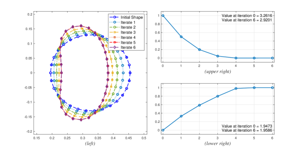
As expected, we see that the value of the objective functional decreases on each iteration (see Figure 3(upper right)). In fact, the value of the objective functional decreases by 10.47%10.47\%. Lastly, we see from Figure 3(lower right) that the volume increases by 0.58%0.58\%.

Implementation of detgradaL-problem (γ1=0,γ2=1\gamma_{1}=0,\gamma_{2}=1). In this particular scenario, we consider the parameter values shown in Table 2.

Table 2. Parameter values for detgradaL-problem
Parameter Value Parameter Value
α\alpha 1.3 0\ell_{0} .5
b0b_{0} 1×10²¹\times 10^{-2} τ\tau 1.05
b¯\overline{b} 10

Unlike the curlaL-problem, the shape does not evolve into a bean-shaped obstacle. The evolution acts in a non-symmetrical manner (see Figure 4(left)) due to the fact that the right hand-side of the adjoint equation with the current choice of γ1\gamma_{1} and γ2\gamma_{2} is also non-symmetric. Even though this problem runs seven iterations, it can be observed that after two iterations, the shapes are almost identical as shown in Figure 4(left). This phenomena can also be observed on the trend of the decrease of the value of the objective functional, i.e., the values of the functional from the second iteration up to the last iteration differ minimally.

Refer to caption
Figure 4. From detgradaL-problem, the figure features the following: (left) Evolution of the free-boundary Γf\Gamma_{\rm f}, (upper right) Normalized trend of the objective functional, (lower right) Normalized trend of the volume

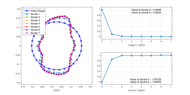
The percentage change from the initial shape to the second iterate-shape is 3.67%3.67\%, while from the second iterate to the final shape it is 0.03%0.03\%. In general, from the initial shape to the final shape the percentage difference is 3.7%.3.7\%. We also point out that the minute difference of iterate 2 and the final shape may be caused by the fact that the changes are caused by mesh adaptation used in our program.

4.4.2. Divergence-free deformation fields

Unlike the implementation of aL-algorithm, the minimization problem is solved by dF-algorithm in three parts. In particular, we shall illustrate the following modificatoins:

  1. \bullet

    curldF-problem with parameters γ1=1\gamma_{1}=1, and γ2=0\gamma_{2}=0;

  2. \bullet

    detgraddF-problem with parameters γ1=0\gamma_{1}=0, and γ2=1\gamma_{2}=1;

  3. \bullet

    mixeddF-problem with parameters γ1,γ21\gamma_{1},\gamma_{2}\geq 1.

Implementation of curldF-problem (γ1=1,γ2=0\gamma_{1}=1,\gamma_{2}=0). Note that in using dF-algorithm, we are more relaxed in the choice of the parameters. In particular, we are just concerned with the parameter α\alpha which we choose as α=5\alpha=5.

As we can see in Figure 5(left) the method converges to a bean shaped boundary, just like the generated shape in curlaL-problem. However, in the current case, the method steers the shape to have the inner domain bounded by Γf\Gamma_{\rm f} lose its convexity on the left side.

Refer to caption
Figure 5. From curldF-problem, the figure features the following: (left) Evolution of the free-boundary Γf\Gamma_{\rm f}, (upper right) Normalized trend of the objective functional, (lower right) Normalized trend of the volume

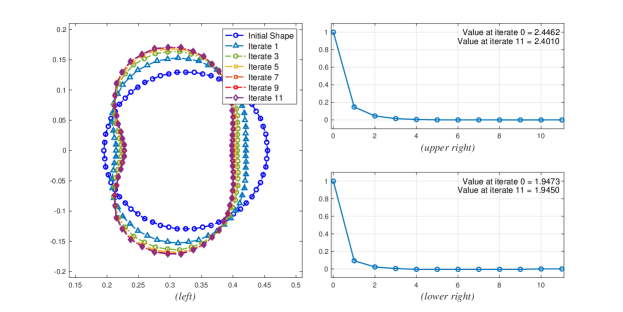
One can also infer from Figure 5(upper right) that the relative difference - with respect to the initial shape - of the value of the objective function at the optimal shape is 1.85%1.85\%, while of the volume is 0.12%0.12\%.

If we compare this algorithm with aL-algorithm with α=5\alpha=5 and 0=13,13.5,14\ell_{0}=13,13.5,14, we deduce from Figure 6(lower right) that our current method preserves the volume better. We also see from Figure 6(upper right)) that the objective function values using dF-algorithm are lower than the ones from aL-algorithm except from the case 0=14\ell_{0}=14, which fails horribly with volume preservation.

Refer to caption
Figure 6. (left) Comparison of final shapes between aL-algorithm and dF-algorithm for the problem with the parameters γ1=1\gamma_{1}=1, γ2=0\gamma_{2}=0 and α=5\alpha=5, (upper right) Comparison of objective value trends between aL-algorithm and dF-algorithm, (lower right) Comparison of volume trends between aL-algorithm and dF-algorithm

We also see in Figure 6(left) what we meant we we said that the inner domain bounded by Γf\Gamma_{\rm f} loses its convexity on the right side, i.e., the curvature of the shapes generated by aL-algorithm are more pronounced compared to our current algorithm.

Remark 6.

(i.) The reason why we started the simulation of aL-algorithm with α=5\alpha=5 at 0=13\ell_{0}=13 is that if we try a smaller value of 0\ell_{0}, the scheme becomes too stringent and will not generate any domain perturbation.

(ii.) One interesting feature in Figure 6 is that even after ten iterations, the objective function and volume trends for the case 0=14\ell_{0}=14 seem to have not converged yet. In fact, even after 20 iterations, the scheme still finds a descent direction. This highlights an issue with the balance between regularization and stability, which is an interesting venture to delve into if one is keen on studying stability of numerical methods. One may also refer to [27] for some insights on the issue of regularity and stability in general.

Implementation of detgraddF-problem (γ1=0,γ2=1\gamma_{1}=0,\gamma_{2}=1). Similar with our previous implementation, we only needed to choose a value for the parameter α\alpha, which in this case is α=1.0.\alpha=1.0.

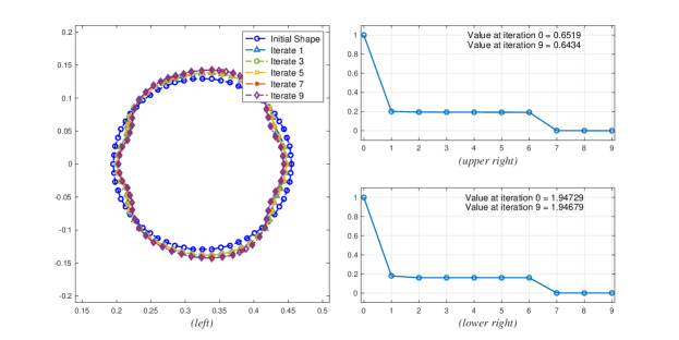
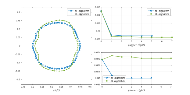
As illustrated in Figure 7(left), the final perturbed domain differs minimally from the initial domain. Furthermore, we can see from Figure 8(left) that the deformation is less extensive as compared to the final shapes generated by the aL-algorithm. One can also infer from Figure 7(upper and lower right) that the value of the objective function and of the volume at the final shape differs relatively (w.r.t. the initial shape) by 1.30%1.30\% and 0.03%0.03\%, respectively. This implies that the volume preservation is significantly satisfied by the dF-algorithm, while maintaining a significant decrease on the objective function.

Refer to caption
Figure 7. From detgraddF-problem, the figure features the following: (left) Evolution of the free-boundary Γf\Gamma_{\rm f}, (upper right) Normalized trend of the objective functional, (lower right) Normalized trend of the volume

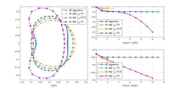
If we compare the current algorithm to aL-algorithm with the same value of α\alpha, we see from Figure 8(lower right) that the only value of 0\ell_{0} that can preserve the initial volume better is 0=0.1\ell_{0}=0.1. We also see from Figure 8(upper right) that since the difference between the final value of the objective function at the final shape using dF-algorithm and aL-algorithm with 0=0.1\ell_{0}=0.1 is very minimal, the aL-algorithm is more preferable. The only drawback though is that aL-algorithm depends on more parameters, hence it is more subject to instabilities.

Refer to caption
Figure 8. (left) Comparison of final shapes between aL-algorithm and dF-algorithm with the parameters γ1=0\gamma_{1}=0, γ2=1\gamma_{2}=1, and α=1\alpha=1, (upper right) Comparison of objective value trends between aL-algorithm and dF-algorithm, (lower right) Comparison of volume trends between aL-algorithm and dF-algorithm

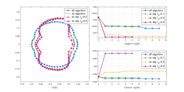
The implementations of the aL-algorithm with 0=0.2,0.4\ell_{0}=0.2,0.4 exhibit a significant decrease on the objective functional as compared to the dF-algorithm, however they both violate the volume constraint significantly.

To illustrate another case where the aL-algorithm is more preferable for the minimization of the detgrad functional, Figure 9 shows an implementation where α=1.2\alpha=1.2, and 0=0.1\ell_{0}=0.1 for the aL-algorithm.

Refer to caption
Figure 9. (left) Comparison of final shapes between aL-algorithm and dF-algorithm with the parameters γ1=0\gamma_{1}=0, γ2=1\gamma_{2}=1, and α=1.2\alpha=1.2, (upper right) Comparison of objective value trends between aL-algorithm and dF-algorithm, (lower right) Comparison of volume trends between aL-algorithm and dF-algorithm

As can be easily observed in Figure 9(right), aL-algorithm yields better result when it comes to the minimization of the objective functional and preservation of the volume. In particular, the objective functional values are much lower for aL-algorithm, and the volume difference between the initial and final shape are much closer compared to the values generated by dF-algorithm.
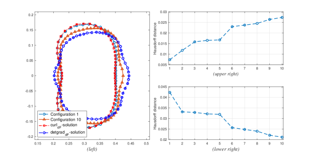
Implementation of mixeddF-problem (γ1,γ21\gamma_{1},\gamma_{2}\geq 1). In this implementation, we consider several configurations for reasons we shall explain later. In particular, we shall consider the value of parameters as shown in Table 3.

Table 3. Parameter Values for mixeddF-problem
Configuration α\alpha γ1\gamma_{1} γ2\gamma_{2}
1 6.0 1.0 1.0
2 7.0 1.0 2.0
3 8.0 1.0 3.0
4 9.0 1.0 4.0
5 10.0 1.0 5.0
6 11.0 1.0 6.0
7 12.0 1.0 7.0
8 13.0 1.0 8.0
9 14.0 1.0 9.0
10 15.0 1.0 10.0

For the first configuration, Figure 10 shows how the initial shape evolves into a bean shaped boundary similar with that of curldF-problem. Furthermore, the value of the objective functional at the final shape differs relatively from the initial shape by 0.87%0.87\% while the volume is preserved with a relative difference of 0.30%0.30\%.

Refer to caption
Figure 10. From configuration 1 of mixeddF-problem, the figure features the following: (left) Evolution of the free-boundary Γf\Gamma_{\rm f}, (upper right) Normalized trend of the objective functional, (lower right) Normalized trend of the volume

We note that in this configuration the final shape is almost the same with the final shape generated by curldF-problem, as shown in Figure 11(left).

Refer to caption
Figure 11. (left) Plots of the solutions of mixeddF-problem (using configuration 1), of curldF-problem and of detgraddF-problem generated boundaries, (upper right) Comparison of the objective function value of the curldf-problem and the curl part of the mixeddF-problem, (lower right) Comparison of the objective function value of the curldF-problem and the detgrad part of the mixeddf-problem

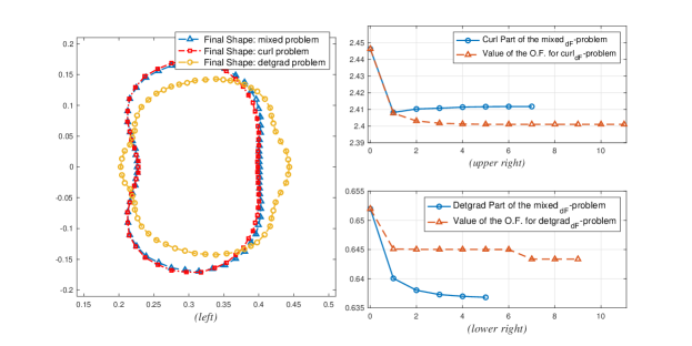
To understand why this phenomena occurs, we note that the objective function in our configurations can be written as

𝒥(Ω)=[5Γfds12Ω|×𝐮|dx]+k[ΓfdsΩh(det(𝐮))dx],\mathcal{J}(\Omega)=\left[5\int_{\Gamma_{\rm f}}\operatorname*{d\!}s-\frac{1}{2}\int_{\Omega}|\nabla\times{\operatorname{\boldsymbol{u}}}|\operatorname*{d\!}x\right]+k\left[\int_{\Gamma_{\rm f}}\operatorname*{d\!}s-\int_{\Omega}h(\mathrm{det}(\nabla{\operatorname{\boldsymbol{u}}}))\operatorname*{d\!}x\right],

where kk is the configuration number. We shall call the first bracket as the curl part of the mixeddf-problem while the other one the detgrad part. Evaluating the two parts numerically at the initial shape, we can see in Figure 11(right) that the value of the curl part is higher than the detgrad part, with the respective values 2.452.45 and 0.650.65. This results to having the optimization problem prioritize minimizing the curl part of the mixeddF-problem, and this results into having the similar shape as that of the curldF-problem. Intriguingly though, when compared to the values of the objective functional for the curldF-problem and the detgraddF-problem, the values of the curl part on each iterate is much higher than the objective function for curldF-problem (see Figure 11(upper right)) while the values of the detgrad part is lower than the objective function for detgraddF-problem (see Figure 11(lower right)).

To investigate the influence of the curldF-problem and the detgraddF-problem to the solution obtained by mixeddF-problem even further, we implement configuration 2. In this example, the value of the detgrad part is higher than the one considered on the previous configuration.

Refer to caption
Figure 12. (left) Plots of the solutions of mixeddF-problem (using configuration 2), of curldF-problem and of detgraddF-problem generated boundaries, (upper right) Comparison of the objective function value of the curldF-problem and the detgrad part of the mixeddF-problem, (lower right) Comparison of the objective function value of the curldF-problem and the detgrad part of the mixeddF-problem

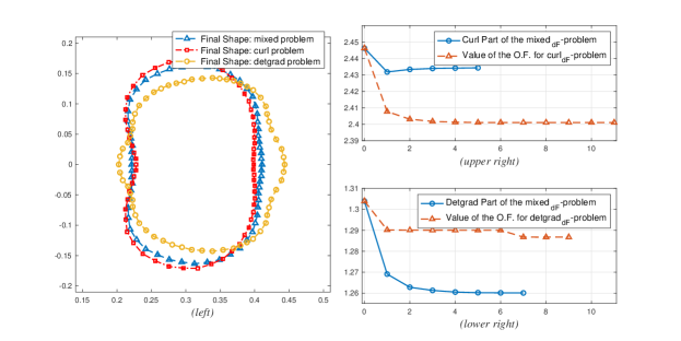
As can be observed on Figure 12(left) the final shape for the mixeddF-problem is now more distinct from that of the curldF-problem. In particular, we now see a bump emerging on the right side of the final shape for mixeddF-problem. The emergence of such bump may be attributed to its presence on the final shape of detgraddF-problem. In fact, the value of the detgrad part is now higher compared to the previous configuration (see Figure 12(upper right) and (lower right)).

Skipping to the fourth configuration, we see that value of the detgrad part is higher than the curl part. From Figure 13(left), the final shape of the mixeddf-problem is now greatly influenced by the shape of detgraddf-problem. In particular, it can be observed that the right side of the shape generated by mixeddf-problem converges to the shape induced by the detgraddf-problem. However, we can still observe the effect of the shape by the curldf-problem on the left side.

Refer to caption
Figure 13. (left) Plots of the solutions of mixeddF-problem (using configuration 4), of curldF-problem and of detgraddF-problem generated boundaries, (upper right) Comparison of the objective function value of the curldF-problem and the detgrad part of the mixeddF-problem, (lower right) Comparison of the objective function value of the curldF-problem and the detgrad part of the mixeddF-problem

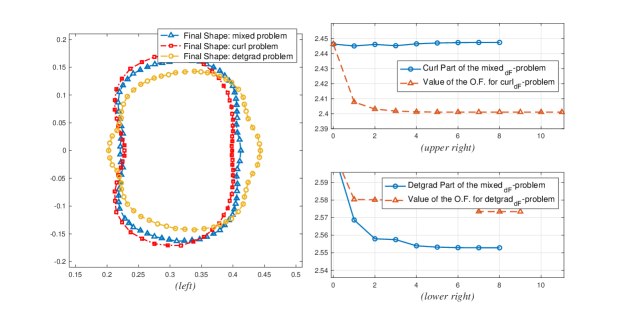
To see the convergence more clearly we utilize Hausdorff distance. Figure 14(upper right) illustrates the increase of the Hausdorff distance between the solutions of the mixeddF-problem and the curldF-problem. Meanwhile, Figure 14(lower right) shows a decreasing trend in the Hausdorff distance between the solutions of the mixeddF-problem and the detgraddF-problem.

Refer to caption
Figure 14. (left) Plots of the solutions of mixeddF-problem (configurations 1 and 10), of curldF-problem, and of detgraddF-problem, (upper right) Hausdorff distance between mixeddF-solution and curldF-solution on each configuration, (lower right) Hausdorff distance between mixeddF-solution and detgraddF-solution on each configuration

4.5. Effects of the Shape Solutions to Generation of Twin-Vortex

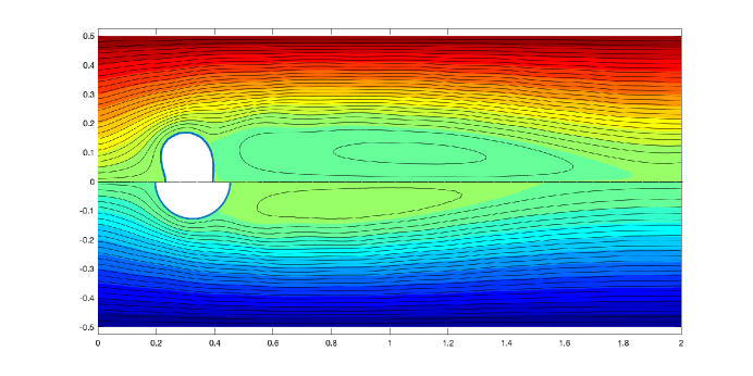
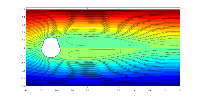
We conclude this section by briefly illustrating the effects of the final shapes to twin-vortices induced by a time-dependent Navier–Stokes equations right before the shedding of Karman vortex, and is solved using a stabilized Lagrange–Galerkin method [29]. Since similar behaviors can be observed if we use aL-algorithm or dF-algorithm, we only illustrate the cases using dF-algorithm.

Figure 15 shows the comparison of the twin-vortices using the initial domain and the domain obtained from curldF-problem. The figure shows that the solution to the curldF-problem generates a longer vortex compared to that of the initial domain.

Refer to caption
Figure 15. The figure shows the comparison of the flows using the initial domain (lower part), and the final shape from curldf-problem (upper part)

Similarly, the solution of the detgraddF-problem generates a longer vortex as compared to the initial domain as shown in Figure 15.

Refer to caption
Figure 16. The figure shows the comparison of the flows using the initial domain (lower part), and the final shape from detgraddf-problem (upper part)

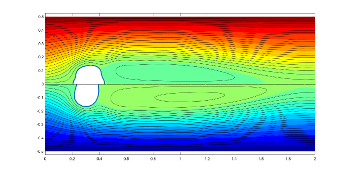
Lastly, Figure 17 shows that the vortex generated using the final shape of curldf-problem is longer than that of the detgraddf-problem.

Refer to caption
Figure 17. The figure shows the comparison of the flows using the the final shape from curldf-problem (lower part), and the final shape from detgraddf-problem (upper part)
Remark 7.

As mentioned before, the generation of vortices gives a possible application of our shape optimization problem to a branch of machine learning known as physical reservoir computing. According to Goto, K., et.al.[13], the length or the long diameter of the twin-vortices has a correlation with the memory capacity - as defined in the aforementioned reference - of the physical reservoir computer. With our previous observations, we can naively conjecture that the shapes generated by the implementations above will cause a better memory capacity for the physical reservoir computer. However, since these are just visual observations, we need more experiments to verify that these shapes indeed generate a good computational ability.

5. Conclusion

We presented a minimization problem that is intended to maximize the vorticity of the fluid governed by the Stokes equations. Furthermore, we considered a Tikhonov-type regularization - in the form of the perimeter functional - and a volume constraint. The shape sensitivity analysis is carried out by utilizing the rearrangement method which gave us the necessary conditions in the form of the Zolesio–Hadamard Structure. We then implemented the necessary conditions in two ways, one is by utilizing the augmented Lagrangian, and by utilizing a new method for solving the deformation field that possesses the divergence-free condition. From these methods, we showed some numerical examples. Lastly, we illustrated how the shape solutions affect the flow, and we briefly mentioned a possible application of this problem in the field of physical reservoir computers.

We end this note by pointing out that the investigation in the stability of the numerical approaches with respect to the parameters were only scratched on the surface and can be explored with more rigor. Furthermore, the visual observations on the emergence of the twin-vortex are not enough to give a good conclusion with regards to the memory capacity of the physical reservoir computer. With this, one can investigate even further and try some more tests as carried out in [13].

References

  • [1] H. Azegami. Solution of shape optimization problem and its application to product design. In Hiromichi Itou, Masato Kimura, Vladimír Chalupecký, Kohji Ohtsuka, Daisuke Tagami, and Akira Takada, editors, Mathematical Analysis of Continuum Mechanics and Industrial Applications, pages 83–98, Singapore, 2017. Springer Singapore.
  • [2] J. Bacani and G. Peichl. On the first-order shape derivative of the Kohn–Vogelius cost functional of the Bernoulli problem. Abstract and Applied Analysis, 2013:1–19, 2013.
  • [3] D. Chenais. On the existence of a solution in a domain identification problem. Journal of Mathematical Analysis and Applications, 52(2):189 – 219, 1975.
  • [4] M. S. Chong, A. E. Perry, and B. J. Cantwell. A general classification of three‐dimensional flow fields. Physics of Fluids A: Fluid Dynamics, 2(5):765–777, 1990.
  • [5] C. Dapogny, P. Frey, F. Omnès, and Y. Privat. Geometrical shape optimization in fluid mechanics using freefem++. Structural and Multidisciplinary Optimization, 58(6):2761–2788, 2018.
  • [6] M. Delfour and J.-P. Zolesio. Shapes and Geometries: Metrics, Analysis, Differential Calculus, and Optimization. Society for Industrial and Applied Mathematics, 3600 Market Street, 6th Floor, Philadelphia, PA 19104-2688 USA, 2 edition, 2011.
  • [7] M. Desai and K. Ito. Optimal controls of Navier–Stokes equations. SIAM Journal on Control and Optimization, 32(5):1428–1446, 1994.
  • [8] M. F. Eggl and Peter J. Schmid. Mixing enhancement in binary fluids using optimised stirring strategies. Journal of Fluid Mechanics, 899:A24, 2020.
  • [9] L.C. Evans. Partial Differential Equations. Graduate studies in mathematics. American Mathematical Society, 1998.
  • [10] T. L. B. Flinois and T. Colonius. Optimal control of circular cylinder wakes using long control horizons. Physics of Fluids, 27(8):087105, 2015.
  • [11] Z. M. Gao, Y. C. Ma, and H. W. Zhuang. Shape optimization for navier–stokes flow. Inverse Problems in Science and Engineering, 16(5):583–616, 2008.
  • [12] V. Girault and P.-A. Raviart. Finite Element Methods for Navier-Stokes Equations: Theory and Algorithms, volume 5 of Springer Series in Computational Mathematics. Springer, Berlin, Heidelberg, 1986.
  • [13] K. Goto, K. Nakajima, and H. Notsu. Twin vortex computer in fluid flow. New Journal of Physics, 23(6):063051, jun 2021.
  • [14] J. Haslinger, K. Ito, T. Kozubek, K. Kunisch, and G. Peichl. On the shape derivative for problems of Bernoulli type. Interfaces and Free Boundaries, 11(2):231–251, 2006.
  • [15] J. Haslinger, J. Málek, and J. Stebel. Shape optimization in problems governed by generalised navier-stokes equations: Existence analysis. Control and cybernetics, 34:283–303, 03 2005.
  • [16] F. Hecht. New development in freefem++. J. Numer. Math., 20(3-4):251–265, 2012.
  • [17] A. Henrot and M. Pierre. Shape Variation and Optimization: A Geometrical Analysis. EMS Tracts in Mathematics, 28 edition, 2014.
  • [18] A. Henrot and Y. Privat. What is the optimal shape of a pipe? Archive for Rational Mechanics and Analysis, 196(1):281–302, 2010.
  • [19] J. C. R. Hunt, A. A. Wray, and P. Moin. Eddies, streams, and convergence zones in turbulent flows. In Proc. 1988 Summer Program of Center for Turbulence Research Program, 1998.
  • [20] Ito, K., Kunisch, K., and Peichl, G. H. Variational approach to shape derivatives. ESAIM: COCV, 14(3):517–539, 2008.
  • [21] Y. Iwata, H. Azegami, T. Aoyama, and E. Katamine. Numerical solution to shape optimization problems for non-stationary navier-stokes problems. JSIAM Letters, 2:37–40, 2010.
  • [22] Jinhee Jeong and Fazle Hussain. On the identification of a vortex. Journal of Fluid Mechanics, 285:69–94, 1995.
  • [23] H. Kasumba and K. Kunisch. Vortex control in channel flows using translational invariant cost functionals. Computational Optimization and Applications, 52(3):691–717, 2012.
  • [24] G. Mather, I. Mezić, S. Grivopoulos, U. Vaidya, and L. Petzold. Optimal control of mixing in Stokes fluid flows. Journal of Fluid Mechanics, 580:261–281, 2007.
  • [25] B. Mohammadi and O. Pironneau. Applied Shape Optimization for Fluids. NUMERICAL MATHEMATICS AND SCIENTIFIC COMPUTATION. Oxford University Press, 2010.
  • [26] P. Monk. Finite Element Methods for Maxwell’s Equations. Oxford University Press, 2003.
  • [27] M. T. Nair, M. Hegland, and R. S. Anderssen. The trade-off between regularity and stability in tikhonov regularization. Mathematics of Computation, 66(217):193–206, 1997.
  • [28] J. Nocedal and S. Wright. Numerical Optimization, volume 2 of Springer Series in Operations Research and Financial Engineering. Springer-Verlag New York, 2006.
  • [29] Notsu, H. and Tabata, M. Error estimates of a stabilized lagrange-galerkin scheme for the navier-stokes equations. ESAIM: M2AN, 50(2):361–380, 2016.
  • [30] M. Pošta and T. Roubíček. Optimal control of Navier–Stokes equations by Oseen approximation. Computers & Mathematics with Applications, 53(3):569–581, 2007. Recent Advances in the Mathematical Analysis of Non-Linear Phenomena.
  • [31] J. F. T. Rabago and H. Azegami. An improved shape optimization formulation of the bernoulli problem by tracking the neumann data. Journal of Engineering Mathematics, 117(1):1–29, 2019.
  • [32] J. F. T. Rabago and H. Azegami. A second-order shape optimization algorithm for solving the exterior Bernoulli free boundary problem using a new boundary cost functional. Computational Optimization and Applications, 2020.
  • [33] S. Schmidt and V. Schulz. Shape derivatives for general objective functions and the incompressible navier-stokes equations. Control and Cybernetics, 39(3):677–713, 2010.
  • [34] J. Sokolowski and J.-P. Zolesio. Introduction to Shape Optimization: Shape Sensitivity Analysis. Springer Series in Computational Mathematics. Springer-Verlag Berlin Heidelberg, 1 edition, 1992.