A shared-revenue Bertrand game
Abstract.
We introduce and analyze a variation of the Bertrand game in which the revenue is shared between two players. This game models situations in which one economic agent can provide goods/services to consumers either directly or through an independent seller/contractor in return for a share of the revenue. We analyze the equilibria of this game, and show how they can predict different business outcomes as a function of the players’ costs and the transferred revenue shares. Importantly, we identify game parameters for which independent sellers can simultaneously increase the original player’s payoff while increasing consumer surplus. We then extend the shared-revenue Bertrand game by considering the shared revenue proportion as an action and giving the independent seller an outside option to sell elsewhere. This work constitutes a first step towards a general theory for how partnership and sharing of resources between economic agents can lead to more efficient markets and improve the outcomes of both agents as well as consumers.
1. Introduction
1.1. Motivation
Many modern businesses partner with independent service providers to increase efficiency. One method through which this is done is for a company to let a separate company provide services/goods to customers in exchange for a share of the revenue. The independent service provider in turn may benefit from the wider visibility it gains through access to the original company’s pool of customers. This is seen in a number of real-world scenarios, including but not limited to:
-
(A)
Consider a large store which allows independent sellers to use some of its shelf space to sell products in return for a portion of the selling price. The large store may of course obtain the same products from a vendor and sell them on its own, and the independent seller may set up its own store, but depending on the costs for each party, both parties might benefit from having the independent seller’s products available in the larger store.
-
(B)
Consider a construction and maintenance company, with a large pool of customers, providing a variety of services such as plumbing, repairs, painting services, etc. The company can either provide a specific service on its own, or refer the customer to a contractor who sets the price for the service, and pays the original company a referral fee.
-
(C)
Consider a ridesharing or taxi platform. When a passenger requests a ride, they have the option of transporting the passenger with either (i) a self-driving car, owned by the ridesharing platform, or (ii) an independent human driver, whom the ridesharing platform charges a fee for each passenger they refer.
-
(D)
A large airline could either operate a short regional flight with their own aircraft or allow a regional partner to operate the flight.
-
(E)
A healthcare provider can either provide specialist services in-house or refer their patients to an external contractor, charging a referral fee.
1.2. Overview
In this work we provide a game theoretic model for reasoning about the interaction between agents in scenarios such as these with a variation of the Bertrand pricing game (Bertrand, 1883). For concreteness, we will focus our intuition and analysis on scenario (A) from Section 1.1, though our model can explain phenomena in domains far beyond retail sales. In accordance with scenario (A), the “shared-revenue Bertrand game” is played between a retailer, and an independent goods/services provider which we will refer to as the independent seller (seller). Both players sell an identical good/service, with each agent having a different cost. Under the revenue sharing program, whenever the independent seller fulfills demand, a portion of the revenue, called the referral fee, is transferred from the independent seller to the retailer. In Section 2, we set up the game in more detail, then in Section 3 we identify the Nash equilibria of this game. In Section 4, we interpret and analyze the equilibria of the shared-revenue Bertrand game in depth with different costs and fee structures.
The referral fee is a constant parameter of the shared-revenue Bertrand game of Section 2. However, to make the game more realistic, in Section 5 we introduce the “fee optimization game,” which models the referral fee as an action for the retailer that is chosen before playing the shared-revenue Bertrand game. Finally, in Section 6, we introduce the “outside option game”: after observing the referral fee chosen by the retailer, the independent seller can choose to sell on their own instead of through the retailer.
The equilibria of the “fee optimization game” reveal that the retailer always prefers to allow the independent seller to fulfill demand in equilibrium, setting the referral fee strategically so as to maximize their payoff. There is a sweet spot for the optimal fee such that it is low enough to stimulate economic activity while high enough to maximize payoff. In the fee optimization game of Section 5, we still observe some unrealistic equilibria in which the retailer sets such a high fee that the independent seller must fulfill demand at their effective cost (thus achieving no payoff), which leads us to consider the “outside option game” in Section 6. If the independent seller’s threat of selling on their own is credible, the unrealistic equilibria of Section 5 will no longer be observed, as the retailer must set the referral fee lower to ensure the independent seller doesn’t exercise their outside option. Importantly, our analysis demonstrates that the retailer will frequently be incentivized to set a fee under which both the independent seller increases its payoff compared to selling independently, and the price to the customer is decreased relative to the price either the retailer or the independent seller would have set independently. Our results therefore suggest that such a revenue sharing mechanism can not only increase social welfare, but also simultaneously improve outcomes for both players as well as consumers.
In each of the models, we examine if the revenue sharing program increases the retailer’s payoff compared to simply fulfilling demand on their own, and how it affects the end cost to the customer.
1.3. Related work
Our model is an extension of the standard Bertrand game (Bertrand, 1883) in which two sellers of an identical product with the same cost set their prices independently. As we justify in Appendix B, we consider the regime in which the sellers’ costs are asymmetric, which is a natural extension of the standard Bertrand game, studied for instance in (Blume, 2003; Kartik, 2011; Demuynck, 2019).
One field in which revenue sharing programs as described in Section 1.1 have been studied is in the independent contractor literature. Much of this literature analyzes relationships with independent contractors through the framework of principal agent theory (Coats, 2002; Chang, 2014). The revenue-sharing program can also be seen as a form of “make-or-buy” decision for the retailer (Coase, 1937; Williamson, 1975; Tadelis, 2002). Slightly less obviously, another field in which revenue sharing programs have been studied is optimal taxation theory, where the referral fee can be viewed as the retailer imposing a tax on the independent seller. Viewed in this light, our results about optimal referral fees resonate strongly with optimal taxation theories such as (Laffer, 2004; Stern, 1976; Stiglitz, 1987).
Finally, the idea of an outside option that we introduce in Section 6 is common in negotiation and bargaining theory (Binmore et al., 1989; Osborne and Rubinstein, 1990), which makes sense because the participation of the independent seller in the retailer’s revenue-sharing program can be seen as a negotiation of a contract. In fact, there is even an “outside option principle” (Watson, 2020), which informally states than an outside option must be credible in order to have an effect on the Nash equilibria of the game; our results are consistent with this.
2. Preliminaries
Our model is a game in which two players – the retailer (), and the independent seller (), sell an identical product. The actions in the game are the price each player chooses to charge, and we assume the players move simultaneously. Formally, we define the following game:
Shared-Revenue Bertrand Game
Parameters
Retailer’s cost , seller’s cost , referral fee
Gameplay
-
(1)
The retailer and seller simultaneously choose prices, yielding a price configuration
The payoffs for the players are
| (1) | ||||
| (2) |
where , , and denote prices, costs, quantities sold and the referral fee, respectively, and subscripts denote the players. This game can be viewed as a modification of the Bertrand game, where the players have different costs, and a portion of the independent seller’s revenue is shared with the retailer as part of the service provided by the retailer.
To allow for a concrete mathematical analysis we assume demand is linear in price, and that the agent with the lower price fulfills all demand. When both players set the same price, we assume they split the market where the retailer fulfills of the demand and the independent seller fulfills the rest. This assumption is made for mathematical completeness, although in Proposition 1 we show that no split market equilibrium exists, making the choice of irrelevant. Concretely, the retailer’s demand curve is given by
| (3) |
where and are constant parameters. The demand curve for the independent seller is analogous, but is replaced by .
To reduce the number of parameters in the model we will use the following normalization, and throughout the rest of the paper present the results in terms of unitless variables
| (4) |
Under this normalization, the demand at price is 1, and the demand at price is . Equations (1) and (2) remain unchanged if we remove bars, and (3) reduces to
| (5) |
2.1. Necessary assumptions
In order for the game to be nontrivial, we must impose the following constraints:
-
(I)
There exists a price at which both the retailer and independent seller could achieve a nonzero payoff when fulfilling demand ().
-
(II)
The seller’s cost is less than the retailer’s cost ().
-
(III)
The referral fee takes some, but not all of the independent seller’s revenue ().
In Appendix B, we formally show that the game degenerates if these are violated, but the importance of each condition should be fairly intuitive. Overall, the revenue-sharing program should be thought of as for products that the retailer could conceivably sell themselves, but the independent seller is able to do so more efficiently.
2.2. Important prices and payoffs
We now introduce several important prices and corresponding payoffs which will be used throughout this paper. We also include a full notation table in Appendix A, and include derivations of the key prices and fees in Appendix D.
As we will later prove in Proposition 1, we only need to focus on cases where either the retailer or the independent seller fulfill all demand, and can ignore any split market scenario. When we write a payoff with two subscripts, the first denotes the the player whose payoff we refer to, and the second denotes the player who fulfills all demand. Thus, and are the retailer’s and the independent seller’s payoffs when the retailer fulfills all the demand, respectively. Similarly and are the retailer’s and the independent seller’s payoffs when the independent seller fulfills all the demand, respectively. Explicitly, it follows from (1), (2), and (5) that
| (6) | ||||
| (7) |
In Figure 1 we plot the payoffs of the players as a function of price for two choices of game parameters . Solid and dashed lines denote the players’ payoff when the retailer or independent seller fulfill all demand, respectively, while blue and red lines denote the payoffs to the retailer and the independent seller, respectively.
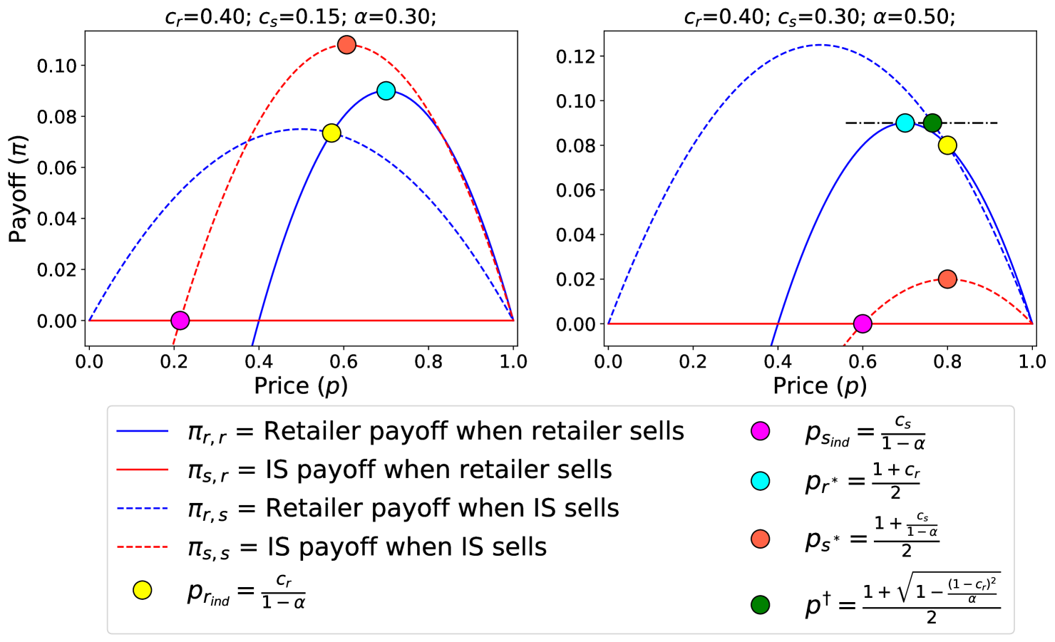
Figure 1 also illustrates five important price points and their corresponding payoffs which will be used throughout this paper. We denote by and the prices each player would set to maximize their own payoff if they fulfilled all demand, and call these the retailer’s or independent seller’s optimal selling price. Differentiating the players’ single agent payoffs and and equating to zero in (36) and (40) gives the values of these prices and their corresponding payoffs –
| (8) | ||||
| (9) |
We denote by and the prices at which the retailer and the independent seller are indifferent to which player fulfills demand, i.e. and . Solving these equations in (38) and (42) yields the following prices and payoffs –
| (10) | ||||
| (11) |
We first note that , and therefore the independent seller’s indifference price is also its breakeven price.
More interestingly, while the retailer’s breakeven price is still its cost, , its indifference price is scaled by , but at that price its payoff is nonzero. This is the main feature which differentiates the shared-revenue Bertrand game from the classical Bertrand game, as the retailer can choose to fulfill demand on its own or allow the independent seller to fulfill demand, making revenue from the fee. As a result, this game gives rise to a more complex equilibrium structure which depends on the fees and costs of the players. Note also that because we assume (Section 2.1), we have .
Next, we introduce the price at which the retailer’s payoff when the independent seller fulfills demand is equal to its optimal payoff had it fulfilled demand on its own, i.e.
| (12) |
is the solution of a quadratic equation which we derive in (58), and we define it as the larger of the two possible solutions. Furthermore, is only well-defined when , and therefore we only show it in the right subplot of Figure 1.
3. Equilibrium analysis
3.1. Market split
For simplicity, we will only consider pure strategies in this paper; thus, a strategy profile can be characterized fully by a tuple denoting the prices chosen by the retailer and independent seller. We first prove, in Proposition 1, that in all equilibria, one player takes the entire market.
Proposition 0.
Let be an equilibrium price configuration, with the equilibrium quantities sold by each player and . Then .
Proof sketch.
To prove the Proposition we show that when the market is split, the retailer’s payoff is a weighted average of and , and one of them is larger than the split market payoff. Thus, the retailer can always increase their payoff by either lowering or raising the price by an infinitesimal amount, fulfilling demand themselves or allowing the independent seller to do so respectively. See Appendix C for the complete proof. ∎
While this result is not surprising given that in nearly all standard non-symmetric game theory models, in equilibrium only one player fulfills all demand, this result is clearly not expected to hold in the real world. Game theory results may mimic the world more closely and arrive at more realistic equilibria in which players split demand by modeling factors such as incomplete information and brand loyalty, but these are beyond the scope of this work.
3.2. Nash equilibrium derivation
In light of Proposition 1, we can denote all equilibria in the game by either unequal prices or a shared price , where denotes the player who fulfills the demand. In this subsection, we aim to provide an intuitive sketch of the Nash equilibria.
To narrow our focus, let’s consider shared-price equilibria where the independent seller fulfills demand at price for now. In order for to be an Nash equilibrium, the following conditions must be satisfied:
-
(1)
0 =
-
(2)
-
(3)
If condition 1 doesn’t hold, the independent seller can achieve a higher payoff by increasing its price and letting the retailer fulfill demand. If condition 2 doesn’t hold, the independent seller can increase its payoff by lowering their price and continuing to fulfill all demand. If condition 3 doesn’t hold, then there is some price lower than the retailer can set to take the entire market and increase its payoff.
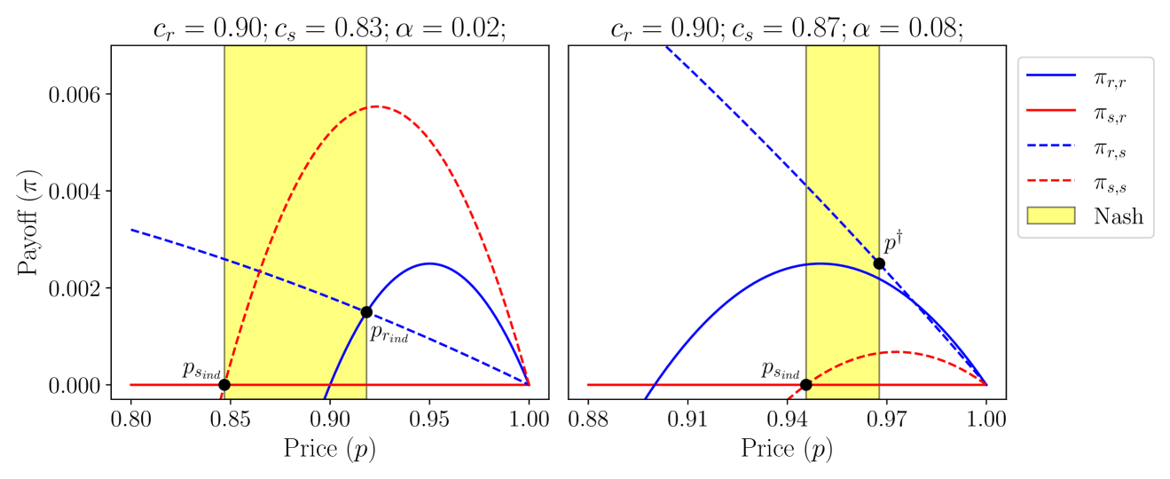
In Figure 2, we highlight in yellow the Nash equilibrium prices where the independent seller fulfills demand. In the left subplot of Figure 2, the Nash equilibria occur at prices , which satisfies all of the Nash equilibrium conditions:
-
(1)
The seller achieves nonnegative payoff because .
-
(2)
The independent seller’s payoff would decrease if they set a price because .
-
(3)
The retailer would not prefer to fulfill demand themselves because .
In the right subplot of Figure 2, the Nash equilibria occur at prices . Just as in the left subplot, conditions 1 and 2 are satisfied because and . Condition 3 is satisfied because . Notice that for the payoff curves in the right subplot, this is a stronger condition than . This stronger condition is necessary because if , the retailer would prefer to set price and achieve a payoff of
In Appendix D.2, we carry forth this intuition and translate conditions 1-3 into feasible intervals of prices for any rather than just for the specific referral fees in Figure 2. For to be a Nash equilibrium, we find that the price must satisfy
| (13) |
We acknowledge that it’s still not clear what the equilibrium interval of prices look like for each possible choice of , namely what lower and upper bounds are attained for each possible referral fee – this warrants a longer discussion which we defer to Section 3.3. For instance, is not well-defined for small , but we will soon see in (20) that whenever is nonempty, is high enough for to be well-defined. For now, simply keep in mind that (13) is sufficient only for shared-price Nash equilibria where the independent seller fulfills demand.
In Appendix D.1, we derive the conditions analogous to (13) for shared-price equilibria where the retailer fulfills demand and find the following:
| (14) |
Upon further inspection of (14), we notice a subtle problem. Recall that always because . Thus, the interval is empty for all , which implies there are no shared price-equilibria where the retailer fulfills demand!
This completes the first step of our analysis for shared-price equilibria, but we also need to consider unequal-price equilibria. Indeed, we consider equilibria where in Appendix D.3 and equilibria where in Appendix D.4. Interested readers can find conditions similar to (13) and (14) in the corresponding appendices; we also include a summary of all Nash equilibria with both equal and unequal prices in Section 3.4.
3.3. Important fees for transitions between Nash equilibria
In this section, we answer the aforementioned question of what the interval in (13) looks like for different values of . To do this, we will introduce five threshold fees that delineate the transitions between when different Nash equilibria can occur (skip ahead to Figure 3 for a preview). Similar analysis as in this section for unequal price equilibria can be found in Appendices D.3 and D.4.
Consider first the left interval of (13), . We know that always. We have so long as , which occurs when . The condition for is not quite as clear, so we introduce the retailer optimal price feasibility fee (derived in (46)) –
| (15) |
The name comes from the fact that is necessary for any equilibrium where the retailer fulfills demand at their optimal price, which we prove in Appendix D.3. Note also that , which we show in (52). Thus, the left interval of (13) is nonempty if and only if .
Now, we turn our attention to the value of , the upper bound of the left interval of (13). This motivates the optimality switching fee (derived in (52)), the seller optimal price feasibility fee (derived in (50)), and the retailer relevance fee (derived in (49)) –
| (16) | ||||
| (17) | ||||
| (18) |
Analogously to , we will soon find that is necessary for an equilibrium where the independent seller fulfills demand at . Intersecting the inequalities in (15), (16), (17), and (18) is sufficient to determine what the left interval of (13) looks like in each region of parameter space. We will omit the algebra here and instead opt to summarize this in Section 3.4. However, throughout the course of the derivation in Appendix D, an important condition emerges that determines the relative ordering of , , and . We show in (54) and (55) that this seller optimal feasibility cost satisfies the following –
| (19) |
Finally, let’s turn our attention to the right interval of (13), . Fortunately, we have already determined the relative ordering of each of the prices in the right interval, except for . For these conditions involving , we introduce the relevance fees for the retailer and seller (derived in (59) and (62)):
| (20) | ||||
| (21) |
Note that we already introduced in (18). The notation arises because we will show that is necessary for any equilibrium where demand is fulfilled at . We don’t include a closed form here for because it is uninsightful, but we remark that and that a closed form is in (62). Finally, the relative ordering of and is complex, and there unfortunately is no special for which . Thus, we will leave that condition unsimplified for now.
3.4. Summary of Nash equilibria
Considering all possible values of and all possible price configurations, we summarize the Nash equilibria of the game below. We denote sets of equilibrium price configurations as and singletons without the set notation, specifically . Recall there are no shared-price equilibria where the retailer fulfills demand, thus all sets of shared-price equilibria implicitly assume that the independent seller is fulfilling demand at price , not the retailer.
Equilibrium Price Configurations of Shared-Revenue Bertrand Game
Notation
We denote Nash equilibrium strategies by price configurations .
Case (i), :
| (22) |
Case (ii), :
| (23) |
4. Refining and interpreting equilibria
In (22) and (23) of the last section, we found a proliferation of Nash equilibrium price configurations in that could be observed given the costs and the value of . However, to help us interpret the Nash equilibria, we would like to discern which price configurations are the “most likely” to occur.
To this end, we introduce some criteria to distinguish Nash equilibria:
-
(1)
Admissibility - A Nash equilibrium in which any player plays a weakly dominated strategy222Player ’s strategy is weakly dominated by strategy if (a) for all strategies of other players , , and (b) there exists a strategy of the other players such that (Rasmusen, 1989). is inadmissible (Govindan and Wilson, 2016).
-
(2)
Relative Pareto optimality - We prefer Nash equilibria that are Pareto optimal333Nash equilibrium is Pareto suboptimal relative to Nash equilibrium if (a) all players weakly prefer, and (b) at least one player strictly prefers over (where “prefer” means achieving a higher payoff) (Rasmusen, 1989). relative to all other Nash equilibria.444Note that a relatively Pareto optimal Nash equilibrium is not necessarily on the Pareto frontier of the game, because it need not be Pareto optimal in the set of all strategies, only in the set of Nash equilibria.
After these two refinements, we will still be left with some intervals of equilibrium prices. However, most of these are inconsequential; in Section 4.3 we will see that these refinements allow us to identify who will fulfill demand and the price at which they will sell in equilibrium.
4.1. Admissibility
The admissibility criterion allows us to rule out any weakly dominated strategies for the retailer and independent seller. For instance, in the left subplot of Figure 2, all Nash equilibrium prices are weakly dominated by for the retailer. Indeed, for all , we have by construction of . Thus, if the seller sets a price , then
| (24) |
which implies that the retailer would have preferred to set price rather than . Thus, the only admissible Nash equilibrium in the left subplot of Figure 2 is .
In Appendix E.1, we more thoroughly consider the retailer and independent seller’s strategies, and find the strategies that are not weakly dominated are
| (25) |
The intuition for the independent seller and the retailer is the same – we can eliminate all prices that are not between their indifference and optimal prices – however, for the retailer we do not always have that . Given the admissible strategies in (25), we can simply intersect the sets of admissible prices with the Nash equilibrium price configurations we found in (22) and (23). For instance, in the right subplot of Figure 2, we find that the admissible Nash equilibria are
We perform these intersections throughout all of parameter space in Appendix E.1, and include a complete summary of admissible equilibria in (70), (71), and (72).
4.2. Relative Pareto optimality
The relative Pareto optimality criterion allows us to further eliminate one admissible equilibrium, which occurs in the following case:
The equilibrium where the retailer fulfills demand at is Pareto suboptimal relative to the shared-price equilibrium where the independent seller fulfills demand. Indeed, by construction of , in both cases the retailer achieves the same payoff of so they are indifferent. However, because implies that , the independent seller achieves a positive payoff when fulfilling demand at while they achieve a payoff of when allowing the retailer to fulfill demand at . Thus, they strictly prefer fulfilling demand at rather than allowing the retailer to fulfill demand at .
As a remark, we note that a reasonable argument could be made for preferring the equilibrium where the retailer fulfills demand at . In this case , so despite the Pareto optimality argument, the customer will be able to buy the product at a lower price if the retailer fulfills demand at instead of the independent seller fulfilling demand at . With this lowest price criterion, would in fact be the most likely equilibrium in this case, as as well. However, whatever we choose does not substantially affect the results, and the relative Pareto optimality criteria will continue to be sensible for us as we generalize the game, thus we proceed with this assumption.
4.3. Equilibrium outcomes
Even after applying these two refinements, inspecting (70), (71), and (72) we can still see that we are left with many intervals of prices. However, in order to interpret the real-world implications of the equilibria, it is prudent to consider the equilibrium outcomes: at what price the customer will purchase the product and from whom they will buy. Indeed, letting the prices be and the fulfiller of demand be , we find the following equilibria:
Equilibrium Outcomes of Shared-Revenue Bertrand Game
Notation
We denote an equilibrium outcome by , indicating that there is an admissible, Pareto optimal Nash equilibrium where player fulfills demand at any price .
Case (i), :
| (26) |
Case (ii), :
| (27) |
Viewing the equilibria in the light of (26) and (27) is incredibly helpful for intepretation; the remainder of Section 4 is dedicated to analyzing the outcomes rather than the price configurations.
A quick glance at (26) and (27) shows that when is sufficiently high, the independent seller is “priced out” of the market and the retailer will fulfill demand at their single agent price as if the independent seller did not exist. When is small, the independent seller sells at the retailer’s indifference price, illustrating that they have to prioritize preventing the retailer from undercutting them over maximizing their own payoff. However, when is in a certain sweet spot, the independent seller may be able to sell at their optimal price in equilibrium. We will see soon that everybody wins in this regime – if the retailer gets to choose the referral fee, they would prefer to choose a referral fee in this sweet spot rather than one that is too high or too low.
4.4. Fee and cost structure analysis
Our results in (26) and (27) show that given a point in the parameter space , we can predict which player will fulfill demand and the price(s) at which they will fulfill demand in an admissible, Pareto optimal Nash equilibrium. In this section, we build intuition about how the parameter space is divided into regions based on these possible equilibria and discuss the business implications for the retailer, both in terms of the retailer’s payoff and in terms of the effect on the prices. Importantly, we will contrast these metrics with the alternative of not having the revenue sharing option available to outside sellers – i.e. compare them with the price the retailer would have set and its payoff in the absence of an independent seller.
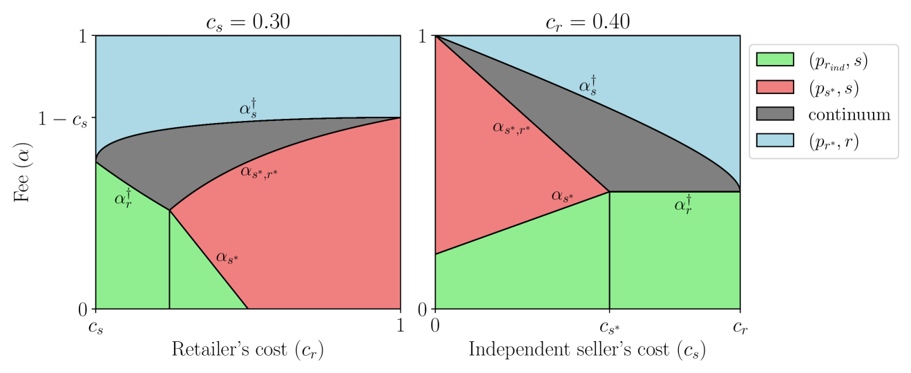
In Figure 3 we plot two cross sections of the parameter space, one plotting vs at a fixed and one with vs at a fixed . The different colors correspond to the admissible, Pareto optimal equilibrium for each set of parameters, with the “continuum” corresponding to the interval of prices .
Notice that when there is no value of that yields an equilibrium in the red region – this is where the notation comes from. Additionally, notice that we may have that , in which case the green region is not feasible as we cannot have .
4.4.1. - The retailer fulfills demand at its single agent price
When (blue region), the fee is too high for the independent seller to fulfill demand, and the game reduces to the retailer “playing” alone and charging its single agent price. This is the least interesting equilibrium if we wish to consider the retailer’s interaction with the independent sellers, but is interesting to be contrasted with all other equilibria as it is the only equilibrium at which the retailer fulfills demand.
4.4.2. A continuum of equilibria in which the independent seller fulfills demand at a price higher than the retailer’s single agent price
When , there are a continuum of equilibrium prices at which the independent seller could fulfill demand (gray region). Note that the independent seller’s price is at least in this region of parameter space, thus the price to the end customer increases relative to a world in which the revenue sharing program did not exist. However, in this region, the retailer achieves at least as much payoff as they would achieve fulfilling demand on their own without the revenue sharing program. Intuitively, this equilibrium is “safe” for the retailer because they will never make less than their single agent payoff, but it comes at the expense of potentially charging customers a higher price.
4.4.3. - The independent seller fulfills demand at the retailer’s indifference price,
When , the independent seller fulfills demand at (green region). In this region there is a trade-off between our two metrics – the retailer’s payoff is lower, but the price for the customer is also lower compared to the retailer selling in a single agent game. Furthermore, the existence of this equilibrium implies that the retailer’s option of selling directly to customer protects the customer from the independent seller charging too high a price when the fee is low.
4.4.4. - The independent seller fulfills demand at their single agent price,
When , we have an equilibrium in which the independent seller fulfills demand at its optimal price (red region). In this regime, we always have , thus the customers are able to purchase at a lower price than they would be able to without the revenue sharing program. Of course, the independent seller prefers this equilibrium because the fee is fairly low and they are able to sell at their optimal price. Finally, it’s even possible that there exists some in the red region such that the retailer achieves a payoff higher than their optimal single agent payoff, yielding a win-win-win situation for the customers, independent seller, and retailer.
5. Optimizing the referral fee
In Section 4.4, we identified an equilibrium that is a win-win-win (red region) for the customers, independent seller, and retailer, along with a “safe” equilibrium (gray region) for the retailer to achieve a payoff no less than its single agent payoff. While we have made an intuitive argument about which equilibria are preferable, the next step in our analysis is to generalize the game to allow the retailer to choose the referral fee as an action. With this, we will build a more accurate and formal model to answer the question of which equilibria are preferable to the retailer. Precisely, we study the following sequential game:
Fee Optimization Game
Parameters
Retailer’s cost , seller’s cost
Gameplay
-
(1)
The retailer chooses the referral fee
-
(2)
The retailer and the independent seller play the shared-revenue Bertrand game with parameters
Examining Figure 3, we can think of fixing a cost on the horizontal axis and taking a slice, for instance drawing a vertical line corresponding to on the left plot. With this, the retailer now gets to choose whatever value of they’d like, which is a point along the vertical line , effectively getting to choose which type of equilibrium they would like to observe. We illustrate such a slice in Figure 4 by coloring the background of the plot according to which equilibrium in Figure 3 is observed. As one might expect, we will find that the retailer prefers the red/gray equilibria to the green/blue equilibria. However, despite potentially being a win-win-win, we will find that the retailer does not always choose the red equilibrium when it exists because they may be able to “win more” in the gray region at the expense of customers and/or the independent seller.
5.1. Refined equilibria of fee optimization game
We will impose the same refinements on the Nash equilibria of the sequential game as we did in Section 4 – namely, that they must be admissible and Pareto optimal relative to other equilibria. Admissibility has no effect on the equilibria of the sequential game, and Pareto optimality yields us the natural refinement that the retailer will choose the minimum necessary to attain their maximum possible equilibrium payoff. More formal justification can be found in Appendix F.1.
We will impose the further refinement of subgame perfection (Rasmusen, 1989), which is equivalent to backward induction in this game of perfect, complete information. In order to achieve this, the retailer and independent seller must choose a price configuration that is an admissible, Pareto optimal equilibrium of the shared-revenue Bertrand subgame. However, there are many choices of such price configurations. We will thus define an equilibrium strategy profile for the subgame. Formally, we require that is a strategy profile with the property that for every possible , is an admissible, Pareto optimal equilibrium price configuration of the shared-revenue Bertrand game as outlined in (70), (71), and (72)555This function is necessary for subgame perfection and could come from anywhere. Intuitively, we could think of the retailer and independent seller agreeing in advance on what prices they will set for each choice of , given common knowledge of their prices . We could also think of the retailer as more powerful and give them the ability to choose , requiring that the independent seller agree to choose the prices outlined in as a condition of the revenue sharing program..
To give some concrete examples, some natural choices for are:
-
(I)
– for each , is an admissible, Pareto optimal price configuration where the equilibrium outcome has demand being fulfilled at the minimum possible price
-
(II)
– for each , is an admissible, Pareto optimal price configuration where the equilibrium outcome has demand being fulfilled at the maximum possible price
By inspection of (26) and (27), the only region in which makes a nontrivial choice is in the gray continuum region of Figure 3, which allows demand to be fulfilled at when . Continuing our examples, we would have that
-
(I)
For all ,
-
(II)
For all ,
For all , there is only one admissible, Pareto optimal equilibrium outcome as specified by (26) and (27), thus we will always observe the same outcome irrespective of our choice of . For any , the subgame perfect, admissible, Pareto optimal equilibria are as follows:
Equilibrium of Fee Optimization Game
Given
– an admissible, Pareto optimal equilibrium strategy profile of the shared revenue Bertrand game for every set of parameters
Equilibrium
-
(1)
The retailer sets , the minimum referral fee that maximizes equilibrium payoff
-
(2)
The retailer and independent seller set the equilibrium price configuration
5.2. Interpreting equilibria
To complete our analysis, our natural next step is to find . We’ll denote as the payoff function in equilibrium of the shared-revenue Bertrand game for the retailer with strategy and the analogous function for the independent seller. With this notation, it’s clear that
| (28) |
However, the functional dependence of on makes this optimization problem complicated in general. To build intuition, we will begin by considering only and . In Appendix F.4, we show the simple result that
In other words, if the retailer and independent seller agree to play strategy , the retailer will always choose referral fee in equilibrium of the Fee Optimization Game.
The optimal fee for is slightly more complicated than for , but we show in Appendix F.3 that
| (29) |
5.3. General equilibrium strategy profiles
In Section 5.2, we interpreted the equilibria of the Fee Optimization Game under specifically the equilibrium strategy profiles and . However, as a result of monotonicity of the payoff functions in the gray region (the only region where the choice of is nontrivial), we can bound the payoffs for any by the payoffs for and . Thus, the shaded areas in the gray region of Figure 4 correspond to the range of possible payoffs for the retailer and seller, with the exact values depending on the choice of . Slightly more formally, in Appendix F.2 we prove the following:
Corollary 0.
For any strategy profile , the retailer’s (seller’s) equilibrium payoff is upper bounded (lower bounded) by their equilibrium payoff under , and the retailer’s (seller’s) equilibrium payoff is lower bounded (upper bounded) by their equilibrium payoff under .
In light of Corollary 1, we can bound the equilibrium payoff of the Fee Optimization Game for any strategy profile –
Bounds on and follow similarly by considering under the strategy profiles and . Indeed, we show in Appendix F.3 and F.4 that for any equilibrium strategy profile , the admissible, Pareto optimal, subgame perfect Nash equilibria of the sequential game satisfy:
| (30) |
| (31) |
One important takeaway from (30) and (31) is that the equilibrium is bounded away from . The existence of such an optimal fee is echoed by optimal taxation theories such as the Laffer curve (Laffer, 2004) – it is not in the retailer’s interest to take all the independent seller’s revenue.
In light of this general result, our analysis from Section 5.2 has far-reaching implications. Importantly, examining Figure 4, we see that the retailer will always induce an equilibrium where the independent seller fulfills demand at some depending on (red or gray regions). Interestingly, the socially suboptimal green region where the independent seller fulfills demand at is never observed in equilibrium of the Fee Optimization Game.
We do also find that the retailer never sets the fee high enough such that they fulfill demand themselves at price (blue region). However, this is less interesting, because it is an artifact of the relative Pareto optimality criteria that we applied when refining equilibria in Section 4.2; we argued there that the retailer would prefer for the independent seller to fulfill demand at rather fulfilling demand themselves at .
6. An outside option for the independent seller
In the Fee Optimization Game, the retailer was free to choose any fee they’d like, and the independent seller would stay in the revenue sharing program irrespective of the fee chosen. However, to make the game more realistic, we should model the independent seller’s choice to enter the revenue sharing program as a negotiation with the retailer. Indeed, in real scenarios the independent seller often has a compelling alternative (outside option) – selling their product independently rather than participating in the revenue sharing program. Formally, we have the following game:
Outside Option Game
Parameters
Retailer’s cost , seller’s cost , outside option cost differential
Gameplay
-
(1)
The retailer chooses a referral fee
-
(2)
The independent seller chooses one of two options:
Stay in the retailer’s revenue sharing program
Leave the retailer’s revenue sharing program and sell on their own
-
(3)
The retailer and seller choose their prices:
If the independent seller chose to stay, they play the shared-revenue Bertrand game
If the independent seller chose to leave, they play a to-be-defined “leaving” subgame
6.1. Leaving subgame
To finish defining the Outside Option Game, we must outline the structure of this “leaving” subgame. When not clear from context, we will use superscripts to denote relevant quantities in the leaving subgame and to denote relevant quantities in the outside option game as a whole. There are many reasonable specifications for this leaving subgame, and more sophisticated models may better capture reality, but as a first step we choose a very simple model: if the independent seller chooses to leave, they will play a standard Bertrand game against the retailer.
With the constraint that , it seems obvious that the independent seller would always leave to avoid paying the referral fee. Thus, we will posit that if they choose to sell on their own, the effective cost to the independent seller will be . This additive factor could represent any number of costs that the independent seller might incur if selling without the retailer such as advertising, shipping, or storing inventory. It could even represent an opportunity cost that the smaller independent seller incurs by not exposing their product to the larger retailer’s customers.
Whatever it represents, we will assume that there exists a such that the independent seller does not always prefer to leave. We now have a standard Bertrand game with potentially asymmetric costs depending on the value of , for which the equilibria have been derived in (Blume, 2003; Kartik, 2011) for instance. However, if such that , the independent seller achieves an equilibrium payoff of if they exercise their outside option, making leaving the revenue sharing program a non-credible threat. This can be seen by adapting the derivation in Appendix G to one where instead of . Thus, with the constraint that , we show in Appendix G that the admissible equilibrium outcomes of the leaving subgame are
where is the maximizer of the independent seller’s payoff function in the leaving subgame. Importantly, because the retailer never fulfills demand in equilibrium and there is no revenue sharing, they always achieve an equilibrium payoff of if the independent seller chooses to leave. Because the retailer achieves nonzero payoff in equilibrium otherwise, they would always prefer to choose an such that the independent seller stays over an such that the independent seller leaves. Furthermore, notice that the leaving subgame itself is entirely independent of .
6.2. Refined equilibria of outside option game
The analysis in Appendix F.1 about refinements for the Fee Optimization Game equilibria applies to the Outside Option Game equilibria: a strategy of the sequential game is admissible if is admissible, and Pareto optimality implies that the retailer will choose the lowest fee possible to achieve their maximum payoff. Furthermore, because the retailer achieves nonzero payoff if the independent seller chooses to stay and payoff if they leave, Pareto optimality also tells us that if the independent seller is indifferent between staying and leaving, they will choose to stay. To summarize, the admissible, Pareto optimal, subgame perfect equilibrium strategies are:
Equilibrium of Outside Option Game
Given
– an admissible, Pareto optimal equilibrium strategy profile of the shared-revenue Bertrand game for every set of parameters
Equilibrium
-
(1)
The retailer sets , the minimum referral fee that maximizes equilibrium payoff and does not cause the independent seller to strictly prefer leaving
-
(2)
The independent seller stays in the revenue sharing program
-
(3)
The retailer and independent seller play the shared-revenue Bertrand game and simultaneously set the equilibrium price
To be precise, must satisfy the following property similar to (28):
| (32) |
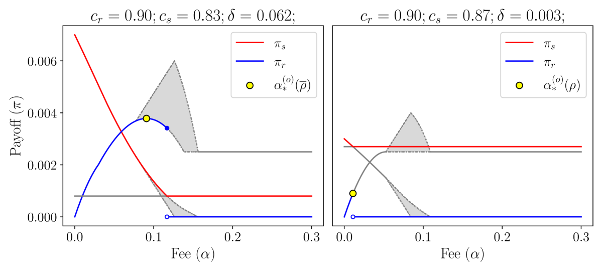
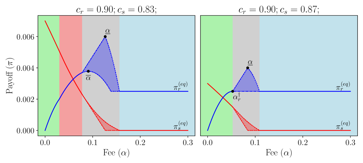
As before, because of the functional dependence of on , this is complicated in general. Just as in Section 5.2, we’ll build intuition by analyzing simpler cases first. In Figure 5, we plot the same equilibrium payoff curves as Figure 4, however we now include an outside option with in the left subplot and in the right subplot. For simplicity, in the left subplot we assume that . If the retailer sets the fee above some threshold, the independent seller would prefer to leave the revenue sharing program and sell on their own instead. It will be helpful to give this threshold a name; let’s define
| (33) |
If the retailer chooses a fee , they will achieve a payoff of in equilibrium of the Outside Option Game because the independent seller will leave. The independent seller, on the other hand, will achieve a payoff of for , which is therefore a lower bound on their equilibrium payoff. Additionally, in equilibrium of the Outside Option Game the retailer will choose a fee , which bounds the maximum fee further away from .
Interestingly, the left subplot of Figure 5 demonstrates that the retailer will not necessarily choose , indeed their payoff under is maximized by choosing . However, if we simply switch the equilibrium strategy profile from to , the retailer will choose , which serves as a good reminder that the choice of may have a significant effect on the equilibrium outcome in general.
The right subplot of Figure 5 shows another interesting case where is low enough such that the independent seller achieves a higher payoff than the retailer in equilibrium. In fact, the independent seller is so competitive with the retailer that the retailer achieves a significantly lower payoff in equilibrium of the Outside Option Game than they would if the indepdendent seller did not exist. Additionally, notice that is not in the continuum region. Because of this, the choice of does not matter, which should be clear graphically because the entire continuum region is “grayed out” for both the retailer and independent seller. In fact, we can say more generally that
| (34) |
which is a simple special case of (32).
The Outside Option Game is the final extension of the shared-revenue Bertrand game that we explore in this paper. The game captures the effect that the cost configurations () and the credibility of the independent seller’s outside option threat () have on the optimal fee structures and the minimum/maximum payoffs achievable in equilibrium of the revenue sharing program.
7. Conclusion and future work
In this work, we presented a game theory model of a shared-revenue Bertrand game to analyze the dynamics and incentives induced by revenue sharing programs. Furthermore, we investigated some natural extensions of the model to make it more realistic by modeling the proportion of revenue sharing as an action and giving the independent seller an outside option to sell on their own. Our findings resonate strongly with existing results from duopolistic competition and optimal taxation theory. In equilibrium, both players are able to achieve positive payoff, and the referral fee is set at a “sweet spot” low enough to stimulate economic activity while high enough to maximize payoff.
However, this work is just a starting point, and there are still many future research directions in which this model can be extended with even more potential implications for understanding the dynamics of revenue sharing:
-
•
To improve the present analysis of the shared-revenue Bertrand game, some natural next steps would be to more completely consider general demand curves and mixed strategies. While we anticipate qualitatively similar equilibria under appropriate assumptions on the demand curves and the mixing distributions, there is much left to formally prove this.
-
•
We have assumed throughout that this is a game of perfect, complete information – modeling uncertainty or forecasting of the costs or demand curves are interesting next steps.
-
•
We do not closely consider the manufacturing of the product, but we would expect the dynamics to differ in the cases that (a) there is one primary manufacturer of the product, from whom both the retailer and indepedent seller buy, or (b) there are many manufacturers of the product, in which case the margins are low.
-
•
We could impose capacity constraints on the players, allowing us to reason about strategies for stocking both retailers’ and independent sellers’ products in the same warehouse.
-
•
We look only at a duopolistic interaction, but more sophisticated models of entry and exit from a shared-revenue Bertrand marketplace may help make the game more realistic.
-
•
A large retailer or ridesharing service may not want to choose a different fee for each individual independent seller on its platform, instead preferring to choose an “aggregate fee” for a homogeneous group of independent sellers.
-
•
Empirical studies of revenue sharing programs could reveal aspects of the real world our models fail to capture, including in the other application domains introduced in Section 1.1.
Ultimately, this work marks an important first step towards understanding cooperative business practices between economic agents from first principles.
Acknowledgements.
We would like to thank Dirk Bergemann for his insightful comments and suggestions.References
- (1)
- Bertrand (1883) Joseph Bertrand. 1883. Review of “Theorie mathematique de la richesse sociale” and of “Recherches sur les principles mathematiques de la theorie des richesses.”. Journal de savants 67 (1883), 499.
- Binmore et al. (1989) Ken Binmore, Avner Shaked, and John Sutton. 1989. An Outside Option Experiment. The Quarterly Journal of Economics 104, 4 (1989), 753–770. http://www.jstor.org/stable/2937866
- Blume (2003) Andreas Blume. 2003. Bertrand without fudge. Economics Letters 78, 2 (2003), 167–168. https://doi.org/10.1016/S0165-1765(02)00217-3
- Chang (2014) Chen-Yu Chang. 2014. Principal-Agent Model of Risk Allocation in Construction Contracts and Its Critique. Journal of Construction Engineering and Management 140, 2, Article 1 (Aug. 2014), 9 pages. https://doi.org/10.1061/(ASCE)CO.1943-7862.0000779
- Coase (1937) R. H. Coase. 1937. The Nature of the Firm. Economica 4, 16 (1937), 386–405. https://doi.org/10.1111/j.1468-0335.1937.tb00002.x arXiv:https://onlinelibrary.wiley.com/doi/pdf/10.1111/j.1468-0335.1937.tb00002.x
- Coats (2002) Jennifer C. Coats. 2002. Applications of Principal-Agent Models to Government Contracting and Accountability Decision Making. International Journal of Public Administration 25, 4 (2002), 441–461. https://doi.org/10.1081/PAD-120013250 arXiv:https://doi.org/10.1081/PAD-120013250
- Demuynck (2019) Thomas Demuynck. 2019. Bertrand competition with asymmetric costs: a solution in pure strategies. Theory and Decision 87, 1 (April 2019), 147–154. https://doi.org/10.1007/s11238-019-09698-4
- Govindan and Wilson (2016) Srihari Govindan and Robert B. Wilson. 2016. Nash Equilibrium, Refinements of. Palgrave Macmillan UK, London, 1–14. https://doi.org/10.1057/978-1-349-95121-5_2515-1
- Kartik (2011) Navin Kartik. 2011. A note on undominated Bertrand equilibria. Economics Letters 111, 2 (2011), 125–126. https://doi.org/10.1016/j.econlet.2011.01.013
- Laffer (2004) Arthur B. Laffer. 2004. The Laffer Curve: Past, Present, and Future. Heritage Foundation 1765 (2004). https://www.heritage.org/taxes/report/the-laffer-curve-past-present-and-future
- Osborne and Rubinstein (1990) M.J. Osborne and A. Rubinstein. 1990. Bargaining and Markets. Academic Press. https://books.google.com/books?id=JaoUAQAAMAAJ
- Rasmusen (1989) Eric Rasmusen. 1989. Games and information. Vol. 13. Basil Blackwell Oxford.
- Stern (1976) N.H. Stern. 1976. On the specification of models of optimum income taxation. Journal of Public Economics 6, 1 (1976), 123–162. https://doi.org/10.1016/0047-2727(76)90044-X
- Stiglitz (1987) Joseph E. Stiglitz. 1987. Chapter 15 Pareto efficient and optimal taxation and the new new welfare economics. In Handbook of Public Economics. Handbook of Public Economics, Vol. 2. Elsevier, 991–1042. https://doi.org/10.1016/S1573-4420(87)80010-1
- Tadelis (2002) Steven Tadelis. 2002. Complexity, Flexibility, and the Make-or-Buy Decision. The American Economic Review 92, 2 (2002), 433–437. http://www.jstor.org/stable/3083446
- Watson (2020) Joel Watson. 2020. On the outside-option principle with one-sided options. Economics Letters 191 (2020), 109110. https://doi.org/10.1016/j.econlet.2020.109110
- Williamson (1975) O.E. Williamson. 1975. Markets and Hierarchies, Analysis and Antitrust Implications: A Study in the Economics of Internal Organization. Free Press. https://books.google.com/books?id=JFi3AAAAIAAJ
Appendix A Notation table
| Notation | Value(s) | Description |
| Marginal cost for player | ||
| Price set by player | ||
| Referral fee | ||
| Market split proportion if prices are equal | ||
| (5) | Quantity demanded for player | |
| Space of price configurations, eg. | ||
| Outcome where player fulfills demand at price | ||
| Additional marginal cost if independent seller leaves | ||
| Equilibrium strategy profile of shared-revenue Bertrand game | ||
| Equilibrium strategy profile with maximum prices | ||
| Equilibrium strategy profile with minimium prices | ||
| Player ’s payoff | ||
| Payoff in equilibrium of shared-revenue Bertrand game | ||
| Payoff in equilibrium of leaving subgame | ||
| Player ’s payoff when fulfills demand at | ||
| Seller optimal feasibility cost; is necessary for to be a potential equilibrium | ||
| Seller optimal single agent price, the maximizer of | ||
| Seller optimal single agent price in leaving subgame | ||
| Retailer optimal single agent price, the maximizer of | ||
| Retailer indifference price, satisfying | ||
| Seller indifference price, which is also their breakeven price as it satisfies | ||
| (12) | Retailer optimality equivalence price, satisfying | |
| (62) | Seller relevance fee, below which selling at becomes a potential best response | |
| Retailer relevance fee, above which allowing the independent seller to sell at becomes a potential best response | ||
| Seller optimal price feasibility fee, above which becomes a potential equilibrium | ||
| Retailer optimal price feasibility fee, above which becomes a potential equilibrium | ||
| Optimality switching fee satisfying | ||
| (28) | Retailer equilibrium alpha in the Fee Optimization Game | |
| See Lemma 4 | Retailer equilibrium fee with strategy profile | |
| Retailer equilibrium fee with strategy profile | ||
| (32) | Retailer equilibrium fee for the Outside Option Game | |
| (33) | Maximum fee for which the independent seller prefers to stay in the revenue sharing program rather than exercise their outside option in the Outside Option Game |
Table LABEL:tab:notation summarizes the symbols used throughout the paper along with their value or range of possible values. We use to denote the retailer and to denote the seller, with placeholders in quantities that are defined analogously for both players. When clear from context throughout the paper, we drop some of the explicit arguments of the functions – note for instance that the prices and fees implicitly depend on the costs.
Appendix B Justification of game setup
B.1. The retailer and seller can achieve nonzero payoff
We assume in Section 2 that . Indeed, suppose on the other hand that . Then, the game becomes trivial:
Lemma 0.
In a shared-revenue Bertrand game with , the only admissible Nash equilibrium is .
Proof.
The retailer’s dominant strategy is setting . Consider a price . If ,
On the other hand, if , we have
With this, the independent seller’s best response is clearly . ∎
Enforcing this requirement allows us to avoid such trivial equilibria where one or both players abstain from the market because they will simply never fulfill demand at any price.
B.2. Independent seller’s cost is lower
We also assume in Section 2 that . Suppose on the other hand that . Then, the game becomes trivial:
Lemma 0.
In a shared-revenue Bertrand game with , there are no Nash equilibria where the independent seller fulfills demand.
Proof.
Suppose for contradiction there exists an equilibrium where the independent seller fulfills demand. Then, we claim the following must be satisfied:
-
(I)
-
(II)
Indeed, to show (I) suppose for contradiction . Then, we have
Similarly, if , we have .
To show (II), suppose for contradiction . Then, by construction of , we have
by continuity of , this implies that there exists some such that , and therefore yields a lower payoff than so the retailer is not best responding.
However, both (I) and (II) cannot be simultaneously satisfied, because under the assumption that we have that
Thus, such an equilibrium cannot exist. ∎
Because we are interested in modeling the dynamics between the retailer and independent seller, if there are no equilibria where the independent seller fulfills demand our model is entirely uninteresting. Intuitively, if the retailer can fulfill demand themselves for less cost per unit, they have no incentive to initiate a revenue sharing program in the first place.
This implies that the revenue sharing program is best thought of as permitting the sale of niche items or services that the retailer does not specialize in. Instead of specializing in this offering themselves, the model aims to find the conditions under which it would be beneficial for the retailer to partner with the specialist independent seller.
Appendix C Proof of Proposition 1
Proposition 0.
Let , with the equilibrium quantities sold by each player and . Then .
Proof.
Let be an equilibrium market price, with the equilibrium quantities sold by each player and , with . Then the total quantity sold is and the retailer’s payoff is
| (35) | ||||
We examine three possible cases — , and — and show that in each case, one of the players has an incentive to deviate to a different price.
If (the retailer’s payoff per unit it sells is larger than its payoff from the independent seller fullfilling that unit), then the retailer prefers to deviate by setting a price to take the entire market. Similarly, if , the retailer can achieve a higher payoff by deviating to price , allowing the the independent seller to fulfill the demand. When , the independent seller’s payoff is . A similar argument, comparing and , shows that the independent seller will either decrease its price to take the entire market, or increase its price and allow the retailer to fulfill the demand (since the independent seller only achieves nonzero payoff when they fulfills demand themselves, this last case will only happen if is below the independent seller’s breakeven price). Note that the case of and is impossible, as that would imply , which contradicts our assumption that . Thus, if , the proposed price and market split does not constitute an equilibrium. ∎
Appendix D Detailed equilibria derivation
This section is dedicated to deriving the Nash equilibria of (22) and (23). For clarity of exposition, we outline conditions that any Nash equilibrium price configuration must satisfy. By definition of a Nash equilibrium, the following must hold:
-
(I)
-
(II)
-
(III)
-
(IV)
D.1. Shared-price equilibria in which the retailer fulfills demand
Condition IV always holds, as the independent seller achieves a payoff of zero whether they set some price or they set price and allow the retailer to fulfill all demand.
Condition I requires the retailer would not prefer to set a price . Because is a concave quadratic function, it is increasing on , so condition I holds if and only if . Indeed, we derive an expression for by differentiating the quadratic and setting it equal to :
| (36) |
Condition II is equivalent to saying that the retailer would not prefer to increase their price, effectively allowing the independent seller to fulfill demand at price instead of the retailer fulfilling demand at price . Formally, we need
| (37) | ||||
Indeed, is defined as the price at which the retailer’s payoff is equal no matter which seller fulfills demand, which is exactly equal to –
| (38) |
With this intuition, the simplification in (37) is almost true by definition. All that is required is to show the direction of the inequality, which is correct because the retailer’s payoff from the independent seller fulfilling demand at is zero, but is negative when it fulfills demand on its own at .
Condition III posits that the independent seller would not prefer to undercut the retailer and fulfill demand themselves at some price . However, recall that in an equilibrium where the retailer fulfills demand, the independent seller achieves a payoff of . Thus, we can rewrite condition III as:
| (39) | ||||
Because is a concave quadratic function, we have that
Where is the maximum of , for which we find a closed-form –
| (40) |
If , then and the condition never holds. On the other hand, if , then (39) reduces to
| (41) | ||||
where we ignored the because . Indeed, we have that because
| (42) |
Combining the conditions, we have shown that an equilibrium price in which the retailer fulfills demand must satisfy . However, because , we have
| (43) |
so the interval is always empty and there exist no equilibria in this case.
D.2. Shared-price equilibria in which the independent seller fulfills demand
Condition II always holds, as the retailer does not fulfill any demand whether they set some price or price and thus achieve the same payoff either way.
Condition III requires that the independent seller would not prefer to fulfill demand at . Because is a concave quadratic function maximized at , condition III is equivalent to .
Condition IV requires that the independent seller would not prefer that the retailer fulfill demand; it simplifies to
| (44) | ||||
Finally, condition I posits that the retailer would not prefer to undercut the independent seller and fulfill demand themselves at some price . Formally, we can rewrite condition I as
Because is a concave quadratic function, we have that
| (45) |
D.2.1. Equilibria where
Consider the first case of (45) where . Condition I then simply becomes , which we showed in (37) is equivalent to . Thus, we have found a continuum of equilibria , so long as the interval is nonempty. Note that and always, so we can drop those.
Conditions under which the interval is nonempty.
We showed in (43) that always, and we have the following condition for –
| (46) |
Where gets its name because is necessary for to be an equilibrium. Furthermore, we can see that is equivalent to the following –
| (47) |
However, this is implied by ; we can see easily that because
| (48) | ||||
This intuitively makes sense, because as we argued in (9), the independent seller cannot attain positive payoff if , so of course in this limit the equilibrium is feasible. Thus the interval of prices is nonempty if and only if .
Conditions under which is the upper bound.
We have the following condition for –
| (49) |
It will become clearer in Appendix D.2.2 where the notation comes from. Furthermore, when
| (50) |
Note that always because
| (51) | ||||
We acknowledge that it is not yet clear when or ; this is a question to which we will return shortly. However, we can conclude for now that is the upper bound when .
Conditions under which is the upper bound.
We see that when
| (52) |
The notation comes from the implication of (52) between optimal prices for retailer and seller. Additionally, per (50), we have that , which is exactly the namesake of . Furthermore, we can see that –
| (53) |
This should once again be intuitive because clearly, could not be an equilibrium if , as the independent seller would prefer to undercut the retailer and sell at instead. Thus, we have that is the upper bound of the interval when , provided the interval is nonempty.
Conditions under which is the upper bound.
Conclusion and summary of equilibria.
Explicitly simplifying the condition is uninsightful, so instead we will break up the equilibria into two cases based on which direction of this inequality is true. However, we will prove one equivalence that will make our presentation easier throughout –
| (54) |
Note we showed in (51) that , so as a corollary of (54), we know that implies that as we wanted before. Finally, for ease of presentation, we will manipulate (54) to find an equivalent condition in terms of and –
| (55) |
To summarize, we have so far found the following equilibria:
Case (i), :
| (56) |
D.2.2. Equilibria where
Now, consider the second case of (45) where . The price at which is equal to was defined in Section 2.2 to be , which is the solution to the following quadratic equation:
| (58) | ||||
Where we choose the larger solution, as the smaller solution satisfies the following inequalities
| (59) |
and therefore drops when we consider that we are handling the case of . Note that, in order for to be well defined, we need the discriminant to be positive which occurs precisely when ; we will return to this later in this subsection. Thus for an equilibrium in this case, we need that . Note that and always, so we can drop those conditions.
From (46), we have that . We won’t explicitly simplify the condition here; we delay that until (76). For now we will simply remark that is maximized at , which follows because
So, because and is a concave quadratic, we have that
| (60) |
We’ll check to make sure that the interval of prices is nonempty in each of the possible cases:
Interval is .
Per (47), we have that . However, we have not found the conditions under which . By the same argument as in (60), we have the following equivalences:
| (61) |
Now, recall that
which implies that is well defined and that . We see upon substituting the endpoint into (61) that
Furthermore, we show in (85) and (86) that has a unique maximum at , which is sufficient to imply that there exists some such that . For completeness, explicitly solving (61) yields the closed-form
| (62) |
Therefore, the interval is feasible as long as .
Interval is .
Interval is .
Interestingly, we find the following condition for :
| (63) |
Thus, is nonempty so long as . Note we showed in (51) that always.
Reconciling equilibria with case (i) where .
We’ve so far shown that or could be an equilibrium if . In (56) and (57), we subdivided the equilibria into two cases, when and . Though we have not explicitly simplified the condition , it would be prudent to consider what equilibria exist when is between and .
More specifically, suppose . We will show here the following claim: for all . Recalling our condition from (60), we have that
In this case, we have
Similarly, we can see that
Thus, to show the claim, all we need to show is that is lower bounded by its value at the endpoints for . We do this by finding the derivative:
| (64) |
Note that the that maximizes (which will appear in the future in Lemma 4 where we show that ) satisfies the following –
Because the function is a bijection from , this importantly implies that has a unique maximum for . Now, we claim that is decreasing at , which follows because –
Which always holds because, as we showed in (54), when we have always. This is sufficient to conclude the proof of the claim. Given the claim, we can now conclude that when , the region of equilibria we have found is , which is the same as we found before. Note that is well defined for all , which is implied by :
| (65) | ||||
Reconciling equilibria with case (ii) where .
Switching the direction of the inequalities in the proof from the previous subsection yields the analogous result that if , for all . We previously found that for all , the equilibria are . However, by the same argument as in (60) we have that
which always holds, thus we have found no new equilibria in this region of parameter space.
Conclusion and summary of equilibria.
Combining with the equilibria from the first case from (56) and (57), we have the following shared-price equilibria where the independent seller fulfills –
Case (i), :
| (66) |
Case (ii), :
| (67) |
D.3. Equilibria where
Condition IV is always satisfied; because for all , , the independent seller achieves a payoff of both at price and price . Together, conditions I and II imply that the retailer must set price so as to maximize their payoff function. Otherwise, if they are not at the optimal price, they would be able to increase their payoff by changing their price.
Furthermore, condition II requires that it is not the retailer would not achieve a higher payoff by deviating to some price so as to let the independent seller fulfill demand in equilibrium. Formally, we need that
However, this is exactly the equation we solved in (58), so we have that must be greater than (recall from (59) that the smaller root is always less than ). Note that we also must have that , and in (63) we showed that is equivalent to .
We move on to condition III now. Recall that for any we have that . Thus, condition III simplifies to
The maximum of the independent seller’s payoff on the interval is attained at
because is maximized at . Consider the second case when . Recall from (9) that
Thus, we find immediately that when , condition III never holds if and always holds if . However, if , we have that , which is a contradiction. Thus there are no equilibria where .
On the other hand, if , which we showed in (52) is equivalent to . With this, condition III is satisfied in this case if
| (68) | ||||
| (69) |
As a remark, see that (68) can be rewritten as , which is obvious in hindsight because is by construction the price below which the independent seller makes nonpositive payoff. We showed in (51) that , so is sufficient to imply that per (63). Additionally, recall from (53) that .
In summary, we have a continuum of equilibria whenever .
D.4. Equilibria where
In this case, condition II is always satisfied; the retailer does not fulfill any demand either way as, for all , . As in the previous case, conditions III and IV together imply that the independent seller must set price . Condition IV requires that the independent seller does not prefer to let the retailer fulfill demand in equilibrium, in which case they would earn a payoff of . To satisfy this, we need only that the independent seller sets a price , which always holds for price .
Thus, all that remans to check is condition I. Simplifying the condition, we need that
Once again, there are two cases for the choice of that maximizes the retailer’s payoff function on the interval –
Consider the second case where . From (52), recall that . Recalling our analysis from (60), condition I then simplifies to
Note that by construction of , thus is necessary for condition I to hold. Thus, we have a continuum of equilibria whenever and holds. Additionally, recall that if , we showed above that can only hold when .
Now consider the first case where . From (52), recall that . On the other hand, we have that condition I becomes
Thus, we have a continuum of equilibria whenever . Note that it’s not always the case that , but when this holds, such equilibria exist. Additionally, it’s clear that always.
Appendix E Refining and interpreting equilibria - proofs
E.1. Admissibility
For the independent seller, playing is weakly dominated by playing a price , because their payoffs are equal if the retailer sets a price but for we have
because they achieve negative payoff when fulfilling demand below their breakeven price. Playing a price is dominated by playing because, for all ,
where the inequality holds because . For any price , we have
which implies weak dominance as desired. However, consider for instance two prices , we claim neither dominates the other. If ,
because . On the other hand if ,
Thus, in any region of parameter space, the only admissible strategies for the independent seller are , except for a technical edge case when which we will address later.
A similar result holds for the retailer, except it’s not always the case that (which occurs precisely when per (49)). We claim that dominates all . Indeed, for , the retailer’s payoff is the same. For , the retailer’s payoff is
where the inequality holds because . For , we have
where the inequality holds because .
Similarly, dominates all . Indeed, for , the retailer’s payoff is the same. For , the retailer’s payoff is
where the inequality holds because . For , we have
where the inequality holds because . However, we can show fairly easily that for any , neither weakly dominates the other. Suppose , then for we have
because . While, for, , we have
because . Reversing the directions of the inequalities proves that there are no dominant strategies for any .
With this in mind, we will step through each of the Nash equilibria that we found in (66) and (67) and remove those strategies that are weakly dominated.
First consider an equilibrium in the regime where . Here, the Nash equilibrium is . Because the retailer’s admissible strategies fall in the interval , the only admissible equilibrium price is .
Now, suppose that , in which case the Nash equilibria are . We showed that in this region of parameter space, we have . Notably, this implies that the entire continuum of shared-price equilibria are inadmissible because it is entirely disjoint from the admissible region for the retailer, . Thus, the admissible equilibria are if and if .
Now, suppose and . As before, the Nash equlibria are . However, this time, we have . Here, the retailer’s admissible prices are , so the remaining admissible equilibria are .
The arguments of the previous paragraph did not depend on the relative ordering of and , and we know that per (63) because . Thus the admissible equilibria when and are simply the shared prices .
Consider the case when , where the equilibria are . In this case, always. If also, then the only admissible equilibria are as prices are inadmissible. On the other hand, if , the admissible equilibria are .
Now suppose that , here the only Nash equilibrium is . In this region of parameter space, we always have that by construction of , so the admissible Nash equilibria are .
However, when , we have that and the Nash equilibrium is again given by . In this limit, setting weakly dominates setting any because which implies that the independent seller would achieve negative payoff for each unit sold at price and would prefer to achieve 0 payoff by setting . Thus, the only admissible equilibrium when is . Note that this edge case is technical and unimportant, as no matter what price the independent seller sets, the result remains the same – when is high, there is an equilibrium where the retailer fulfills demand.
Summarizing, we have narrowed our focus to the following admissible equilibria:
Shared equilibria, irrespective of ordering of and :
| (70) |
Case (i), :
| (71) |
Case (ii), :
| (72) |
E.2. Relative Pareto optimality
Consider the equilibria in (70), (71), and (72), we will remove any that are Pareto suboptimal relative to other admissible Nash equilibria. There is one Pareto-suboptimal admissible equilibrium (indicated in the first case of (70) by Footnote 8), when and , in which case the retailer fulfilling demand at yields them the same payoff as the independent seller fulfilling demand at . However, the latter earns the independent seller positive payoff while the former earns the independent seller a payoff of . Thus, the equilibrium is Pareto suboptimal relative to the shared-price equilibrium .
When or , there is only one admissible equilibrium. When , despite there being a continuum of equilibria in some of these cases, they all result in the same outcome with the retailer fulfilling demand at . Similarly, when , all of the equilibria result in the independent seller fulfilling demand at . In the remaining cases, all equilibria are Pareto optimal, because the retailer prefers to push the price lower towards and/or (their optimal price when the independent seller fulfills demand) and the independent seller prefers to push the price higher towards .
Appendix F Optimizing the referral fee - proofs
F.1. Nash equilibrium refinements
First, we justify the claims made in Section 5 about relative Pareto optimality and admissibility of equilibrium strategies for the sequential game.
Suppose there are two Nash equilibria of the sequential game and with . Because these are both equilibria, they must have the same payoff to the retailer. However, because the independent seller’s payoff is monotonically decreasing in , is less Pareto optimal than . Thus, Pareto optimality yields us the natural refinement that the retailer will choose the minimum necessary to attain their maximum possible equilibrium payoff.
Let , we will produce a strategy for the independent seller in which the retailer achieves a higher payoff with and another strategy in which the retailer achieves a higher payoff with . Consider the strategy: “choose price if , otherwise choose price ” where are chosen such that . Switching the strategy to play when and otherwise concludes the proof that both are admissible.
F.2. Investigating equilibrium strategy profiles
Despite the preponderance of possible equilibrium strategy profiles, examining (26) and (27) shows there are only a few possible admissible, Pareto optimal outcomes in terms of who fulfills demand and what price they set. The only region of parameter space in which really matters is when , because in this case there are a continuum of prices at which the independent seller could fulfill demand in equilibrium. Intuitively, this means that though could be very complicated in general, this is the only region in which this generality actually has an effect on the payoffs and the real-world outcomes.
We’ll denote as the equilibrium payoff function for the retailer with strategy and the analogous function for the independent seller. With this notation, we then have , and our eventual goal is to compute this . Even with held constant these are still complicated piecewise functions of , so as a first step we will prove continuity of the equilibrium payoffs in .
Proposition 0.
For all that are continuous on ,999Throughout this paper we consider only pure strategies. However, consider for a moment mixed strategies such that for each , is a valid density over equilibrium prices. Then, the analysis easily generalizes if we define . and are continuous in .
Proof.
Examine the equilibrium prices in (26) and (27). Within each of the pieces of the function, are constant as there is only one price at which demand will be fulfilled in equilibrium, except for when . In this interval, we have
because is continuous in on this interval by assumption and are continuous functions of the price , this is a composition of continuous functions which is continuous.
Thus, all that remains to check is that at each of the transitions between pieces, the lower limit is the same as the upper limit of and . We showed in (50) that when . However, the remaining transitions are not quite as clear, as they depend on the value of when and . We will handle each of these cases in turn.
Now suppose that . When , we showed in (63) that (and for ). Because yields an admissible, Pareto optimal equilibrium price configuration for each and is continous, the squeeze theorem tells us that
| (73) |
Furthermore, we showed in (49) that at , , implying continuity because
| (74) |
A similar application of the squeeze theorem shows continuity in when as , because we showed in (52) that .
We know by construction that is the referral fee at which . Because was defined satisfy , and above the equlibrium outcome is the retailer fulfulling demand at , we can apply the squeeze theorem a final time similar to show continuity as . ∎
Corollary 0.
For , let and . Then, , and .
Proof.
Because is an equilibrium strategy profile, we know that for all , . However, note that is the maximizer of the concave quadratic and is the maximizer of the concave quadratic . Thus, for any given , the retailer achieves their maximum (minimum) payoff by choosing the lowest (highest) possible equilibrium price and the independent seller achieves their maximum (minimum) payoff by choosing the highest (lowest) possible equilibrium price. ∎
F.3. Lower bounding the retailer’s payoff
Following the argument from Corollary 2, we know given , the retailer’s payoff is minimized at the maximum possible price. In other words, the worst-case would be one that always chooses the maximum possible price when there are multiple equilibrium prices, precisely for . Formally, for all , we have
Thus, we turn our attention to maximizing the retailer’s equilibrium payoff in the worst case with . First, we show the maximizer of is never in a piece where the independent seller fulfills demand at , because the retailer’s equilibrium payoff is never greater than their payoff when setting the fee above and fulfilling demand themselves.
Lemma 0.
Proof.
First, let’s find the derivative of :
Notice that for all , and that there is a maximum exactly when . Substituting this value into , we find that
∎
Because we are working with , the only remaining equilibrium outcomes that could maximize the retailer’s payoff are ones where the independent seller fulfills demand at or and one where the retailer fulfills demand at . However, by construction . Thus, all that remains is to understand if or when the retailer can achieve a greater payoff than in an equilibrium where the independent seller fulfills demand at .
To this end, we will first find the that maximizes , temporarily ignoring the question of if that is actually an equilibrium where is observed, which will be addressed separately in Lemma 5.
Lemma 0.
The maximizer of is .
Proof.
We found the derivative of in (64). Setting the expression equal to , we find that the critical value must satisfy
| (75) |
We will explicitly solve the cubic (75) for . As an important remark that is worth restating, the function is a bijection from , so is the unique value that satisfies (64) for . To obtain our explicit solution, we first write it in standard form:
We perform the change of variables to obtain a depressed cubic:
Using Cardano’s formula to solve the depressed cubic, we find that the real root is
as desired. Note that the discriminant is positive, so is indeed always real. ∎
Note that if there exists any such that , then also satisfies . This follows because is a concave quadratic maximized at for all , and because , we have
| (76) |
Before proceeding, we’ll pause to build some intuition about when this condition holds.
Remark 1.
If , always.
Proof.
The proof of Remark 1 breaks down when because we have now that . When , there sometimes exists an satisfying (76) and sometimes does not. With this, we can now answer the question of if this maximum payoff is actually attainable in equilibrium.
Lemma 0.
If , then .
Proof.
To prove the upper bound, suppose for contradiction that . Then, by construction of and (76), we have a contradiction because
For the lower bound, we prove a stronger statement. First, note that for all ,
| (78) |
We claim that, for all ,
| (79) |
Combining (79) with (76), (77), (78) is sufficient to conclude the proof because
Thus, all that remains is to show (79). Manipulating the inequality, we have
| (80) | ||||
| (81) |
To minimize the left side, we first take the derivative with respect to to find the critical –
Thus, the left side of (81) is lower bounded by its value at . We will show that (80) holds with equality for , which is sufficient to conclude the proof. Indeed, for the left side we have
and for the right side we have
∎
With this, we have shown that if the retailer chooses , yields an equilibrium strategy profile in which the independent seller fulfills demand at price . This is sufficient to conclude that:
| (82) |
We have shown that in the first case and otherwise. Ideally, we would be able to directly translate this to a tight bound on for all in the first case, however it is still possible that there exists some and some such that
| (83) |
For instance, (83) could hold if for some well-chosen , but for all other , we set . If we impose some assumptions on the functional form of , we may be able to translate (82) into a tighter bound on . However, we do not investigate further tightening the bound in this work as we have at least shown that the lower bound is tight whenever we are in the second case of (82).
With this, the maximum payoff that the independent seller could achieve in equilibrium of the sequential game is either by fulfilling demand at or . If it is at , clearly they would prefer the lowest possible . If it is at for some , we have
This leaves us with the result that the independent seller’s payoff in equilibrium of the sequential game is bounded by
which is loose for similar reasons as our bound on .
F.4. Upper bounding the retailer’s payoff
Analogous to the previous subsection, we know that the upper bound for the retailer’s payoff will be with the strategy profile . The retailer’s maximum payoff either occurs when the independent seller fulfills demand at or , or when the retailer fulfills demand themselves at . Recall that per (46). The retailer’s payoff function when the independent seller fulfills at is simple –
This is clearly increasing in , so the maximum payoff that the retailer could achieve when the independent seller fulfills at is by setting . At this , we have
| (84) |
Notice that this yields a higher payoff than the retailer fulfilling demand on their own, because
Finally, it remains to see if the retailer could achieve a higher payoff than (84) for at price . The payoff function is slightly less simple –
it’s not obvious if this is increasing or decreasing in , so we will take the derivative:
| (85) |
Clearly, the unique maximum occurs when , and is decreasing in for . However, we have that
| (86) | ||||
Thus, the maximum equilibrium payoff the retailer can attain when the retailer sells at is at the minimum possible , which is in fact . Conventiently, this implies that the maximizer of the retailer’s payoff function with the strategy is precisely . Because at , we have , this is sufficient to conclude that
Just as the previous case, this is unfortunately not sufficient to conclude that in general; the best we can do is conclude that . For the independent seller, it proves the trivial bound that , where the bound is tight because when and , the independent seller is fulfilling demand at and achieves a payoff of .
Appendix G Equilibria of leaving subgame
The leaving subgame is simply a standard Bertrand game with asymmetric costs . Though this has been derived in the literature for general demand curves such as in (Blume, 2003; Kartik, 2011), for completeness we include here a brief derivation of the equilibria contextualized to our setting. First, note that , which follows as a corollary of Proposition 1 when . Thus, any shared-price equilibrium must have exactly one player fulfill demand. However, we have that
Lemma 0.
In all Nash equilibria of the leaving subgame, the independent seller fulfills demand.
Proof.
Suppose for contradiction there exists such an equilibrium . Clearly, we must have , otherwise at a price the retailer would prefer to increase their price to and achieve a payoff of rather than achieving negative payoff for each unit sold at . However, this implies that , so setting any price yields the independent seller a payoff of
∎
With this, consider an equilibrium in which the independent seller fulfills demand. In order for this to be an equilibrium, we must have that
However, because a concave quadratic maximized at , it follows that the equilibrium is given by
Consider the first case where . If , because is increasing for , the independent seller achieves a higher payoff by setting price for some . We therefore must have a shared price in this case. If , the retailer achieves a higher price by setting and fulfilling some demand, yielding them a nonzero payoff. Furthermore, if , the independent seller would prefer to fulfill at their optimal price instead. Thus, we have shared-price Nash equilibria at .
Now consider the second case where . If , our analysis reduces to that of the previous case. If, on the other hand, , then we still have similar shared-price equilibria . However, we also gain unequal-price Nash equilibria – the independent seller would no longer benefit from deviating to a price and the retailer still would not prefer to undercut the independent seller because .
To summarize, we have found the following Nash equilibria:
Now that we have found the Nash equilibria, we apply the admissibility refinement that we have been using throughout. Very similar analysis to Appendix E.1 shows that the admissible strategy sets for the retailer and seller are and . While the independent seller is not playing any dominated strategies in equilibrium, the retailer is, so this is a nontrivial refinement. The admissible Nash equilibria are:
From here, we find that the admissible Nash equilibrium outcomes are:
or simply .