∎
Tel.: +8613466749513
22email: tonghs08@mails.tsinghua.edu.cn
A shrinkage probability hypothesis density filter for multitarget tracking
Abstract
In radar systems, tracking targets in low signal-to-noise ratio (SNR) environments is a very important task. There are some algorithms designed for multitarget tracking. Their performances, however, are not satisfactory in low SNR environments. Track-before-detect (TBD) algorithms have been developed as a class of improved methods for tracking in low SNR environments. However, multitarget TBD is still an open issue. In this paper, multitarget TBD measurements are modeled, and a highly efficient filter in the framework of finite set statistics (FISST) is designed. Then, the probability hypothesis density (PHD) filter is applied to multitarget TBD. Indeed, to solve the problem of the target and noise not being separated correctly when the SNR is low, a shrinkage-PHD filter is derived, and the optimal parameter for shrinkage operation is obtained by certain optimization procedures. Through simulation results, it is shown that our method can track targets with high accuracy by taking advantage of shrinkage operations.
Keywords:
Multi-target tracking Track-before-detect PHD filter1 Introduction
In order to extract target measurements, traditional tracking methods apply a detection threshold at every scan. The undesirable effect of detecting the sensor data, however, is that in restricting the data flow, it also throws away potentially useful information. For high signal-to-noise ratio (SNR) targets, this loss of information is of little concern Ref1 . For low SNR targets, this loss of information could be critical for a radar tracking system. Therefore, some new algorithms using unthresholded data are more advantageous than the traditional methods in tracking low SNR targets.
The concept of simultaneous detection and tracking using unthresholded data is known in literature as track-before-detect (TBD) approach Ref1 . TBD algorithms could improve the performance of a tracking system, which has been investigated for surveillance radar Ref2 . In Ref3 and Ref4 , the advantage of TBD methods is discussed and many TBD methods are reviewed and compared. As a batch algorithm using the Hough transform Ref5 , dynamic programming Ref6 or maximum likelihood estimation Ref7 , TBD could be implemented. These techniques operate on several data scans and in general require large computational resources Ref1 .
As an alternative, recursive TBD method is based on a recursive single-target Bayes filter Ref1 . An extension of the particle filter to multitarget TBD is given in Ref8 , and an improved approach is given in Ref9 . In this algorithm, a modeling setup is applied to accommodate the varying number of targets. Then a multiple model Sequential Monte Carlo based TBD approach is used to solve the problem conditioned on the model, i.e., the number of targets Ref10 . This approach has proven to be very efficient in both single and multitarget case Ref3 , though it restricts itself to the case in which the maximum possible number of targets is limited and known.
Another extension of the single-target Bayes filter to multitarget TBD is based on a multitarget Bayes filter. Because a single-target Bayes filter is optimal for a single target, to solve the problems introduced by multiple targets, the multitarget Bayes filter is proposed in Ref11 . In a multitarget Bayes filter, multitarget states and observations are modeled as random finite sets (RFS). This approach is a theoretically optimal approach to multitarget tracking in the framework of finite set statistics (FISST) Ref12 . However, the multitarget Bayes filter has no practical utility without an approximation strategy. To solve this problem, the probability hypothesis density (PHD) filter Ref13 is proposed as a tractable and calculation-simple alternative to the multitarget Bayes filter Ref14 .
The PHD is the first moment of the multitarget posterior probability. Under some assumptions (e.g. Possion Assumption), the PHD is an approximation of the multitarget posterior probability. Therefore, the PHD filter can be an approximation of the multitarget Bayes filter. Although a PHD algorithm for TBD is proposed in Ref10 , this approach ignores TBD measurements should be modeled by RFSs. In Ref15 , multitarget TBD from image observations is formulated in a Bayesian framework by modeling the collection of states as a Multi-Bernoulli RFS. This work use the multi-Bernoulli update to develop a high precision multi-object filtering algorithm for image observations, although its adaptability of low SNR environment is needed to discussed in more detail.
In our previous work Ref16 , we use the RFSs to model multitarget TBD measurements and the collection of states. In this way, a traditional PHD filter Ref12 and Ref13 could be applied to multitarget TBD. Even though PHD could be an approximation of the multitarget posterior probability, the accuracy of the algorithm is limited by some reasons, which are indicated in this paper. Firstly, when the SNR is too low, the PHD cannot be a sufficient approximation of the multitarget posterior probability because the fundamental assumptions are challenged. Furthermore, for multitarget TBD, the measurements of target and noise can hardly be separated, while the PHD filter is heavily dependent on the measurements of targets Ref18 . In traditional tracking systems, to solve these problems, cardinalized PHD filter (CPHDF) is proposed in Ref19 . However, CPHDF is inefficient in multitarget TBD, because the computational complexity of CPHDF is , where is the number of elements of the measurement set and is quite large for the TBD problem.
In this paper, for extending a traditional PHD filter to be suitable for multitarget TBD, viewed from a different perspective, TBD can be regarded as a kind of classification problem of target and noise measurements. To enhance the difference between the target and noise measurements and to pursue better classification performance, the measurements need to be denoised. The threshold shrinkage algorithm Ref20 is an important method for image denoising. In general, the key points of threshold shrinkage are the following: the method of shrinkage (e.g., soft-threshold method) and the selection criterion of the threshold. In this paper, a shrinkage operation is adopted that is similar to the threshold shrinkage algorithm. The optimal parameter for the shrinkage operation can be obtained via certain optimization procedures.
Furthermore, in this paper, some problems of multitarget TBD in particle use are also discussed. The assumption of known SNRs is used frequently in traditional TBD algorithms Ref6 , Ref8 and Ref9 . Multiple targets with similar SNRs are common assumption in the simulations of PHD algorithms using the amplitude feature, as in Ref15 and Ref21 . However, in practical use, multiple targets with different or unknown SNRs are common. In this paper, for the SMC implement of the PHD filter adopted, this problem could be solved by augmenting the SNR into target state, varying the method of generating predicted particles and adjusting the update operator.
In this paper, the measurement of targets is modeled by a ’nail-like’ model on range-Doppler maps because of the assumptions of the classical PHD filter in the framework of FISST. Recently, a classical PHD filter has been modified to solve the problems of extended and group targets in Ref22 and Ref23 , respectively. Therefore, the TBD measurement model of extended targets in the framework of FISST will be discussed in future work.
The rest of this paper is organized as follows. In Section 2, the multitarget TBD problem is modeled by RFSs. In Section 3, the limitation of traditional PHD filter extension to TBD is investigated. In Section 4, a shrinkage option for the PHD filter is proposed with an optimal parameter. Tracking multiple targets with different or unknown SNRs is discussed in Section 5. Simulation results for the tracking system are presented in Section 6. Finally, we conclude the paper in Section 7.
2 Multitarget TBD RFS model
2.1 State of the RFS model
The target state is ,where and are the position and velocity. Since there is no ordering on the respective collections of all target states, they can be naturally represented as a finite set. is the multitarget state-set at time step , i.e., the set of unknown target states (which are also of unknown number).
In a single-target scenario, the state is modeled as random vectors. Then, the multitarget state, including target motion, birth, spawning, can be described by RFS. For target motion, given multitarget state set , each either survives at time step with probability , and its transition probability density from to is . Therefore, the target motion is modeled as the RFS . In the same way, when the RFS of target birth at time is modeled by , and the RFS of targets spawning from a target with is modeled by , the multitarget stat is given by
| (1) |
2.2 Measurement of the RFS model
The measurements are measurements of reflected power as in Ref8 . is white complex Gaussian noise with variance . In this section, assume that the intensity of all targets is , the SNR for the targets is defined by
| (2) |
The method to deal with multiple targets with different or unknown SNRs is discussed in section 5.
Because of the assumptions made in the modeling process and the essential difference between an RFS and a random vector, the two conditions that should be satisfied to model TBD measurements by a RFS are the following: there is no target that generates more than one measurement vector, and no measurement vector is generated by more than one targetRef22 . In summary, the measurement of targets should be modeled by a ’nail-like’ model on the range-Doppler-Bearing maps (the cell is defined by coordinat ()) as follow:
R, D and B are the size of a range, the Doppler and the bearing cell. , and . , and .
Then the measurement model is
| (3) |
| (4) |
This means the measurement of a target is like a nail on the range-Doppler-bearing maps. This ’nail-like’ model is similar to the point target model in Ref5 and Ref6 . At step k, the measurement provided by the sensor consists of measurements , where , and are the number of range, Doppler and bearing cells.
The number of is a constant . However, the number of element of an RFS should be random and Poisson distributed for a PHD filter. Because weak signal information should be preserved by TBD algorithms, we should make sure all measurements produced by targets are included in the RFS. Therefore, a threshold could be chosen as follows:
| (5) |
where the likelihood function for the target is
| (6) |
and that for noise is
| (7) |
where is the zero order Bessel function and is assumed positive.The is the probability detection. Because this algorithm is for TBD, it should be ensured that .
is the observation-set consisting of all measurements collected by all sensors at time-step , no matter the measurement from the targets or from the noise. If , let . Then, the measurement RFS is constructed by a subset of the using a thresholding mechanism. The threshold can insure that by (5). The threshold is a function of the SNR of the targets. The element in the RFS is as follows:
| (8) |
and the likelihood function according
| (9) |
| (10) |
At the same time, the sensor could be modeled by
| (11) |
where the measurements of targets are modeled by RFS and the noise is modeled as RFS . The elements in are the measurements produced by the targets. The elements in are the measurements which are produced by the noise and bigger than as well. It is shown that when the measurements of TBD are modeled by RFSs, multitarget TBD can be regarded as a kind of classification problem of target and noise measurements for one scan. This classification problem will be further analyzed in Section 4.
3 The traditional PHD filter extension to TBD
After multitarget TBD measurements and the collection of states are modeled by RFS, a traditional PHD filter is applied to multitarget TBD. This algorithm is reviewed in 3.1. However, the accuracy of the algorithm is limited by some reasons when the SNR is low, which is discussed in Section 3.2.
3.1 The algorithm
As proposed in Ref13 , the PHD prediction and update equations are presented as follows:
| (12) |
| (13) |
where the PHD is the density whose integral on any region S of state space is . and denotes the intensity of and at time , and is the intensity of . is the time-sequence of observation-sets.
Because the PHD propagation equations involve multiple integrals that have no computationally tractable closed form expressions, Sequential Monte Carlo (SMC) methods are used to approximate the PHD in Ref12 . Let the update PHD at step be represented by a set of particles , as
| (14) |
The predicted particles are generated by
| (15) |
where and are proposal density. The predicted density is
| (16) |
where
| (17) |
Set , the update density will be
| (18) |
where
| (19) |
According to the standard treatment of particle filter, resample to get
3.2 The limitation
Because can be presented by the number of noise samples multiplying the clutter probability density, the update operator (19) turns into
| (20) |
| (21) |
Equation (21) is the likelihood function for the measurement of noise in the measurements set, which denotes the clutter probability density in theoretical filtering (Ref12 and Ref13 ), and the optimal choice of should be the variance of noise , as shown in (20). However, for TBD applications, the SNR is extremely low. Hence, this setting of leads to the situation in which measurements generated by the target and noise are not separated correctly and heavy degradation of tracking performance is seen. In fact, the derivation of (20) depends on the hypothesis that the number of noise sample is Poisson distributed. This means the clutter follows a Poisson distribution and is independent of target-originated measurements. In this way, the PHD can be the ”best fit” approximations of the multitarget posterior probability Ref13 . The average number of noise samples included in RFS is
| (22) |
When is large and is relatively small, the Poisson distribution could be approximated by the distribution of a number of noise samples. However, this approximation will be destroyed when become sufficiently large, which is the case in low SNR scenarios, as in Table 1.
| SNR(dB) | 6 | 7 | 8 | 9 | 10 |
|---|---|---|---|---|---|
| 1340 | 1098 | 707 | 344 | 143 |
When in (20) cannot make PHD a sufficient approximation of the multitarget posterior probability, choosing the ”optimal” becomes the key problem for extending the PHD filter to be applied in TBD. As discussed in the following section, this selection can be considered as a shrinkage operation, and the optimal parameter for the shrinkage operation can be obtained via certain optimization procedures.
4 Shrinkage operation for TBD
To determine the ”optimal” and make the noise and targets distinguishable, a different perspective should be taken. As referred to in Section 2.2, TBD can be regarded as a kind of classification problem for target and noise measurements. In other words, when a measurement is obtained, should it be classified into a target class or a noise class? To solve this problem, the Fisher class separability criterion, as a supplement of to the traditional Bayesian framework, was adopted in our design for the extension of the PHD filter. Furthermore, to enhance the difference between the target and noise measurements and pursue the better performance of classification, some attempts to reduce the noise are needed. The threshold shrinkage algorithm Ref20 is an important method for the image denoising. In general, the cores of threshold shrinkage are as follows: the method of shrinkage and the selection criterion of the threshold. A shrinkage operation is adopted in this section that is similar to the threshold shrinkage algorithm to some extent. The optimal parameter for the shrinkage operation, which acts as the threshold, can be obtained via certain optimization procedures. The PHD filter with the shrinkage operation is called the Shrinkage-PHD filter.
4.1 Fisher class separability criterion
It is known that the Bayesian classifier is the optimal classifier when the posterior probability can be calculated. However, as indicated in Section 3.2, the PHD cannot be a sufficient approximation of multitarget posterior probability when the SNR of the targets is low. Therefore, another classification criterion, the Fisher class separability criterion, is introduced into our methods.
The separation between the two classes of objects defined by Fisher is the ratio of the distance between the centers of classes to the scattering of the classes Ref24 :
| (23) |
where represents the centers of classes and denotes the scattering of the classes. In our analysis, they are set to the mean and variance of the likelihood functions of the target and the noise, respectively.
For targets, the mean and variance are defined as follows:
| (24) |
| (25) |
For the noise, the mean and variance are given by
| (26) |
| (27) |
Therefore, the Fisher class separability is
| (28) |
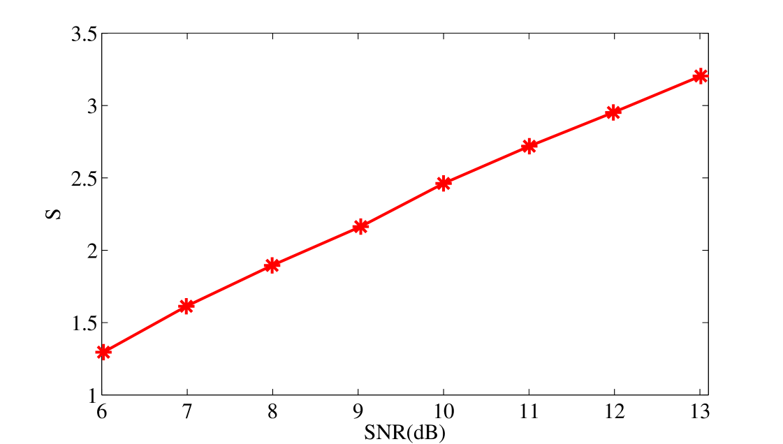
Simulations indicated that the correlation between and the SNR of the targets is a positive, approximately linear relationship (as shown in Fig.1). Therefore, when the SNR is low, the Fisher class separability is so small that the targets and false alarms could not be distinguished. In other words, we should enlarge the Fisher class separability of the target class and the noise class when the SNR of the targets is low.
4.2 Shrinkage operation
To enlarge the Fisher class separability between targets and noise, some kind of ”shrinkage” operation is applied to the likelihood function of the noise. That is, the parameter in (26) and (27) is adjusted. If is chosen instead of itself, then Fisher class separability becomes
| (29) |
Obviously, is larger than whenever . The following question naturally arises: how does one choose the ”optimal” , which is the key parameter for the shrinkage process?
4.3 The optimal parameter for the shrinkage operation
To demonstrate how influences the classification problem of target and noise measurements, we can define the Mahalanobis distance Ref24 of measurement using the center of the noise class and the target class, respectively:
| (30) |
and
| (31) |
Because the selection of the threshold is a difficult task for the threshold shrinkage algorithm Ref20 in the field of image denoising, the selection of the optimal parameter for the shrinkage-PHD filter involves similar problems. For the threshold shrinkage algorithm, an oversized threshold may result in the loss of signal. In contrast, too much noise may remain if an undersized threshold is used. In the same way, for the shrinkage-PHD filter, preserving the weak target information and reducing the noise by tracking are the major challenges to be addressed for TBD problems. Therefore, when considering the two sides, the selection criterion should be designed as follows:
| (32) |
The first constraint represents the ”shrinkage”. To preserve the weak target information and classify as many low SNR targets to the target class as possible, the Mahalanobis distance of measurement with the center of noise class should be enhanced; hence, the variance of the noise class should be reduced.
The second constraint refers to the fixed probability of target loss. The reason for this term is that for TBD problems, false alarms can be reduced by integration over time. Meanwhile, if target loss occurred, the integration of the information of targets is broken off. Hence, the cost of target loss is much larger than the cost of false alarms, which is the main difference between TBD and common radar detection. Moreover, for the PHD filter, a missed detection can result in loss of the track Ref18 . Therefore, target loss should be fixed as . When the is set, a critical value is determined.
The third constraint means that the measurements determined by the second constraint should be classified as targets. When the SNR is low, always intersects , so the optimal solution to (32) is deduced, as indicated in Fig.2(a). With the increasing SNR, becomes much larger than and thus we choose , as shown in Fig.2(b).
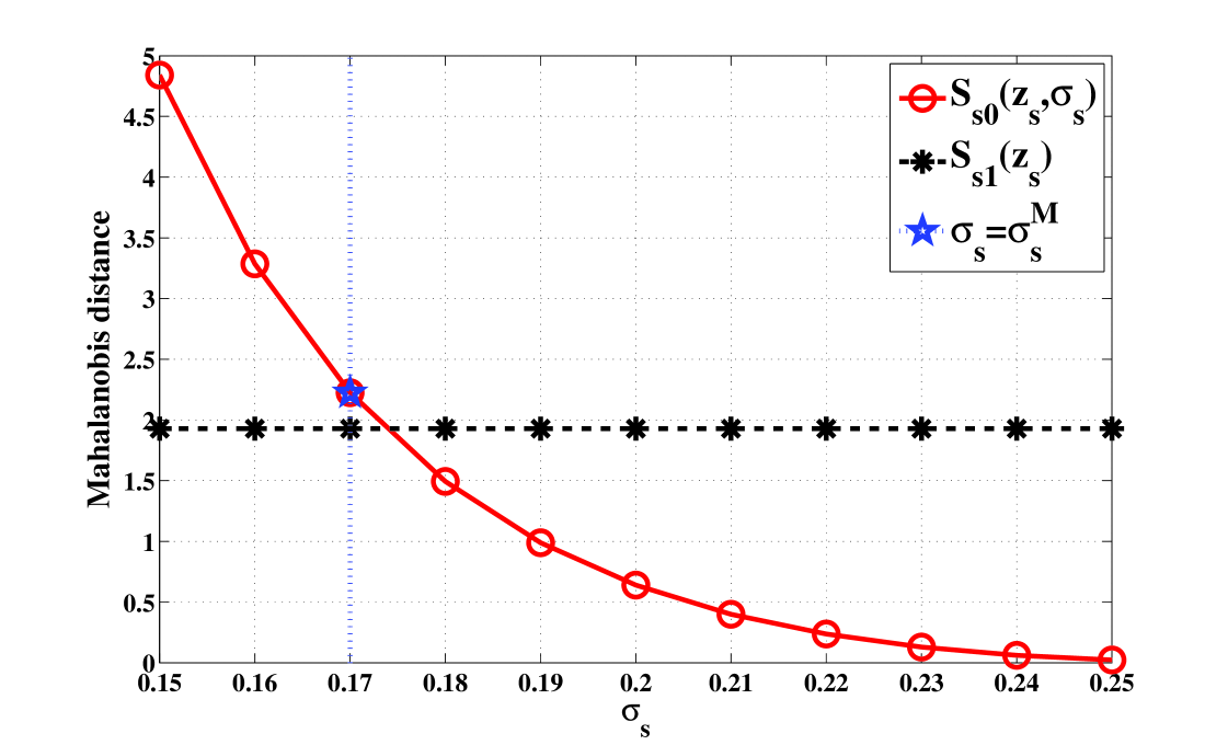 |
| (a)SNR=8dB |
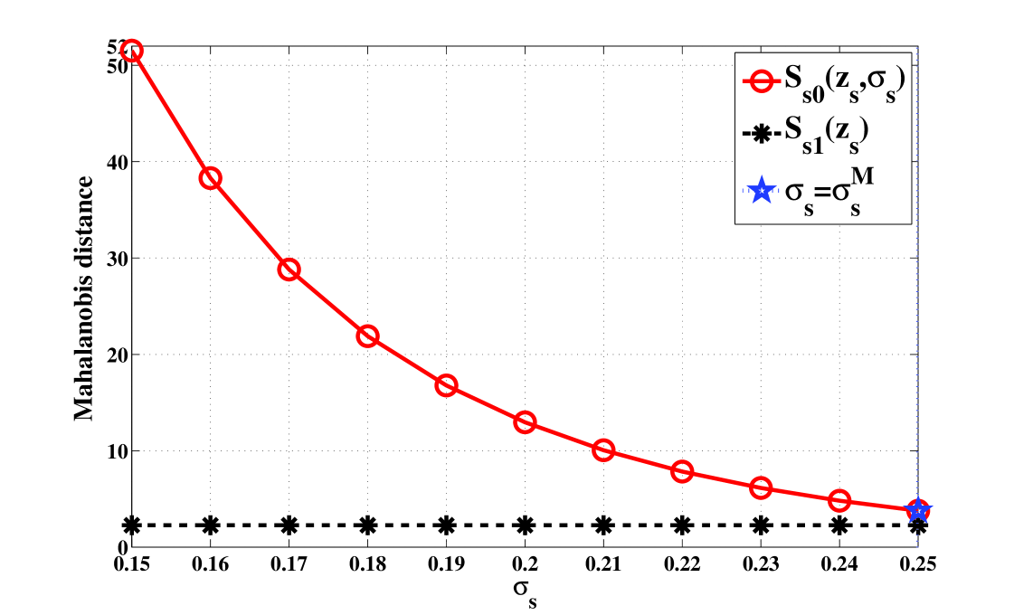 |
| (b)SNR=13dB |
Note that although the shrinkage operation could highlight the target measurement and reduce the possibility of losing the target during tracking, the noise might be incorrectly increased unavoidably. To minimize the influence of shrinkage on the classification of the noise measurement, the maximum , which is consistent with the above constraints, is obtained. The optimal solutions to (32) under different SNRs are listed in Table 2:
| SNR(dB) | 6 | 7 | 8 | 9 |
|---|---|---|---|---|
| SNR(dB) | 10 | 11 | 12 | 13 |
The update operator of the shrinkage-PHD filter can be summarized as follows:
| (33) |
where should be set according to Table 2.
5 Multitarget TBD in practical use
This section is to solve of the problem of tracking multiple targets with different or unknown SNRs.
As proposed in Section 4, the optimal parameter for the shrinkage operation is closely related to the SNRs of the target, and the SNRs of the target are assumed to be known and similar. However, in practical use, multiple targets with different or unknown SNRs are common. The PHD is the first moment of the multitarget posterior probability, but not the posterior probability of a certain target. Therefore, the in (6) and the in Table 2 are difficult to determine. Because the SMC implement of the PHD filter is adopted, this problem could be solved by adjusting the method of generating predicted particles and the update operator.
To describe how to deal with the different SNRs of multiple targets, we augment into :
| (34) |
where . The particle of the target state is . The is generated as (15)
| (35) |
The is generated by the assumption of a uniform distribution in the range of , where the SNRs of all of the targets are , and corresponding to by:
| (36) |
In the update operator, because is a function of the SNR, it becomes in (33).
Note that the in (5) should also be adjusted. Because weak signal information should be preserved by TBD algorithms, the in (6) is the minimum of .
For the targets with unknown SNRs, it is assumed that the range of the SNRs of the targets is , corresponding to . The could be normalized for the region . The update operator and threshold are similar to those of multiple targets with different SNRs.
6 Simulation
6.1 Multiple targets miss distance
The optimal sub-pattern assignment (OSPA) distance Ref15 between the estimated and true multitarget state is adopted here to estimate error.
The OSPA distance is defined as follows Ref15 . Let for , and denote the set of permutations on for any positive integer . is the cut-off value. Then, for and ,
| (37) |
if ; and if ; and if .
For example, when and , and , the .
6.2 Multiple targets with the same SNR
Consider range cells in the interval with meters as the unit and Doppler cells in the interval with meters/second as the unit. , and . The size of a range and Doppler cell is as follows: R=50 m and D=25 m/s. and . The time interval T is equal to 1 s.
At time step 1, the first target appears with the initial target state . At step 10, a secondary target spawns from the first target, moving at -300 m/s in the x-direction. The standard deviation of the noise is 0.25.
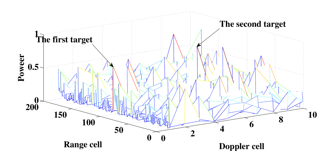

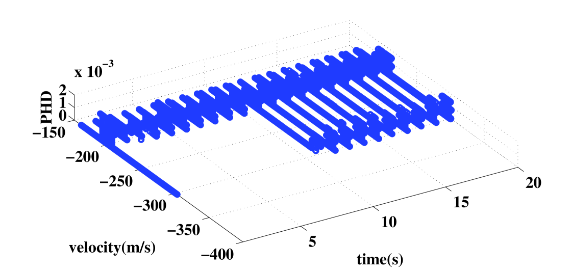
In the first example, the SNRs of both targets are 9 dB. The measurements are shown in Fig. 3. Tracking with the shrinkage-PHD filter, we plot the PHD of the position and velocity versus time in Fig. 4 and 5. It is shown that the PHD of targets can be integrated over time by simultaneous detection and tracking. Observe that both trajectories are automatically initiated and tracked. In step 3, the first target can be tracked stably. At step 11, just 1 s after target spawning, the second target is already initiated and tracked.
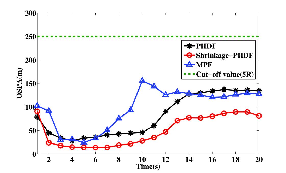
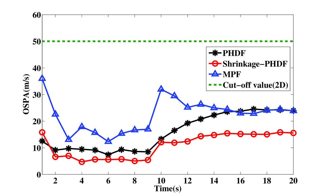
For the second example, we conducted simulations to compare the performance of the shrinkage-PHD filter (shrinkage-PHDF) the PHD filter (PHDF) Ref16 , and the classical multitarget particle filtering method (MPF) Ref8 in tracking accurately and consistently, and 50 Monte Carlo runs for the same scenario as used in the first example were performed. The states of targets are estimated by expectation-maximization (EM) algorithm. In addition, the maximum possible number of targets is limited and known for MPF, but unlimited and unknown for the PHD filter and the shrinkage-PHDF.
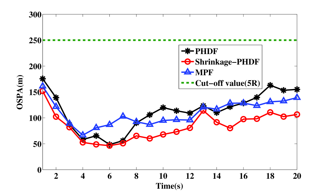
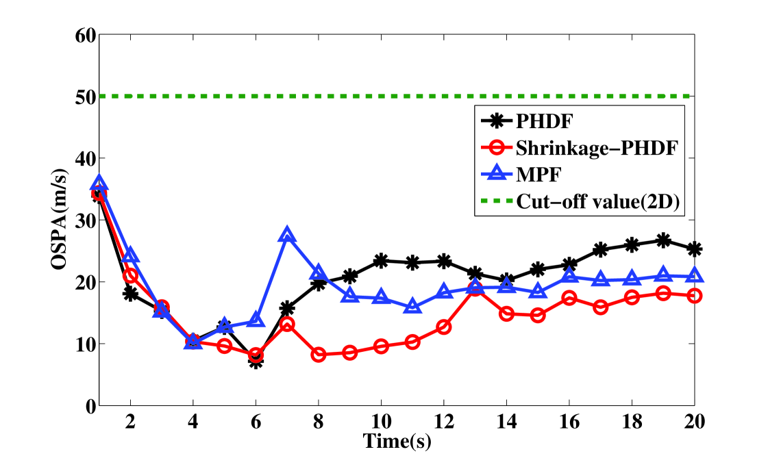
To measure the estimation quantitatively, the estimation errors in terms of Monte Carlo averaged OSPA distance are shown in Figs. 6 and 7. For position estimation, the cut-off value c is five times the size of the range cell. For velocity estimation, the cut-off value c is two times the size of the velocity cell. It is shown that the shrinkage-PHDF estimates target position and velocity on all tracks with higher estimated precision than the MPF, because MPF requires a modeling setup to accommodate varying numbers of targets, which is very difficult to accomplish in reality.It also shows that the performance of shrinkage-PHDF is better than PHDF, which is discussed further below.
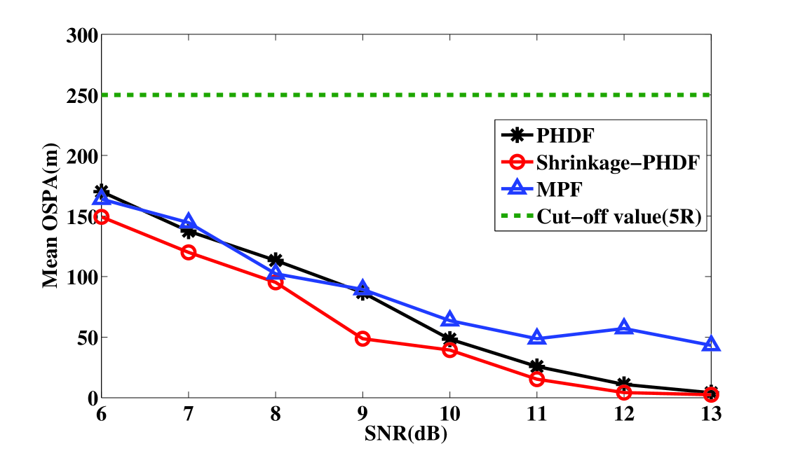
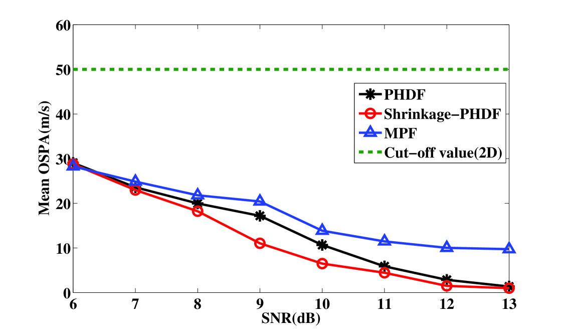
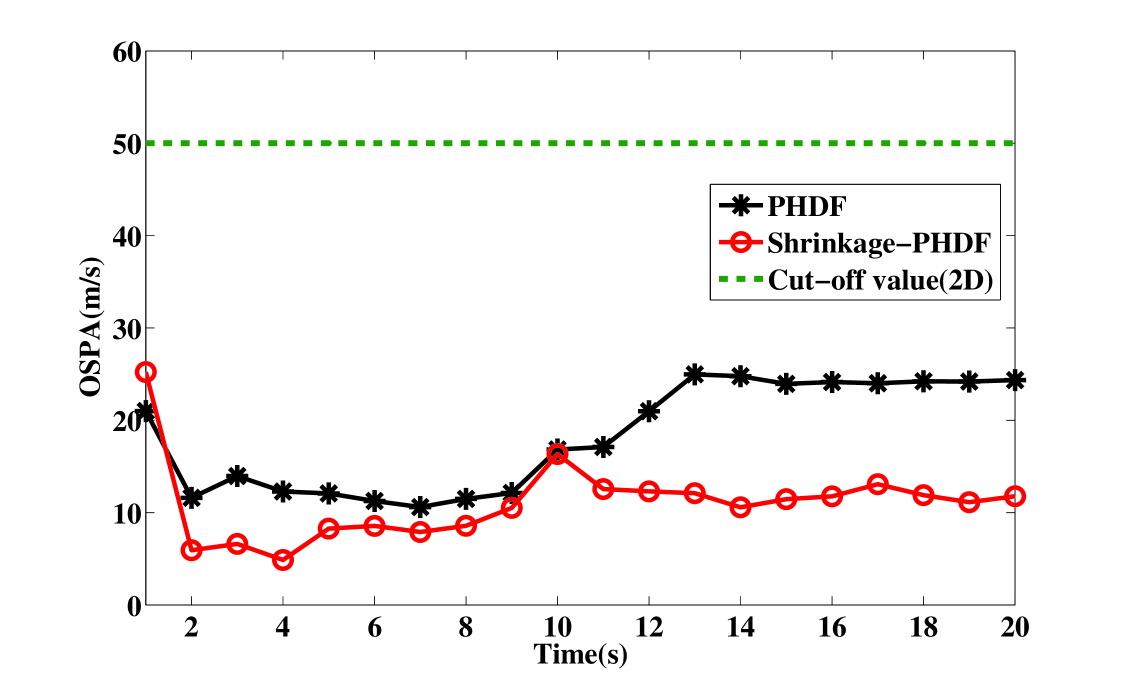
To compare the shrinkage-PHDF and the PHDF clearly, Figs. 8 and 9 show the comparison of the mean OSPA for varying SNRs. The SNR of the targets is set to known values between 6 and 13 dB. When the value is between 6 and 11 dB, the shrinkage-PHDF performs significantly better than the PHDF. When the value is large than 11 dB, they perform similarly. This finding illustrates the limitation of ordinary the PHDF for TBD: the PHD cannot sufficiently approximate the multitarget posterior probability when the SNR is low. The superiority of the shrinkage-PHDF takes advantage of the shrinkage operation is indicated, especially for low SNR scenarios. It is clear that for multitarget TBD, the shrinkage-PHDF performs better than the PHDF and MPF, especially when the SNR is low.
6.3 Multiple targets with different SNRs
In this example, the targets with different SNRs (the first target is 8dB, the second target is 9dB and the last one is 10dB). At time step1, the first target appears as in the first example. At step 7,the second target spawns form the first one, and the velocity in the x-direction is -300m/s. The third target new-birth far from the previous two targets at the time step 13 with the intital target state . A comparison of the estimation errors of the position and the velocity of the three algorithms is shown in Fig. 10 and 11. In this scene, the targets vary not only the value of SNRs but also the average number of targets. Because the SNR of the first target is lower than which in section 6.2, the convergence velocity of the estimation first target is slower. After time step 7, comparing Figs. 6 and 10, Fig.7 and 11, the varying SNRs and the number of the targets did not significantly influence the performance of the PHDF and Shrinkage-PHDF. In this example, the performance of MPF is better than that in the first example. The reason is the intensity of the targets is the most important characteristic to differentiate different targets for MPF method. In this way, the SNRs of all targets should be known for MPF method.
6.4 Multiple targets with unknown SNRs
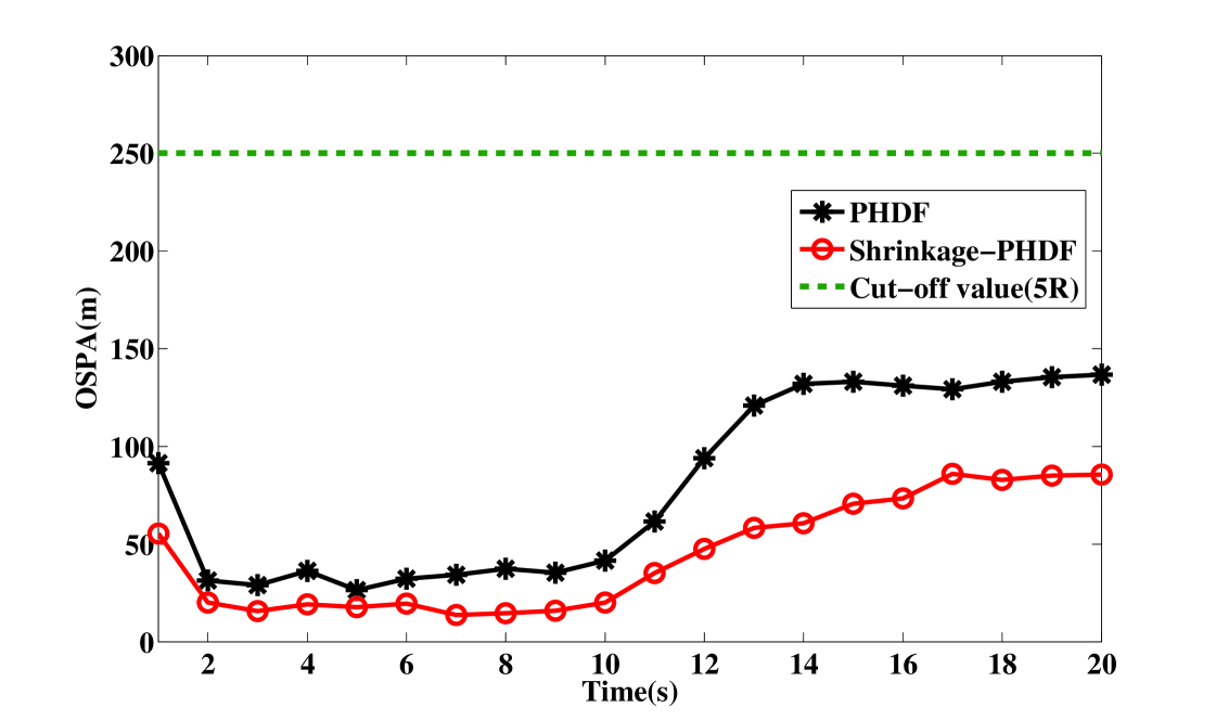
The PHD filter and the shrinkage-PHD filter are compared in Fig. 12 and 13. The sense is similar with that in the section 6.2, but the SNRs of the targets are unknown and the SNR of the second target changes from 9dB to 10dB. It is obvious that the performance of both algorithms is similar to what was presented in Figs. 6 and 7. After the 11th time step, the performance is even better than which in the section 6.2, because the value of the SNR of the second target is increased. Therefore, whether the SNRs of multiple targets are known has not significant influence on the performance of PHDF and Shrinkage-PHDF. In addition, MPF from Ref8 does not work when the value of the SNRs of the targets are unknown.
6.5 A comparison of computation resources
| Algorithm | Shrinkage-PHDF | PHDF | MPF |
| Computation(Second) | 28.66 | 28.12 | 84.20 |
Table 3 shows the computation resources needed for the PHDF, the shrinkage-PHDF and MPF. All simulations were run on a PC with an Intel (R) Core TM2 Duo CPU E4500 @ 2.20 GHz processor. The time listed is Monte Carlo-averaged, for a run in a scenario similar to that given in Section 6.2. The amount of calculation time required for the shrinkage-PHDF and the PHDF is much less than for MPF. The calculated amount time required for the shrinkage-PHDF is slightly greater than that required for the PHD filter.
7 Conclusion
In this paper, we used the RFS to model multitarget TBD measurements and to design an efficient Shrinkage-PHD filter for multitarget TBD. This filter accompanies with a shrinkage operation, and the optimal parameter for the shrinkage operation is obtained by an optimization procedure. Simulations show that the shrinkage-PHD filter takes very little time to detect new targets, and it is sensitive to the variation in the number of targets. Moreover, our algorithm can track targets with high accuracy by taking advantage of the shrinkage operation. In addition, there is no restriction on the maximum number of possible targets or known value of SNRs of targets. In a word, by the application of Shrinkage-PHD filter, multiple targets could be tracked well in low SNR environments.
In the future research, a challenge to be explored for the shrinkage-PHD filter will be determining how to model the measurement of extended targets in the framework of FISST. If this issue is resolved, it is believed that our new approach will be useful in future radar systems using the TBD technique.
References
- (1) B.Ristic, S.Arulampalam, and N.Gordon, Beyond the Kalman filter-particle filters for tracking applications pp.239-240, Artech House, Boston, MA, USA, (2004)
- (2) J. H. Zwaga, J. N. Driessen, and W. J. H. Meijer, Track-before-detect for surveillance radar: a recursive filter based approach, Proc. SPIE-Int. Soc. Opt. Eng, Vol 4728, pp. 103-115, (2002)
- (3) M. Hadzagic, H. Michalska, E. Lefebvre, Track-before detect methods in tracking low-observable targets: a survey, Sensors & Transducers Magazine, Special Issue 1, pp.374-380, (2005)
- (4) S. J. Davey, M. G. Rutten, and B. Cheung, A comparison of detection performance for several track-before-detect algorithms, EURASIP Journal on Advances in Signal Processing, Vol. 2008 , Issue 1, Article 41, (2008)
- (5) O. Nichtern, S. R. Rotman, Search radar detection and track with the Hough transform, EURASIP Journal on Advances in Signal Processing, Volume 2008, Article ID 146925, 19 pages, (2008)
- (6) L. A. Johnston and V. Krishnamurthy, Parameter adjustment for a dynamic programming track-before-detect-based target detection algorithm, IEEE Transactions on Aerospace and Electronic Systems, Vol 38, pp. 228-242, (2002)
- (7) S. M. Tonbsen and Y. Bar-Shalom, Maximum likelihood track-before-detect with fluctuating target amplitude, IEEE Transactions on Aerospace and Electronic Systems, Vol 34, pp. 796-808, (1998)
- (8) Y. Boers and J. N. Driessen, Multitarget particle filter track before detect application, IEE Proceedings on Radar, Sonar and Navigation, Vol 151, No. 6, pp. 351-357, (2004)
- (9) –, Particle filter track-before-detect application using inequality constraints, IEEE transactions on Aerospace and Electronic Systems, Vol 41, No. 4, pp. 1481-1487, (2005).
- (10) K. Punithakumar, T. Kirubarajan and A. Sinha, A sequential Monte Carlo probability hypothesis density algorithm for multitarget track-before-detect, Proc. of SPIE Vol 5913, 59131S, (2005)
- (11) L. D. Stone, C. A. Barlow, and T. L. Corwin, Bayesian Multiple Target Tracking. Boston: Artech House, (1999)
- (12) B.-N. Vo, S. Singh and A. Doucet, Sequential Monte Carlo implementation of the PHD filter for multitarget tracking, Proc. 6th Int. Conf. Information Fusion, Vol 2, pp. 792-799, (2003)
- (13) R. Mahler, Multitarget Bayes filtering via first-order multitarget moments, IEEE Transactions on Aerospace and Electronic Systems, Vol 39, No. 4, pp. 1152-1178, (2003)
- (14) B.-N. Vo, and W.-K Ma, The gaussian mixture probability hypothesis density filter, IEEE Transactions on Signal Processing, Vol 54, No. 11, pp. 4091-4104, (2006)
- (15) B.-N. Vo, B.-T Vo, N.-T Pham, and D. Suter, Joint detection and estimation of multiple objects from image observations, IEEE Transaction on Signal Processing, Vol 58, No. 10, pp. 5129-5241, ( 2010)
- (16) H. Tong, H. Zhang, H. Meng, and X. Wang, Multitarget Tracking Before Detection via Probability Hypothesis Density Filter, in Proc. The International Conference on Electrical and Control Engineering, Wuhan, China, June. 26-June. 28, pp. 1332-1335, (2010).
- (17) O. Erdinc, P.Willett, and Y. Bar-Shalom, Probability hypothesis density filter for multitarget multisensor tracking, Proc. 8th Int. Conf. Information Fusion, Philadelphia, PA, USA, July 25-28, (2005)
- (18) R. Mahler, PHD filters of higher order in target number, IEEE Trans. Aerospace & Electronic Systems, Vol 43, No. 4, pp. 1523-1543, (2007)
- (19) N. Weyrich, G. T. Warhola, Wavelet shrinkage and generalized cross validation for image denoising, IEEE Transactions on Image Processing, Vol 7, No. 1, pp. 82-90, (1998)
- (20) D. Clark, B. Ristic, B.-N. Vo, and B.-T Vo, Bayesian multi-object filtering with amplitude feature likelihood for unknown object SNR, IEEE Transaction on Signal Processing, Vol 58, No. 1, pp. 26-36, (2010)
- (21) R. Mahler, PHD filters for nonstandard targets, I.: extended targets, Proc. 12th Int. Conf. Information Fusion, Seattle, WA, USA, July 6-9, (2009)
- (22) F. Lian, C.-Z. Han, W.-F. Liu, X.-X. Yan, H.-Y. Zhou, Sequential Monte Carlo implementation and state extraction of the group probability hypothesis density filter for partly unresolvable group targets-tracking problem, IET Radar, Sonar and Navigation, Vol 4, No. 5, pp. 685-702, (2010)
- (23) C.M. Bishop, Pattern recognition and machine learning. Springer,(2006)
- (24) D.Clark, B.Ristic, B.-N. Vo, B.-T. Vo, Bayesian multi-object filtering with amplitude feature likelihood for unknown object SNR. IEEE Transactions on Signal Processing, Vol 58, N0. 1,pp.26-37,(2010)