This paper was converted on www.awesomepapers.org from LaTeX by an anonymous user.
Want to know more? Visit the Converter page.

A Simple and Efficient Estimation of the Average Treatment Effect in the Presence of Unmeasured Confounders

Chunrong Ai E-mail: chunrong.ai@warrington.ufl.edu Lukang Huang E-mail: huanglukang@ruc.edu.cn Zheng Zhang E-mail: zhengzhang@ruc.edu.cn
Abstract

Wang and Tchetgen Tchetgen (2017) studied identification and estimation of the average treatment effect when some confounders are unmeasured. Under their identification condition, they showed that the semiparametric efficient influence function depends on five unknown functionals. They proposed to parameterize all functionals and estimate the average treatment effect from the efficient influence function by replacing the unknown functionals with estimated functionals. They established that their estimator is consistent when certain functionals are correctly specified and attains the semiparametric efficiency bound when all functionals are correctly specified. In applications, it is likely that those functionals could all be misspecified. Consequently their estimator could be inconsistent or consistent but not efficient. This paper presents an alternative estimator that does not require parameterization of any of the functionals. We establish that the proposed estimator is always consistent and always attains the semiparametric efficiency bound. A simple and intuitive estimator of the asymptotic variance is presented, and a small scale simulation study reveals that the proposed estimation outperforms the existing alternatives in finite samples.

Keywords: Average treatment effect; Unmeasured confounders; Semiparametric efficiency; Endogeneity.

1 Introduction

A common approach to account for individual heterogeneity in the treatment effect literature on observational data is to assume that there exist confounders, and conditional on these confounders, there is no systematic selection into the treatment (i.e., the so-called Unconfounded Treatment Assignment condition suggested in Rosenbaum and Rubin (1983, 1984)). Under this assumption, several procedures for estimating the average treament effect (hereafter ATE) have been proposed, including the weighting procedure (Rosenbaum (1987), Hirano, Imbens, and Ridder (2003), Tan (2010), Imai and Ratkovic (2014), Chan, Yam, and Zhang (2016), Yiu and Su (2018)); the matching procedure (Rosenbaum (2002), Rosenbaum et al. (2002), Dehejia and Wahba (1999)); and the regression procedure (Heckman, Ichimura, and Todd (1997), Heckman, Ichimura, and Todd (1998), Imbens, Newey, and Ridder (2006), Chen, Hong, and Tarozzi (2008)). For example survey, see Imbens and Wooldridge (2009) and Imbens and Rubin (2015). A critical requirement in this literature is that all confounders are observed and available to researchers. In applications, however, it is often the case that some confounders are either not observed or not availale. In this case, the average treatment effect is only partially identified even with the aid of some insrumental variables (see Imbens and Angrist (1994), Angrist, Imbens, and Rubin (1996), Abadie (2003), Abadie, Angrist, and Imbens (2002), Tan (2006), Cheng, Small, Tan, and Have (2009), Ogburn, Rotnitzky, and Robins (2015) for examples).

Recently Wang and Tchetgen Tchetgen (2017) suggested a noval identification condition of ATE when some confounders are not available. Under their condition, they showed that the semiparametric efficient influence function of ATE depends on five unknown functionals. They proposed to parameterize all five functionals, estimate those functionals with appropriate parametric approaches, plug the estimated functionals into the influence function, and then estimate the ATE from the estimated influence function. They established that their estimator is consistent if certain functionals are correctly parameterized and attains the semiparametric efficiency bound if all functionals are correctly specified. In applications, it is quite possible that some or all of the five functionals are misspecified and consequently their estimator could be inefficient or worse, inconsistent. This paper proposes an alternative, intuitive and easy to compute estimation that does not require parameterization of any of the five unknown functionals. We estbalish that under some sufficient conditions the proposed estimator is consistent, asymptotically normally distributed and attains the semiparametric efficiency bound. Moreover, the proposed procedure provides a natural and convenient estimate of the asymptotic variance.

The paper is organized as follows. Section 2 describes the basic framework. Section 3 describes the proposed estimation and derives the large sample properties of the proposed estimator. Section 4 presents a consistent variance estimator. Since the proposed procedure depends on smoothing parameters, Section 5 presents a data driven method for selecting the smoothing paprameters. Section 6 reports a small scale simulation study to evaluate the finite sample performance of the proposed estimator. Some concluding remarks are in Section 7. All technical proofs are relegated to the Appendix and the supplementary material.

2 Basic Framework

Let D{0,1}D\in\{0,1\} denote the binary treatment indicator, and let Y(1)Y(1) and Y(0)Y(0) denote the potential outcomes when an individual is assigned to the treatment and control group respectively. The parameter of interest is the population average treatment effect τ=𝔼[Y(1)Y(0)]\tau=\mathbb{E}[Y(1)-Y(0)]. Estimation of τ\tau is complicated by the presence of confounders and the fact that Y(1)Y(1) and Y(0)Y(0) cannot be observed simultaneously. To distinguish observed confounders from unobserved confounders, we shall use XX to denote the observed confounders and use UU to denote the unmeasured confounders. It is well established in the literature that, when all confounders are observed, the following Unconfounded Treatment Assignment condition is sufficient to identify τ\tau:

Assumption 2.1.

(Y(0),Y(1))(D,Z)|(X,U)(Y(0),Y(1))\perp(D,Z)|(X,U).

When UU is unmeasured, we have the classical omitted variable problem, causing the treament indicator DD to be endogenous. To tackle the endogeneity problem, instrumental variable is often the preferred choice. Let Z{0,1}Z\in\{0,1\} denote the variable satisfying the following classical instrumental variable conditions:

Assumption 2.2 (Exclusion restriction).

z,d\forall z,d, Y(z,d)=Y(d)Y(z,d)=Y(d), where Y(z,d)Y(z,d) is the response that would be observed if a unit were exposed to dd and the instrument had taken value zz to be well defined.

Assumption 2.3 (Independence).

ZU|XZ\perp U|X.

Assumption 2.4 (IV relavance).

Z⟂̸D|XZ\not\perp D|X.

Wang and Tchetgen Tchetgen (2017) showed that Asssumptions 2.1- 2.4 alone do not identify τ\tau, but if in addition one of the following conditions holds:

  1. 1.

    there is no additive UU-ZZ interaction in 𝔼[D|Z,X,U]\mathbb{E}[D|Z,X,U]:

    𝔼[D|Z=1,X,U]𝔼[D|Z=0,X,U]=𝔼[D|Z=1,X]𝔼[D|Z=0,X].\mathbb{E}[D|Z=1,X,U]-\mathbb{E}[D|Z=0,X,U]=\mathbb{E}[D|Z=1,X]-\mathbb{E}[D|Z=0,X]\ .
  2. 2.

    there is no additive UU-dd interaction in 𝔼[Y(d)|X,U]\mathbb{E}[Y(d)|X,U]:

    𝔼[Y(1)Y(0)|X,U]=𝔼[Y(1)Y(0)|X],\mathbb{E}[Y(1)-Y(0)|X,U]=\mathbb{E}[Y(1)-Y(0)|X]\ ,

then ATE is identified and can be expressed as

τ=𝔼[δ(X)]=𝔼[δY(X)δD(X)],\displaystyle\tau=\mathbb{E}[\delta(X)]=\mathbb{E}\left[\frac{\delta^{Y}(X)}{\delta^{D}(X)}\right]\ , (2.1)

where

δY(X)=𝔼[Y|Z=1,X]𝔼[Y|Z=0,X],\displaystyle\delta^{Y}(X)=\mathbb{E}[Y|Z=1,X]-\mathbb{E}[Y|Z=0,X]\ ,
δD(X)=𝔼[D|Z=1,X]𝔼[D|Z=0,X],\displaystyle\delta^{D}(X)=\mathbb{E}[D|Z=1,X]-\mathbb{E}[D|Z=0,X]\ ,
δ(X)=δY(X)/δD(X).\displaystyle\delta(X)=\delta^{Y}(X)/\delta^{D}(X)\ .

Furthermore, Wang and Tchetgen Tchetgen (2017) derived the efficient influence function for τ\tau:

φeff(D,Z,X,Y)=2Z1fZ|X(Z|X)1δD(X){YDδ(X)𝔼[Y|Z=0,X]+𝔼[D|Z=0,X]δ(X)}+δ(X)τ,\varphi_{eff}(D,Z,X,Y)=\frac{2Z-1}{f_{Z|X}(Z|X)}\frac{1}{\delta^{D}(X)}\bigg{\{}Y-D\delta(X)-\mathbb{E}[Y|Z=0,X]+\mathbb{E}[D|Z=0,X]\delta(X)\bigg{\}}+\delta(X)-\tau\ ,

where fZ|X(Z|X)f_{Z|X}(Z|X) is the conditional probability mass function of ZZ given XX. Clearly, the efficient influence function depends on five unknown functionals: δ(X)\delta(X), δD(X)\delta^{D}(X), fZ|Xf_{Z|X}, p0Y(X)=𝔼[Y|Z=0,X]p_{0}^{Y}(X)=\mathbb{E}[Y|Z=0,X] and p0D(X)=𝔼[D|Z=0,X]p_{0}^{D}(X)=\mathbb{E}[D|Z=0,X]. They proposed to parameterize all five functionals, estimate the functionals with appropriate parametric approaches, and plug the estimated functionals into the efficient influence function to estimate τ\tau. They established that their estimator of τ\tau is consistent and asymptotically normally distributed if

  • either δ(X)\delta(X), δD(X)\delta^{D}(X), p0Y(X)=𝔼[Y|Z=0,X]p_{0}^{Y}(X)=\mathbb{E}[Y|Z=0,X] and p0D(X)=𝔼[D|Z=0,X]p_{0}^{D}(X)=\mathbb{E}[D|Z=0,X] are correctly specified

  • or δD(X)\delta^{D}(X) and fZ|Xf_{Z|X} are correctly specified

  • or δ(X)\delta(X) and fZ|Xf_{Z|X} are correctly specified,

and their estimator attains the semiparametric efficiency bound only when all five functionals are correctly specified. The main goal of this paper is to present an alternative, intuitive and easy approach to compute estimator that does not require parameterization of any of the functionals and is always consistent and asymptotically normal and attains the semiparametric efficiency bound.

3 Point Estimation

To motivate our estimation procedure, we rewrite the treatment effect coefficient. Applying the tower law of conditional expectation, we obtain:

τ=\displaystyle\tau= 𝔼[δY(X)δD(X)]=𝔼[𝔼[Y|Z=1,X]δD(X)𝔼[Y|Z=0,X]δD(X)]\displaystyle\mathbb{E}\left[\frac{\delta^{Y}(X)}{\delta^{D}(X)}\right]=\mathbb{E}\left[\frac{\mathbb{E}[Y|Z=1,X]}{\delta^{D}(X)}-\frac{\mathbb{E}[Y|Z=0,X]}{\delta^{D}(X)}\right]
=\displaystyle= 𝔼[ZfZ|X(1|X)𝔼[Y|Z=1,X]δD(X)1ZfZ|X(0|X)𝔼[Y|Z=0,X]δD(X)]\displaystyle\mathbb{E}\left[\frac{Z}{f_{Z|X}(1|X)}\cdot\frac{\mathbb{E}[Y|Z=1,X]}{\delta^{D}(X)}-\frac{1-Z}{f_{Z|X}(0|X)}\cdot\frac{\mathbb{E}[Y|Z=0,X]}{\delta^{D}(X)}\right]
=\displaystyle= 𝔼[ZfZ|X(1|X)𝔼[Y|Z,X]δD(X)1ZfZ|X(0|X)𝔼[Y|Z,X]δD(X)]\displaystyle\mathbb{E}\left[\frac{Z}{f_{Z|X}(1|X)}\cdot\frac{\mathbb{E}[Y|Z,X]}{\delta^{D}(X)}-\frac{1-Z}{f_{Z|X}(0|X)}\cdot\frac{\mathbb{E}[Y|Z,X]}{\delta^{D}(X)}\right]
=\displaystyle= 𝔼[{2Z1fZ|X(Z|X)}YδD(X)].\displaystyle\mathbb{E}\left[\left\{\frac{2Z-1}{f_{Z|X}(Z|X)}\right\}\frac{Y}{\delta^{D}(X)}\right]\ . (3.1)

The above expression suggests a natural and intuitive plugin estimation, with fZ|X(Z|X)f_{Z|X}(Z|X) and δD(X)\delta^{D}(X) replaced by some consistent estimates. There are many approaches to estimate these functionals including parametric and nonparametric approaches, but as noted by Hirano, Imbens, and Ridder (2003), not all estimates can lead to efficient estimation of τ\tau. In this paper, we present an intuitive and easy way to compute estimates of functionals that ensure efficiency of the plugin estimation of τ\tau. To illustrate our procedure, we notice that the following conditions hold for any integrable functions u1(X)u_{1}(X) and u2(X)u_{2}(X):

𝔼[ZfZ|X(1|X)u1(X)]=𝔼[u1(X)]=𝔼[1ZfZ|X(0|X)u1(X)],\displaystyle\mathbb{E}\left[\frac{Z}{f_{Z|X}(1|X)}u_{1}(X)\right]=\mathbb{E}[u_{1}(X)]\ =\mathbb{E}\left[\frac{1-Z}{f_{Z|X}(0|X)}u_{1}(X)\right], (3.2)
𝔼[D{2Z1fZ|X(Z|X)}u2(X)]=𝔼[δD(X)u2(X)],\displaystyle\mathbb{E}\left[D\left\{\frac{2Z-1}{f_{Z|X}(Z|X)}\right\}u_{2}(X)\right]=\mathbb{E}\left[\delta^{D}(X)u_{2}(X)\right]\ , (3.3)

and (3.2) and (3.3) uniquely determine fZ|X(Z|X)f_{Z|X}(Z|X) and δD(X)\delta^{D}(X). These conditions impose restrictions on the unknown functionals and they must be taken into account when estimating those functionals. One difficulty with these conditions is that they must be imposed in an infinite dimmensional functional space. To overcome this difficulty, we propose to impose the conditions on a smaller sieve space. Specifically, let uK(X)=(uK,1(X),,uK,K(X))u_{K}(X)=(u_{K,1}(X),\ldots,u_{K,K}(X))^{\top} denote a known basis functions that can approximate any suitable function u(X)u(X) arbitrarily well (see Chen (2007) or Appendix A.1 for further dicussion). Conditions (3.2) and (3.3) imply for any integers K1K_{1} and K2K_{2}:

𝔼[ZfZ|X(1|X)uK1(X)]=𝔼[uK1(X)]=𝔼[1ZfZ|X(0|X)uK1(X)]\mathbb{E}\left[\frac{Z}{f_{Z|X}(1|X)}u_{K_{1}}(X)\right]=\mathbb{E}[u_{K_{1}}(X)]=\mathbb{E}\left[\frac{1-Z}{f_{Z|X}(0|X)}u_{K_{1}}(X)\right]\ (3.4)

and

𝔼[D{ZfZ|X(1|X)1ZfZ|X(0|X)}uK2(X)]=𝔼[δD(X)uK2(X)].\mathbb{E}\left[D\left\{\frac{Z}{f_{Z|X}(1|X)}-\frac{1-Z}{f_{Z|X}(0|X)}\right\}u_{K_{2}}(X)\right]=\mathbb{E}[\delta^{D}(X)u_{K_{2}}(X)].\ (3.5)

We shall construct estimates of the functionals by imposing the above conditions. To ensure consistency, we shall allow K1K_{1} and K2K_{2} to increase with sample size at appropriate rates.

3.1 Estimation of fZ|X(Z|X)1f_{Z|X}(Z|X)^{-1}

Consider estimation of fZ|X(Z|X)1f_{Z|X}(Z|X)^{-1}. An obvious approach is to solve {wi,i=1,2,,N}\left\{w_{i},i=1,2,...,N\right\} from the sample analogue of (3.4):

1Ni=1NZiwiuK1(Xi)\displaystyle\frac{1}{N}\sum_{i=1}^{N}Z_{i}w_{i}u_{K_{1}}({X}_{i}) =\displaystyle= 1Ni=1NuK1(Xi);\displaystyle\frac{1}{N}\sum_{i=1}^{N}u_{K_{1}}({X}_{i}); (3.6)
1Ni=1N(1Zi)wiuK1(Xi)\displaystyle\frac{1}{N}\sum_{i=1}^{N}(1-Z_{i})w_{i}u_{K_{1}}({X}_{i}) =\displaystyle= 1Ni=1NuK1(Xi).\displaystyle\frac{1}{N}\sum_{i=1}^{N}u_{K_{1}}({X}_{i}). (3.7)

But there are many solutions and all solutions are consistent estimates of fZ|X(Z|X)1f_{Z|X}(Z|X)^{-1}. The question is which solution is the best estimate of fZ|X(Z|X)1f_{Z|X}(Z|X)^{-1} in the sense of ensuring efficient estimation of τ\tau. Let ρ(v)\rho(v) denote a strictly increasing and concave function and let ρ(v)\rho^{\prime}(v) denote its first derivative. Denote

p^(Xi)1Nρ(λ^K1uK1(Xi)),\hat{p}(X_{i})\triangleq\frac{1}{N}\rho^{\prime}(\hat{\lambda}_{K_{1}}^{\top}u_{K_{1}}(X_{i}))\ ,

with λ^K1K\hat{\lambda}_{K_{1}}\in\mathbb{R}^{K} maximizing the following objective function

G^(λ)1Ni=1NZiρ(λuK1(Xi))1Ni=1NλuK1(Xi).\hat{G}(\lambda)\triangleq\frac{1}{N}\sum_{i=1}^{N}Z_{i}\rho(\lambda^{\top}u_{K_{1}}(X_{i}))-\frac{1}{N}\sum_{i=1}^{N}\lambda^{\top}u_{K_{1}}(X_{i})\ . (3.8)

It is easy to show that Np^(X)N\hat{p}(X) satisfies (3.6). Moreover, Np^(X)N\hat{p}(X) can be interpreted as a generalized empirical likelihood estimator of fZ|X(1|X)1f_{Z|X}(1|X)^{-1} (see Appendix A.2) and hence is the best estimate. The fact that G^(λ)\hat{G}(\lambda) is globally concave implies that its maximand is easy to compute.

Applying the same idea to (3.7), we have

q^(Xi)1Nρ(β^K1uK1(Xi)),\hat{q}(X_{i})\triangleq\frac{1}{N}\rho^{\prime}(\hat{\beta}_{K_{1}}^{\top}u_{K_{1}}({X}_{i}))\ ,

with β^K1K1\hat{\beta}_{K_{1}}\in\mathbb{R}^{K_{1}} maximizing the following globally concave objective function

H^(β)1Ni=1N(1Zi)ρ(βuK1(Xi))1Ni=1NβuK1(Xi).\hat{H}(\beta)\triangleq\frac{1}{N}\sum_{i=1}^{N}(1-Z_{i})\rho(\beta^{\top}u_{K_{1}}(X_{i}))-\frac{1}{N}\sum_{i=1}^{N}\beta^{\top}u_{K_{1}}(X_{i}). (3.9)

Again, Nq^(X)N\hat{q}(X) satisfies (3.7) and can be interpreted as a generalized empirical likelihood estimatior of fZ|X(0|X)1f_{Z|X}(0|X)^{-1}.

The ρ(v)\rho(v) function can be any increasing and strictly concave function. Some examples include ρ(v)=exp(v)\rho(v)=-\exp(-v) for the exponential tilting (Kitamura and Stutzer, 1997, Imbens, Spady, and Johnson, 1998), ρ(v)=log(1+v)\rho(v)=\log(1+v) for the empirical likelihood (Owen, 1988, Qin and Lawless, 1994), ρ(v)=(1v)2/2\rho(v)=-(1-v)^{2}/2 for the continuous updating of the generalized method of moments (Hansen, 1982, Hansen, Heaton, and Yaron, 1996) and ρ(v)=vexp(v)\rho(v)=v-\exp(-v) for the inverse logistic.

3.2 Estimation of δD(X)\delta^{D}(X) and τ\tau

Having estimated fZ|X(Z|X)1f_{Z|X}(Z|X)^{-1}, we now apply the same principle to estimate δD(X)\delta_{D}(X). But there is one difference. Here δD(X)[1,1]\delta_{D}(X)\in[-1,1] and the ρ(v)\rho(v) function is not suitable. We shall use the following strictly convex function

f(x)=log(ex+ex)f(x)=\log(e^{x}+e^{-x})

whose derivative is the tanh function f(x)=exexex+exf^{\prime}(x)=\frac{e^{x}-e^{-x}}{e^{x}+e^{-x}} with range [1,1][-1,1]. We estimate δD(X)\delta^{D}(X) by

δ^D(X)=f(γ^K2uK2(X)),\hat{\delta}^{D}(X)=f^{\prime}(\hat{\gamma}_{K_{2}}^{\top}u_{K_{2}}(X)),

with γ^K2K2\hat{\gamma}_{K_{2}}\in\mathbb{R}^{K_{2}} maximizing the following globally concave function

F^(γ)=1Ni=1NDi{ZiNp^(Xi)(1Zi)Nq^(Xi)}γuK2(Xi)1Ni=1Nf(γuK2(Xi)).\hat{F}({\gamma})=\frac{1}{N}\sum_{i=1}^{N}D_{i}\{Z_{i}N\hat{p}(X_{i})-(1-Z_{i})N\hat{q}(X_{i})\}\cdot\gamma^{\top}u_{K_{2}}(X_{i})-\frac{1}{N}\sum_{i=1}^{N}f({\gamma}^{\top}u_{K_{2}}(X_{i})).

Again, δ^D(X)\hat{\delta}^{D}(X) can be interpreted as a generalized empirial likelihood estimator and hence is the best estimate.

Finally, the plugin estimator of τ\tau is given by

τ^=i=1N{Zip^(Xi)(1Zi)q^(Xi)}Yi/δ^D(Xi).\widehat{\tau}=\sum_{i=1}^{N}\left\{Z_{i}\hat{p}(X_{i})-(1-Z_{i})\hat{q}(X_{i})\right\}Y_{i}/\hat{\delta}^{D}(X_{i}).

3.3 Large Sample Properties

To establish the large sample properties of τ^\widehat{\tau}, we shall impose the following assumptions:

Assumption 3.1.

𝔼[1δD(X)2]<\mathbb{E}\left[\frac{1}{\delta^{D}(X)^{2}}\right]<\infty and 𝔼[Y2δD(X)4]<\mathbb{E}\left[\frac{Y^{2}}{\delta^{D}(X)^{4}}\right]<\infty.

Assumption 3.2.

The support 𝒳\mathcal{X} of rr-dimensional covariate XX is a Cartesian product of rr compact intervals.

Assumption 3.3.

We assume that there exist three positive constants >η1>η2>1>η3>0\infty>\eta_{1}>\eta_{2}>1>\eta_{3}>0 such that

η2fZ|X1(z|x)η1andη3δD(x)η3,(z,x){0,1}×𝒳.\eta_{2}\leq f^{-1}_{Z|X}(z|x)\leq\eta_{1}\ \ \text{and}\ \ -\eta_{3}\leq\delta^{D}(x)\leq\eta_{3}\ ,\quad\forall(z,x)\in\{0,1\}\times\mathcal{X}\ .
Assumption 3.4.

There are λK\lambda_{K}, βK\beta_{K}, γK\gamma_{K}, ψ1K\psi_{1K}, ψ0K\psi_{0K}, ϕ1K\phi_{1K} and ϕ0K\phi_{0K} in K\mathbb{R}^{K} and α>0\alpha>0 such that

supx𝒳|(ρ)1(1fZ|X(1|x))λKuK(x)|=O(Kα),supx𝒳|(ρ)1(1fZ|X(0|x))βKuK(x)|=O(Kα),\displaystyle\sup_{x\in\mathcal{X}}\left|(\rho^{\prime})^{-1}\left(\frac{1}{f_{Z|X}(1|x)}\right)-\lambda_{K}^{\top}u_{K}(x)\right|=O(K^{-\alpha})\ ,\ \sup_{x\in\mathcal{X}}\left|(\rho^{\prime})^{-1}\left(\frac{1}{f_{Z|X}(0|x)}\right)-\beta_{K}^{\top}u_{K}(x)\right|=O(K^{-\alpha})\ ,
supx𝒳|(f)1(δD(x))γKuK(x)|=O(Kα),\displaystyle\sup_{x\in\mathcal{X}}\left|(f^{\prime})^{-1}\left(\delta^{D}(x)\right)-\gamma_{K}^{\top}u_{K}(x)\right|=O(K^{-\alpha})\ ,
supx𝒳|p1Y(x)δD(x)ψ1KuK(x)|=O(Kα),supx𝒳|p0Y(x)δD(x)ψ0KuK(x)|=O(Kα),\displaystyle\sup_{x\in\mathcal{X}}\left|\frac{p_{1}^{Y}(x)}{\delta^{D}(x)}-\psi_{1K}^{\top}u_{K}(x)\right|=O(K^{-\alpha})\ ,\ \sup_{x\in\mathcal{X}}\left|\frac{p_{0}^{Y}(x)}{\delta^{D}(x)}-\psi_{0K}^{\top}u_{K}(x)\right|=O(K^{-\alpha})\ ,
supx𝒳|p1Y(x)δD(x)2ϕ1KuK(x)|=O(Kα),supx𝒳|p0Y(x)δD(x)2ϕ0KuK(x)|=O(Kα),\displaystyle\sup_{x\in\mathcal{X}}\left|\frac{p_{1}^{Y}(x)}{\delta^{D}(x)^{2}}-\phi_{1K}^{\top}u_{K}(x)\right|=O(K^{-\alpha})\ ,\ \sup_{x\in\mathcal{X}}\left|\frac{p_{0}^{Y}(x)}{\delta^{D}(x)^{2}}-\phi_{0K}^{\top}u_{K}(x)\right|=O(K^{-\alpha})\ ,

as KK\to\infty, where pzY(x)=𝔼[Y|Z=z,X=x]p_{z}^{Y}(x)=\mathbb{E}[Y|Z=z,X=x] for z{0,1}z\in\{0,1\}.

Assumption 3.5.

K1K2KK_{1}\asymp K_{2}\asymp K\in\mathbb{N}, ζ(K)4K3/N0\zeta(K)^{4}K^{3}/N\to 0 and NKα0\sqrt{N}K^{-\alpha}\to 0, where ζ(K)=supx𝒳uK(x)\zeta(K)=\sup_{x\in\mathcal{X}}\|u_{K}(x)\| and \|\cdot\| is the usual Frobenius norm defined by A=tr(AA)\|A\|=\sqrt{\text{tr}(AA^{\top})} for any matrix AA.

Assumption 3.6.

ρ\rho is a strictly concave function defined on \mathbb{R}, i.e. ρ′′(γ)<0,γ\rho^{\prime\prime}(\gamma)<0,~\forall\gamma\in\mathbb{R}, and the range of ρ\rho^{\prime} contains [η2,η1][\eta_{2},\eta_{1}].

Assumption 3.1 ensures the asymptotic variance to be bounded. Assumption 3.2 restricts the covariates to be bounded. This condition, though restrictive, is commonly imposed in the nonparametric regression literature. Assumption 3.3 requires the probability function to be bounded away from 0 and 1. Condition of this sort is familiar in the literature. Assumption 3.4 is needed to control for the approximation bias, and they are commonly imposed in the nonparametric literature. Assumption 3.5 imposes restrictions on the smoothing parameter so that the proposed estimator of ATE is root-N consistent. This condition, however, is practically unhelpful. We shall present a data driven approach to determine K1K_{1} and K2K_{2}. Assumption 3.6 is a mild restriction on ρ\rho and is satisfied by all important special cases considered in the literature.

Under the above assumptions, the following theorem establishes the consistency, asymptotic normality and the semiparmetric efficiency of τ^\hat{\tau}.

Theorem 3.7.

Suppose that the average treatment effects is identified in (2.1), under Assumptions 3.1-3.6, we have

  1. 1.

    τ^𝑝τ\hat{\tau}\xrightarrow{p}\tau;

  2. 2.

    N(τ^τ)𝑑N(0,Veff)\sqrt{N}(\hat{\tau}-\tau)\xrightarrow{d}N(0,V_{eff}),

where Veff=𝔼[φeff(D,Z,X,Y)2]V_{eff}=\mathbb{E}\left[\varphi_{eff}(D,Z,X,Y)^{2}\right] is the efficient variance bound developed in Wang and Tchetgen Tchetgen (2017).

Sketched proof can be found in Appendix A.4 and detailed proofs are provided in the supplementary material.

4 Variance Estimation

To conduct the statistical inference on τ\tau, we need a consistent estimator of the asymptotic variance of τ^\widehat{\tau}. Note that the asymptotic varance of τ^\widehat{\tau},

𝔼[(2Z1fZ|X(Z|X)1δD(X){YDδ(X)𝔼[Y|Z=0,X]+𝔼[D|Z=0,X]δ(X)}+δ(X)τ)2],\mathbb{E}\left[\left(\frac{2Z-1}{f_{Z|X}(Z|X)}\frac{1}{\delta^{D}(X)}\bigg{\{}Y-D\delta(X)-\mathbb{E}[Y|Z=0,X]+\mathbb{E}[D|Z=0,X]\delta(X)\bigg{\}}+\delta(X)-\tau\right)^{2}\right]\ ,

depends on five unknown functionals. Direct estimation of the variance requires replacing the five unknown functionals with consistent estimates. In this section, we present an alternative estimation that does not require estimation of those functionals.

To illustrate the idea, we denote:

g1(Z,X;λ)Zρ(λuK1(X))uK1(X)uK1(X),\displaystyle g_{1}(Z,{X};\lambda)\triangleq Z\rho^{\prime}\left(\lambda^{\top}u_{K_{1}}({X})\right)u_{K_{1}}({X})-u_{K_{1}}({X})\ ,
g2(Z,X;β)(1Z)ρ(βuK1(X))uK1(X)uK1(X),\displaystyle g_{2}(Z,{X};\beta)\triangleq(1-Z)\rho^{\prime}\left(\beta^{\top}u_{K_{1}}({X})\right)u_{K_{1}}({X})-u_{K_{1}}({X})\ ,
g3(Z,D,X;λ,β,γ)D{Zρ(λuK1(X))(1Z)ρ(βuK1(X))}uK2(X)f(γuK2(X))uK2(X),\displaystyle g_{3}(Z,D,{X};\lambda,\beta,\gamma)\triangleq D\left\{Z\cdot\rho^{\prime}\left(\lambda^{\top}u_{K_{1}}(X)\right)-(1-Z)\cdot\rho^{\prime}\left(\beta^{\top}u_{K_{1}}(X)\right)\right\}u_{K_{2}}({X})-f^{\prime}\left(\gamma^{\top}u_{K_{2}}({X})\right)u_{K_{2}}({X})\ ,
g4(Z,D,X,Y;λ,β,γ,τ){Zρ(λuK1(X))(1Z)ρ(βuK1(X))}Y/f(γuK2(X))τ,\displaystyle g_{4}(Z,D,X,Y;\lambda,\beta,\gamma,\tau)\triangleq\left\{Z\cdot\rho^{\prime}\left(\lambda^{\top}u_{K_{1}}(X)\right)-(1-Z)\cdot\rho^{\prime}\left(\beta^{\top}u_{K_{1}}(X)\right)\right\}Y/f^{\prime}\left(\gamma^{\top}u_{K_{2}}(X)\right)-\tau\ ,

and

g(Z,D,X,Y;θ)(g1(Z,X;λ)g2(Z,X;β)g3(Z,D,X;λ,β,γ)g4(Z,D,X,Y;λ,β,γ,τ))g(Z,D,X,Y;\theta)\triangleq\left(\begin{array}[]{c}g_{1}(Z,{X};\lambda)\\ g_{2}(Z,{X};\beta)\\ g_{3}(Z,D,{X};\lambda,\beta,\gamma)\\ g_{4}(Z,D,X,Y;\lambda,\beta,\gamma,\tau)\end{array}\right)

with θ(λ,β,γ,τ)\theta\triangleq(\lambda,\beta,\gamma,\tau)^{\top}. Let θ^(λ^K1,β^K1,γ^K2,τ^)\hat{\theta}\triangleq(\hat{\lambda}_{K_{1}},\hat{\beta}_{K_{1}},\hat{\gamma}_{K_{2}},\hat{\tau})^{\top} and θ(λK1,βK1,γK2,τ){\theta}^{\ast}\triangleq({\lambda}_{K_{1}}^{\ast},{\beta}_{K_{1}}^{\ast},{\gamma}_{K_{2}}^{\ast},{\tau})^{\top}. Then θ^\hat{\theta} is the moment estimator solving the following moment condition:

1Ni=1Ng(Zi,Di,Xi,Yi;θ^)=0.\frac{1}{N}\sum_{i=1}^{N}g(Z_{i},D_{i},X_{i},Y_{i};\hat{\theta})=0. (4.1)

Applying Mean Value Theorem, we obtain

0=1Ni=1Ng(Zi,Di,Xi,Yi;θ)+1Ni=1Ng(Zi,Di,Xi,Yi;θ~)θ(θ^θ)0=\frac{1}{N}\sum_{i=1}^{N}g(Z_{i},D_{i},X_{i},Y_{i};\theta^{\ast})+\frac{1}{N}\sum_{i=1}^{N}\frac{\partial g(Z_{i},D_{i},X_{i},Y_{i};\tilde{\theta})}{\partial\theta}(\hat{\theta}-\theta^{\ast}) (4.2)

where θ~=(λ~K1,β~K1,γ~K2,τ~)\tilde{\theta}=(\tilde{\lambda}_{K_{1}},\tilde{\beta}_{K_{1}},\tilde{\gamma}_{K_{2}},\tilde{\tau})^{\top} lies on the line joining θ^\hat{\theta} and θ\theta^{\ast}. We show in the supplemental material that

1Ni=1Ng(Zi,Di,Xi,Yi;θ~)θ=𝔼[g(Z,D,X,Y;θ)θ]+op(1)\frac{1}{N}\sum_{i=1}^{N}\frac{\partial g(Z_{i},D_{i},X_{i},Y_{i};\tilde{\theta})}{\partial\theta}=\mathbb{E}\left[\frac{\partial g(Z,D,X,Y;\theta^{\ast})}{\partial\theta}\right]+o_{p}(1) (4.3)

Note that

τ^τ=𝐞2K1+K2+1(θ^θ),\displaystyle\hat{\tau}-\tau=\mathbf{e}_{2K_{1}+K_{2}+1}^{\top}(\hat{\theta}-\theta^{\ast})\ , (4.4)

where 𝐞2K1+K2+1\mathbf{e}_{2K_{1}+K_{2}+1} is a (2K1+K2+1)(2K_{1}+K_{2}+1)-dimensional column vector whose last element is 11 and other components are all of 0’s.

Combining (4.2), (4.3) and (4.4), we obtain

N(τ^τ)=𝐞2K1+K2+1{𝔼[g(Z,D,X,Y;θ)θ]+op(1)}11Ni=1Ng(Zi,Di,Xi,Yi;θ),\sqrt{N}(\hat{\tau}-\tau)=-\mathbf{e}_{2K_{1}+K_{2}+1}^{\top}\left\{\mathbb{E}\left[\frac{\partial g(Z,D,X,Y;\theta^{\ast})}{\partial\theta}\right]+o_{p}(1)\right\}^{-1}\frac{1}{\sqrt{N}}\sum_{i=1}^{N}g(Z_{i},D_{i},X_{i},Y_{i};\theta^{\ast})\ ,

which in turn implies

Veff=limNVar(N(τ^τ))=limN𝐞2K1+K2+1{LΩ(L1)}𝐞2K1+K2+1.V_{eff}=\lim_{N\rightarrow\infty}Var(\sqrt{N}(\hat{\tau}-\tau))=\lim_{N\rightarrow\infty}\mathbf{e}_{2K_{1}+K_{2}+1}^{\top}\left\{L\cdot\Omega\cdot(L^{-1})^{\top}\right\}\mathbf{e}_{2K_{1}+K_{2}+1}\ .

where

L=𝔼[g(Z,D,X,Y;θ)θ],\displaystyle L=\mathbb{E}\left[\frac{\partial g(Z,D,X,Y;\theta^{\ast})}{\partial\theta}\right]\ ,
Ω=𝔼[g(Z,D,X,Y;θ)g(Z,D,X,Y;θ)].\displaystyle\Omega=\mathbb{E}\left[g(Z,D,X,Y;\theta^{\ast})g(Z,D,X,Y;\theta^{\ast})^{\top}\right]\ .

Therefore, we can define the sandwich estimator for the efficient variance VeffV_{eff} by

V^=𝐞2K1+K2+1{L^1Ω^(L^1)}𝐞2K1+K2+1,\hat{V}=\mathbf{e}_{2K_{1}+K_{2}+1}^{\top}\left\{\hat{L}^{-1}\cdot\hat{\Omega}\cdot(\hat{L}^{-1})^{\top}\right\}\mathbf{e}_{2K_{1}+K_{2}+1}\ ,

where

L^=1Ni=1Ng(Zi,Di,Xi,Yi;θ^)θ;\displaystyle\hat{L}=\frac{1}{N}\sum_{i=1}^{N}\frac{\partial g(Z_{i},D_{i},X_{i},Y_{i};\hat{\theta})}{\partial\theta};
Ω^=1Ni=1Ng(Zi,Di,Xi,Yi;θ^)g(Zi,Di,Xi,Yi;θ^).\displaystyle\hat{\Omega}=\frac{1}{N}\sum_{i=1}^{N}g(Z_{i},D_{i},X_{i},Y_{i};\hat{\theta})g(Z_{i},D_{i},X_{i},Y_{i};\hat{\theta})^{\top}.
Theorem 4.1.

Under Assumptions 3.1-3.6, V^\hat{V} is a consistent estimator for the asymptotic variance VeffV_{eff}.

5 Selection of Tuning Parameters

The large sample properties of the proposed estimator permit a wide range of values of K1K_{1} and K2K_{2}. This presents a dilemma for applied researchers who have only one finite sample and would like to have some guidance on the selection of smoothing parameters. In this section, we present a data-driven approach to select K1K_{1} and K2K_{2}. Notice that fZ|X(1|X)1f_{Z|X}(1|X)^{-1}, fZ|X(0|X)1f_{Z|X}(0|X)^{-1} and δD(X)\delta^{D}(X) satisfy the following regression equations:

𝔼[ZfZ|X(1|X)1|X]=1,\displaystyle\mathbb{E}\left[Zf_{Z|X}(1|X)^{-1}\bigg{|}X\right]=1\ ,
𝔼[(1Z)fZ|X(0|X)1|X]=1,\displaystyle\mathbb{E}\left[(1-Z)f_{Z|X}(0|X)^{-1}\bigg{|}X\right]=1\ ,
𝔼[D{ZfZ|X(1|X)1(1Z)fZ|X(0|X)1}|X]=δD(X).\displaystyle\mathbb{E}\left[D\left\{Zf_{Z|X}(1|X)^{-1}-(1-Z)f_{Z|X}(0|X)^{-1}\right\}\bigg{|}X\right]=\delta^{D}(X)\ .

Since Np^(X)N\hat{p}(X), Nq^(X)N\hat{q}(X) and δ^D(X)\hat{\delta}^{D}(X) are consistent estimators of fZ|X(1|X)1f_{Z|X}(1|X)^{-1}, fZ|X(0|X)1f_{Z|X}(0|X)^{-1} and δD(X)\delta^{D}(X) respectively, the mean-squared-error (MSE) of the nuisance parameters (λ^K1,β^K1)(\hat{\lambda}_{K_{1}},\hat{\beta}_{K_{1}}) and γ^K2\hat{\gamma}_{K_{2}} are defined by

MSE1(K1)=\displaystyle MSE_{1}(K_{1})= i=1N{ZiNp^(Xi)1}2+i=1N{(1Zi)Nq^(Xi)1}2,\displaystyle\sum_{i=1}^{N}\left\{Z_{i}N\hat{p}(X_{i})-1\right\}^{2}+\sum_{i=1}^{N}\left\{(1-Z_{i})N\hat{q}(X_{i})-1\right\}^{2}\ ,
MSE2(K1,K2)=\displaystyle MSE_{2}(K_{1},K_{2})= i=1N{Di{ZiNp^(Xi)(1Zi)Nq^(Xi)}δ^D(Xi)}2.\displaystyle\sum_{i=1}^{N}\left\{D_{i}\left\{Z_{i}N\hat{p}(X_{i})-(1-Z_{i})N\hat{q}(X_{i})\right\}-\hat{\delta}^{D}(X_{i})\right\}^{2}\ .

The smoothing parameters K1K_{1} and K2K_{2} shall be chosen to minimize MSE1MSE_{1} and MSE2MSE_{2}. Specifically, denote the upper bounds of K1K_{1} and K2K_{2} by K¯1\bar{K}_{1} and K¯2\bar{K}_{2} (e.g. K¯1=K¯2=5\bar{K}_{1}=\bar{K}_{2}=5 in our simulation studies). The data-driven K1K_{1} and K2K_{2} are given by

K^1=argminK1{1,,K¯1}MSE1(K1),\displaystyle\hat{K}_{1}=\arg\min_{K_{1}\in\{1,...,\bar{K}_{1}\}}MSE_{1}(K_{1})\ ,
K^2=argminK2{1,,K¯2}MSE2(K^1,K2).\displaystyle\hat{K}_{2}=\arg\min_{K_{2}\in\{1,...,\bar{K}_{2}\}}MSE_{2}(\hat{K}_{1},K_{2})\ .

6 Simulation Studies

In this section, we conduct a small scale simulation study to evaluate the finite sample performance of the proposed estimator. To evaluate the performance of our estimator against the existing alternatives, particularly the estimators proposed by Wang and Tchetgen Tchetgen (2017), we adopt the exact same design (i.e., the same data generating processes (DGP)). In each Monte Carlo run, we generate sample of data from DGP for two sizes: N=500N=500 and N=1000N=1000 respectively, and from each sample we compute our estimator and other existing estimators. We then repeat the Monte Carlo runs for 500500 times.

The observed baseline covariates are X=(1,X2)X=(1,X_{2}), where XX include an intercept term and a continuous random variable X2X_{2} uniformly distributed on the interval (1,0.5)(0.5,1)(-1,-0.5)\cup(0.5,1). The unmeasured confounder UU is a Bernoulli random variable with mean 0.5. The instrumental variable ZZ, treatment variable DD and outcomes variable Y{0,1}Y\in\{0,1\} are generated according to the simulation design of Wang and Tchetgen Tchetgen (2017). The true value of the average treatment effect is τ=0.087\tau=0.087.

We compute the proposed estimator (cbe), the naive estimator, the multiply robust estimator (mr) and the bounded multiply robust estimator (b-mr) proposed by Wang and Tchetgen Tchetgen (2017). Details of calculations are given below.

  1. 1.

    the proposed estimator (cbe) is computed with ρ(v)=log(1+v)\rho(v)=\log(1+v);

  2. 2.

    the naive estimator is computed by the difference of group means between treatment and control groups;

  3. 3.

    the multiply robust estimator (mr) and the bounded multiply robust estimator (b-mr) are computed by the procedures proposed by Wang and Tchetgen Tchetgen (2017).

The multiply robust estimator (mr) and the bounded multiply robust estimator (b-mr) proposed by Wang and Tchetgen Tchetgen (2017) depend on parameterization of five unknown functionals. In their paper they considered several models, denoted by 1\mathcal{M}_{1}, 2\mathcal{M}_{2} and 3\mathcal{M}_{3} (see Wang and Tchetgen Tchetgen (2017) for a detailed discussion of the model specification). Following Wang and Tchetgen Tchetgen (2017), we consider scenarios where some or all functionals are misspecified.

Table 1: Simulation results of estimated average treatment effects
    N=500N=500
    Estimators     Bias     Stdev     RMSE
    Naive     -0.057     0.045     0.073
    mr(All)     0.003     0.139     0.139
    mr(1\mathcal{M}_{1})     0.004     0.139     0.139
    mr(2\mathcal{M}_{2})     -0.004     0.163     0.163
    mr(3\mathcal{M}_{3})     -30.973     883.036     884.579
    mr(None)     -13.887     419.412     419.648
    b-mr(All)     0.006     0.145     0.145
    b-mr(1\mathcal{M}_{1})     -0.015     0.163     0.164
    b-mr(2\mathcal{M}_{2})     -0.010     0.207     0.207
    b-mr(3\mathcal{M}_{3})     0.008     0.142     0.143
    mr(None)     -0.137     0.648     0.663
    cbe     0.003     0.152     0.152
    N=1000N=1000
    Estimators     Bias     Stdev     RMSE
    Naive     -0.056     0.031     0.064
    mr(All)     -0.002     0.102     0.102
    mr(1\mathcal{M}_{1})     -0.0005     0.102     0.102
    mr(2\mathcal{M}_{2})     -0.011     0.121     0.121
    mr(3\mathcal{M}_{3})     -94.930     1737.95     1740.541
    mr(None)     9.708     240.259     240.455
    b-mr(All)     0.003     0.104     0.104
    b-mr(1\mathcal{M}_{1})     -0.021     0.134     0.136
    b-mr(2\mathcal{M}_{2})     -0.008     0.141     0.141
    b-mr(3\mathcal{M}_{3})     0.002     0.103     0.103
    b-mr(None)     0.224     0.638     0.676
    cbe     0.004     0.110     0.110

The true value for of the average tratment effects is 0.087. Bias, standard deviation (Stdev), root mean squared error (RMSE) of each estimator after J=500J=500 Monte Carlo trials are reported. All: all of the three models 1,1,3\mathcal{M}_{1},\mathcal{M}_{1},\mathcal{M}_{3} are correctly specified; 1\mathcal{M}_{1}: only the model 1\mathcal{M}_{1} is correctly specified; 2\mathcal{M}_{2}: only the model 2\mathcal{M}_{2} is correctly specified; 3\mathcal{M}_{3}: only the model 3\mathcal{M}_{3} is correctly specified; None: all of the models are misspecified.

Table 2: Simulation results of estimated efficient deviation
     N=500N=500
     Methods      Situation      Deviation Estimate
     All      3.04
     1\mathcal{M}_{1}      3.19
     mr      2\mathcal{M}_{2}      3.22
     3\mathcal{M}_{3}      2260.0
     None      3596.7
     All      3.04
     1\mathcal{M}_{1}      3.19
     b-mr      2\mathcal{M}_{2}      3.22
     3\mathcal{M}_{3}      2078.0
     None      3572.2
     cbe      —-      3.41
     N=1000N=1000
     Methods      Situation      Deviation Estimate
     All      3.04
     1\mathcal{M}_{1}      3.20
     mr      2\mathcal{M}_{2}      3.22
     3\mathcal{M}_{3}      2291.9
     None      1363.0
     All      3.04
     1\mathcal{M}_{1}      3.20
     b-mr      2\mathcal{M}_{2}      3.23
     3\mathcal{M}_{3}      1491.8
     None      1341.8
     cbe      —-      3.36

The true value of efficient deviation is 3.04. All: all of the three models 1,1,3\mathcal{M}_{1},\mathcal{M}_{1},\mathcal{M}_{3} are correctly specified; 1\mathcal{M}_{1}: only the model 1\mathcal{M}_{1} is correctly specified; 2\mathcal{M}_{2}: only the model 2\mathcal{M}_{2} is correctly specified; 3\mathcal{M}_{3}: only the model 3\mathcal{M}_{3} is correctly specified; None: all of the models are misspecified.

Figure 1: Histogram of K1K_{1} & K2K_{2}
Refer to caption
(a) n=500
Refer to caption
(b) n=1000

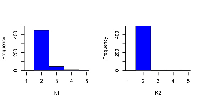
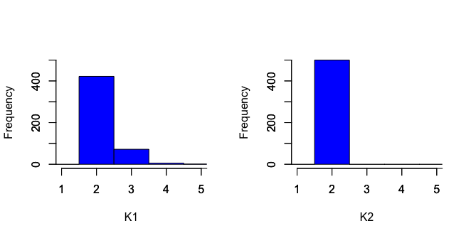
Table 1 reports the bias, standard deviation (Stdev), and the root mean square error (RMSE) of τ^\widehat{\tau} from the 500 Monte Carlo runs. In each Monte Carlo run, we use the data driven approach to select K1K_{1} and K2,K_{2}, and their histograms are depicted in Figure 1. The estimated asymptotic variances are reported in Table 2.

Glancing at these tables, we have the following observations:

  1. 1.

    The naive estimator has large bias. This is not surprising since it ignores the confounding effect.

  2. 2.

    The multiple robust estimators (mr) of Wang and Tchetgen Tchetgen (2017) has huge bias when some functionals are misspecified.

  3. 3.

    The bounded multiple robust estimator (b-mr) of Wang and Tchetgen Tchetgen (2017) is more robust than mr-estimator, but it still has a significant bias if some functionals are misspecified. And the bias does not valish as the sample size increases. Moreover, if all functionals are misspecified, the bias of b-mr estimator is substantially large.

  4. 4.

    The proposed estimator (cbe) is unbiased for both N=500N=500 and N=1000N=1000. Its performance (Bias, Stdev, RMSE) is comparable to Wang and Tchetgen Tchetgen (2017) ’s estimator when all functionals are correctly parameterized.

  5. 5.

    In variance estimation, both the multiple robust estimator (mr) and the bounded multiple robust estimator (b-mr) have large biases when some functionals are misspecified. In contrast, the proposed variance estimator is consistent.

  6. 6.

    The histograms in Figure 1 reveal that for both N=500N=500 and N=1000N=1000, K1=2K_{1}=2 and K2=2K_{2}=2 are most preferred, suggesting that the growing rate of K1K_{1} and K2K_{2} is slow, an observation consistent with Assumption 3.5.

Overall, the simulation results show that the proposed estimator out-performs the existing estimators.

7 Concluding Remarks

Most of the existing treatment effect literature on observational data assume that all confounders are observed and available to researchers. In applications, it is often the case that some confounders are not observed or not available. Wang and Tchetgen Tchetgen (2017) studied identification and estimation of the average treament effect when some confounders are not observed. They propose to parameterize five unknown functionals and show that their estimation is consistent when certain functionals are correctly specified and is efficient when all functionals are correctly specified. This paper proposes an alternative estimation. Unlike Wang and Tchetgen Tchetgen (2017), the proposed estimation does not parameterize any of the functionals and is always consistent. Moreover, the proposed estimator attains the semiparametric efficiency bound. A simple asymptotic variance estimator is presented, and a small scale simulation study suggests the practicality of the proposed procedure.

Our procedure only applies to the binary treatment with unmeasured confounders. However, other forms of treatment, such as multiple valued or continuous treatment, may arise in applications. Extension of the proposed methodology to those forms of treatment with unmeasured confounders is certainly of great interest. This extension shall be pursued in a future project.

References

  • (1)
  • Abadie (2003) Abadie, A. (2003): “Semiparametric instrumental variable estimation of treatment response models,” Journal of Econometrics, 113(2), 231–263.
  • Abadie, Angrist, and Imbens (2002) Abadie, A., J. Angrist, and G. Imbens (2002): “Instrumental Variables Estimates of the Effect of Subsidized Training on the Quantiles of Trainee Earnings,” Econometrica, 70(1), 91–117.
  • Angrist, Imbens, and Rubin (1996) Angrist, J. D., G. W. Imbens, and D. B. Rubin (1996): “Identification of Causal Effects Using Instrumental Variables (Disc: P456-472),” Publications of the American Statistical Association, 91(434), 444–455.
  • Chan, Yam, and Zhang (2016) Chan, K. C. G., S. C. P. Yam, and Z. Zhang (2016): “Globally efficient non-parametric inference of average treatment effects by empirical balancing calibration weighting,” Journal of the Royal Statistical Society: Series B (Statistical Methodology), 78(3), 673–700.
  • Chen (2007) Chen, X. (2007): “Large sample sieve estimation of semi-nonparametric models,” Handbook of econometrics, 6, 5549–5632.
  • Chen, Hong, and Tarozzi (2008) Chen, X., H. Hong, and A. Tarozzi (2008): “Semiparametric efficiency in GMM models with auxiliary data,” Ann. Statist., 36(2), 808–843.
  • Cheng, Small, Tan, and Have (2009) Cheng, J., D. S. Small, Z. Tan, and T. R. T. Have (2009): “Efficient nonparametric estimation of causal effects in randomized trials with noncompliance,” Biometrika, 96(1), 19–36.
  • Dehejia and Wahba (1999) Dehejia, R. H., and S. Wahba (1999): “Causal effects in nonexperimental studies: Reevaluating the evaluation of training programs,” Journal of the American statistical Association, 94(448), 1053–1062.
  • Hansen (1982) Hansen, L. (1982): “Large sample properties of generalized method of moments estimators,” Econometrica, 50, 1029–1054.
  • Hansen, Heaton, and Yaron (1996) Hansen, L., J. Heaton, and A. Yaron (1996): “Finite-sample properties of some alternative GMM estimators,” Journal of Business & Economic Statistics, 14(3), 262–280.
  • Heckman, Ichimura, and Todd (1998) Heckman, J. J., H. Ichimura, and P. Todd (1998): “Matching as an econometric evaluation estimator,” The review of economic studies, 65(2), 261–294.
  • Heckman, Ichimura, and Todd (1997) Heckman, J. J., H. Ichimura, and P. E. Todd (1997): “Matching as an econometric evaluation estimator: Evidence from evaluating a job training programme,” The review of economic studies, 64(4), 605–654.
  • Hirano, Imbens, and Ridder (2003) Hirano, K., G. Imbens, and G. Ridder (2003): “Efficient Estimation of Average Treatment Effects Using the Estimated Propensity Score,” Econometrica, 71(4), 1161–1189.
  • Imai and Ratkovic (2014) Imai, K., and M. Ratkovic (2014): “Covariate balancing propensity score,” J. R. Statist. Soc. B (Statistical Methodology), 76(1), 243–263.
  • Imbens, Newey, and Ridder (2006) Imbens, G., W. Newey, and G. Ridder (2006): “Mean-Squared-Error Calculations for Average Treatment Effects,” Unpublished manuscript, University of California Berkeley.
  • Imbens, Spady, and Johnson (1998) Imbens, G., R. Spady, and P. Johnson (1998): “Information Theoretic Approaches to Inference in Moment Condition Models,” Econometrica, 66(2), 333–357.
  • Imbens and Angrist (1994) Imbens, G. W., and J. D. Angrist (1994): “Identification and Estimation of Local Average Treatment Effects,” Econometrica, 62(2), 467–475.
  • Imbens and Rubin (2015) Imbens, G. W., and D. B. Rubin (2015): Causal inference in statistics, social, and biomedical sciences. Cambridge University Press.
  • Imbens and Wooldridge (2009) Imbens, G. W., and J. M. Wooldridge (2009): “Recent developments in the econometrics of program evaluation,” Journal of economic literature, 47(1), 5–86.
  • Kitamura and Stutzer (1997) Kitamura, Y., and M. Stutzer (1997): “An information-theoretic alternative to generalized method of moments estimation,” Econometrica, 65(4), 861–874.
  • Newey (1994) Newey, W. K. (1994): “The Asymptotic Variance of Semiparametric Estimators,” Econometrica, 62(6), 1349–1382.
  • Newey (1997)    (1997): “Convergence Rates and Asymptotic Normality for Series Estimators,” Journal of Econometrics, 79, 147–168.
  • Ogburn, Rotnitzky, and Robins (2015) Ogburn, E. L., A. Rotnitzky, and J. M. Robins (2015): “Doubly robust estimation of the local average treatment effect curve,” J R Stat Soc, 77(2), 373–396.
  • Owen (1988) Owen, A. (1988): “Empirical likelihood ratio confidence intervals for a single functional,” Biometrika, 75(2), 237–249.
  • Qin and Lawless (1994) Qin, J., and J. Lawless (1994): “Empirical likelihood and general estimating equations,” Ann. Statist., 22, 300–325.
  • Rosenbaum (1987) Rosenbaum, P. R. (1987): “Model-based direct adjustment,” J. Am. Statist. Ass., 82(398), 387–394.
  • Rosenbaum (2002)    (2002): “Observational studies,” in Observational studies, pp. 1–17. Springer.
  • Rosenbaum et al. (2002) Rosenbaum, P. R., et al. (2002): “Covariance adjustment in randomized experiments and observational studies,” Statistical Science, 17(3), 286–327.
  • Rosenbaum and Rubin (1983) Rosenbaum, P. R., and D. B. Rubin (1983): “The central role of the propensity score in observational studies for causal effects,” Biometrika, 70(1), 41–55.
  • Rosenbaum and Rubin (1984)    (1984): “Reducing bias in observational studies using subclassification on the propensity score,” J. Am. Statist. Ass., 79(387), 516–524.
  • Tan (2006) Tan, Z. (2006): “Regression and Weighting Methods for Causal Inference Using Instrumental Variables,” Publications of the American Statistical Association, 101(476), 1607–1618.
  • Tan (2010) Tan, Z. (2010): “Bounded, efficient and doubly robust estimation with inverse weighting,” Biometrika, 97(3), 661–682.
  • Tseng and Bertsekas (1987) Tseng, P., and D. P. Bertsekas (1987): “Relaxation methods for problems with strictly convex separable costs and linear constraints,” Mathematical Programming, 38(3), 303–321.
  • Wang and Tchetgen Tchetgen (2017) Wang, L., and E. Tchetgen Tchetgen (2017): “Bounded, efficient and multiply robust estimation of average treatment effects using instrumental variables,” Journal of the Royal Statistical Society: Series B (Statistical Methodology).
  • Yiu and Su (2018) Yiu, S., and L. Su (2018): “Covariate association eliminating weights: a unified weighting framework for causal effect estimation,” Biometrika.

Appendix A Appendix

A.1 Discussion on uKu_{K}

To construct our estimator, we need to specify the sieve basis uK(X)u_{K}(X). Although the approximation theory is derived for general sequences of sieve basis, the most common class of functions are power series and splines. In particular, we can approximate any function f:rf:\mathbb{R}^{r}\to\mathbb{R} by γ~Ku~K(x)\tilde{\gamma}_{K}^{\top}\tilde{u}_{K}(x), where u~K(x)\tilde{u}_{K}(x) is a prespecified sieve basis. Because γ~Ku~K(x)=γ~KAK×K1AK×Ku~K(x)\tilde{\gamma}^{\top}_{K}\tilde{u}_{K}(x)=\tilde{\gamma}_{K}^{\top}A_{K\times K}^{-1}A_{K\times K}\tilde{u}_{K}(x), we can also use uK(x)=AK×Ku~K(x)u_{K}(x)=A_{K\times K}\tilde{u}_{K}(x) as the new basis for approximation. By choosing AK×KA_{K\times K} appropriately we obtain a system of orthonormal basis (with respect to some weights). In particular, we choose AK×KA_{K\times K} so that

𝔼[uK(X)uK(X)]=IK×K.\displaystyle\mathbb{E}\left[u_{K}(X)u_{K}^{\top}(X)\right]=I_{K\times K}\ . (A.1)

We define the usual Frobenius norm Atr(AA)\|A\|\triangleq\sqrt{\text{tr}(AA^{\top})} for any matrix AA. Define

ζ(K)supx𝒳uK(x).\displaystyle\zeta(K)\triangleq\sup_{x\in\mathcal{X}}\|u_{K}(x)\|\ . (A.2)

In general, this bound depends on the array of basis that is used. Newey (1994, 1997) showed that

  1. 1.

    for power series: there exists a universal constant C0>0C_{0}>0 such that ζ(K)C0K\zeta(K)\leq C_{0}K;

  2. 2.

    for regression splines: there exists a universal constant C0>0C_{0}>0 such that ζ(K)C0K\zeta(K)\leq C_{0}\sqrt{K}.

A.2 Duality of Constrained Optimization

Let L(v,v0)L(v,v_{0}) be a distance measure that is continuously differentiable in vv\in\mathbb{R}, non-negative, strictly convex in vv and L(v0,v0)=0L(v_{0},v_{0})=0. The general idea of calibration is to minimize the aggregate distance between the final weights to a given vector of design weights subject to moment constraints. Being motivated by (3.4), we consider to construct the calibration weights {wi}i=1N\{w_{i}\}_{i=1}^{N} by solving the following constrained optimization problem:

{Minimizei=1NL(wi,1),subject to1Ni=1NZiwiuK1(Xi)=1Ni=1NuK1(Xi)=1Ni=1N(1Zi)wiuK1(Xi),\displaystyle\left\{\begin{array}[]{ll}&\qquad\qquad\qquad\qquad\text{Minimize}~~~\sum_{i=1}^{N}L(w_{i},1)\ ,\\[8.53581pt] &\text{subject to}~~\frac{1}{N}\sum_{i=1}^{N}Z_{i}w_{i}u_{K_{1}}({X}_{i})=\frac{1}{N}\sum_{i=1}^{N}u_{K_{1}}({X}_{i})=\frac{1}{N}\sum_{i=1}^{N}(1-Z_{i})w_{i}u_{K_{1}}({X}_{i})\end{array}\right.\ , (A.5)

where K1K_{1}\to\infty as the sample size NN\to\infty, yet with K1/N0K_{1}/N\to 0. The constrained optimization problem stated above is equivalent to two separate constrained optimization problems.

Minimizei=1NZiL(Npi,1)subject toi=1NZipiuK1(Xi)=1Ni=1NuK1(Xi),\displaystyle\text{Minimize}~~~\sum_{i=1}^{N}Z_{i}L(Np_{i},1)~~\text{subject to}~~\sum_{i=1}^{N}Z_{i}p_{i}u_{K_{1}}({X}_{i})=\frac{1}{N}\sum_{i=1}^{N}u_{K_{1}}({X}_{i})\ , (A.6)
Minimizei=1N(1Zi)L(Nqi,1)subject toi=1N(1Zi)qiuK1(Xi)=1Ni=1NuK1(Xi).\displaystyle\text{Minimize}~~~\sum_{i=1}^{N}(1-Z_{i})L(Nq_{i},1)~~\text{subject to}~~\sum_{i=1}^{N}(1-Z_{i})q_{i}u_{K_{1}}({X}_{i})=\frac{1}{N}\sum_{i=1}^{N}u_{K_{1}}({X}_{i})\ \ . (A.7)

Because the primal problems (A.6) and (A.7) are convex separable programs with linear constraints, Tseng and Bertsekas (1987) showed that the dual problems are unconstrained convex maximization problems that can be solved by numerical efficient and stable algorithms.

We show the dual of (A.6) is the unconstrained optimization (3.8) by using the methodology introduced in Tseng and Bertsekas (1987). Let g(v)=L(1v,1)g(v)=L(1-v,1), g(v)=g(v)/vg^{\prime}(v)=\partial g(v)/\partial v, EK1×N(uK1(X1),,uK1(XN))E_{K_{1}\times N}\triangleq\left(u_{K_{1}}(X_{1}),\ldots,u_{K_{1}}(X_{N})\right), si1ZiNpi,i=1,,Ns_{i}\triangleq 1-Z_{i}Np_{i},i=1,\ldots,N, and 𝐬(s1,,sN)\mathbf{s}\triangleq\left(s_{1},\ldots,s_{N}\right)^{\top}, then we can rewrite the problem (A.6) as

min𝐬i=1NZig(si)subject toEK1×N𝐬=0.\min_{\mathbf{s}}\sum_{i=1}^{N}Z_{i}g(s_{i})~~~\text{subject to}~~~~E_{K_{1}\times N}\cdot\mathbf{s}=0\ .

For every j{1,,N}j\in\{1,\ldots,N\}, we define the conjugate convex function (Tseng and Bertsekas, 1987) of Zjg()Z_{j}g(\cdot) to be

lj(uj)=\displaystyle l_{j}(u_{j})= supsj{ujsjZjg(sj)}=suppj{ZjNpjuj+ujZjg(1ZjNpj)}\displaystyle\sup_{s_{j}}\left\{u_{j}s_{j}-Z_{j}g(s_{j})\right\}=\sup_{p_{j}}\left\{-Z_{j}Np_{j}u_{j}+u_{j}-Z_{j}g(1-Z_{j}Np_{j})\right\}
=\displaystyle= suppj{ZjNpjuj+ujZjg(1Npj)}\displaystyle\sup_{p_{j}}\left\{-Z_{j}Np_{j}u_{j}+u_{j}-Z_{j}g(1-Np_{j})\right\}
=\displaystyle= ZjNpjuj+ujZjg(1Npj),\displaystyle-Z_{j}Np^{*}_{j}u_{j}+u_{j}-Z_{j}g(1-Np^{*}_{j})\ ,

where the third equality follows by Zg(1ZNpj)=Zg(1Npj)Zg(1-ZNp_{j})=Zg(1-Np_{j}), and pjp_{j}^{*} satisfies the first order condition:

Zjuj=Zjg(1Npj)pj=1N{1(g)1(uj)};\displaystyle-Z_{j}u_{j}=-Z_{j}g^{\prime}(1-Np_{j}^{*})\Rightarrow p_{j}^{*}=\frac{1}{N}\left\{1-\left(g^{\prime}\right)^{-1}(u_{j})\right\}\ ;

then we can have

lj(uj)=\displaystyle l_{j}(u_{j})= Zjuj{1(g)1(uj)}+ujZjg((g)1(uj))\displaystyle-Z_{j}u_{j}\left\{1-\left(g^{\prime}\right)^{-1}(u_{j})\right\}+u_{j}-Z_{j}g\left(\left(g^{\prime}\right)^{-1}(u_{j})\right)
=\displaystyle= Zj{g((g)1(uj))+ujuj(g)1(uj)}+uj\displaystyle-Z_{j}\left\{g\left(\left(g^{\prime}\right)^{-1}(u_{j})\right)+u_{j}-u_{j}\left(g^{\prime}\right)^{-1}(u_{j})\right\}+u_{j}
=\displaystyle= Zjρ(uj)+uj,\displaystyle-Z_{j}\rho\left(u_{j}\right)+u_{j}\ ,

where

ρ(u)g((g)1(u))+uu(g)1(u).\rho\left(u\right)\triangleq g\left(\left(g^{\prime}\right)^{-1}(u)\right)+u-u\left(g^{\prime}\right)^{-1}(u)\ .

By Tseng and Bertsekas (1987), the dual problem of (A.6) is

minλj=1Nlj(λEj)=minλj=1Nlj(λuK1(Xj))\displaystyle\min_{\lambda}\sum_{j=1}^{N}l_{j}(\lambda^{\top}E_{j})=\min_{\lambda}\sum_{j=1}^{N}l_{j}(\lambda^{\top}u_{K_{1}}(X_{j}))
=\displaystyle= minλj=1N{Zjρ(λuK1(Xj))+λuK1(Xj)}\displaystyle\min_{\lambda}\sum_{j=1}^{N}\left\{-Z_{j}\rho\left(\lambda^{\top}u_{K_{1}}(X_{j})\right)+\lambda^{\top}u_{K_{1}}(X_{j})\right\}
=\displaystyle= maxλj=1N{Zjρ(λuK1(Xj))λuK1(Xj)}\displaystyle-\max_{\lambda}\sum_{j=1}^{N}\left\{Z_{j}\rho\left(\lambda^{\top}u_{K_{1}}(X_{j})\right)-\lambda^{\top}u_{K_{1}}(X_{j})\right\}
=\displaystyle= maxλG^(λ),\displaystyle-\max_{\lambda}\hat{G}(\lambda)\ ,

where EjE_{j} is the jj-th column of EK1×NE_{K_{1}\times N}, i,e., Ej=uK1(Xj)E_{j}=u_{K_{1}}(X_{j}), which is our formulation (3.8).

Since L()L(\cdot) is strictly convex, i.e., L′′(v)>0L^{\prime\prime}(v)>0, and g′′(v)=L′′(1v)g^{\prime\prime}(v)=L^{\prime\prime}(1-v), then g()g(\cdot) is also strictly convex and g()g^{\prime}(\cdot) is strictly increasing. Note that

ρ(v)=g((g1(v))+vv(g1(v)ρ(g(v))=g(v)+g(v)vg(v).\displaystyle\rho(v)=g((g^{\prime-1}(v))+v-v(g^{\prime-1}(v)\Leftrightarrow\rho\left(g^{\prime}(v)\right)=g(v)+g^{\prime}(v)-vg^{\prime}(v)\ .

Differentiating vv on both sides in above equation yields:

ρ(g(v))g′′(v)=g(v)+g′′(v)g(v)vg′′(v)=(1v)g′′(v).\displaystyle\rho^{\prime}\left(g^{\prime}(v)\right)g^{\prime\prime}(v)=g^{\prime}(v)+g^{\prime\prime}(v)-g^{\prime}(v)-vg^{\prime\prime}(v)=(1-v)g^{\prime\prime}(v)\ .

Since g′′(v)>0g^{\prime\prime}(v)>0, we can have

ρ(g(v))=1v,\displaystyle\rho^{\prime}\left(g^{\prime}(v)\right)=1-v\ ,

then we differentiate vv on both sides to get ρ′′(g(v))g′′(v)=1\rho^{\prime\prime}\left(g^{\prime}(v)\right)g^{\prime\prime}(v)=-1, which implies

ρ′′(v)=1g′′((g1(v))<0.\rho^{\prime\prime}(v)=-\frac{1}{g^{\prime\prime}\left((g^{\prime-1}(v)\right)}<0\ .

Therefore, the convexity of L()L(\cdot) is equivalent to the concavity of ρ()\rho(\cdot).

A.3 Convergence Rates of Estimated Weights

The following result ensures the consistency of Np^(X)N\hat{p}(X), Nq^(X)N\hat{q}(X) and δ^D(X)\hat{\delta}^{D}(X) as well as their convergence rates. The proof is presented in Section 2 of the supplemental material.

Proposition A.1.

Under Assumptions 3.2-3.6, we have

supx𝒳|Np^(x)fZ|X(1|x)1|=Op(ζ(K)Kα+ζ(K)KN),\displaystyle\sup_{x\in\mathcal{X}}|N\hat{p}(x)-f_{Z|X}(1|x)^{-1}|=O_{p}\left(\zeta(K)K^{-\alpha}+\zeta(K)\sqrt{\frac{K}{N}}\right)\ ,
𝒳|Np^(x)fZ|X(1|x)1|2dFX(x)=Op(K2α+KN),\displaystyle\int_{\mathcal{X}}|N\hat{p}(x)-f_{Z|X}(1|x)^{-1}|^{2}dF_{X}(x)=O_{p}\left(K^{-2\alpha}+{\frac{K}{N}}\right)\ ,
1Ni=1N|Np^(Xi)fZ|X(1|Xi)1|2=Op(K2α+KN),\displaystyle\frac{1}{N}\sum_{i=1}^{N}|N\hat{p}(X_{i})-f_{Z|X}(1|X_{i})^{-1}|^{2}=O_{p}\left(K^{-2\alpha}+{\frac{K}{N}}\right)\ ,

and

supx𝒳|Nq^(x)fZ|X(0|x)1|=Op(ζ(K)Kα+ζ(K)KN),\displaystyle\sup_{x\in\mathcal{X}}|N\hat{q}(x)-f_{Z|X}(0|x)^{-1}|=O_{p}\left(\zeta(K)K^{-\alpha}+\zeta(K)\sqrt{\frac{K}{N}}\right)\ ,
𝒳|Nq^(x)fZ|X(0|x)1|2dFX(x)=Op(K2α+KN),\displaystyle\int_{\mathcal{X}}|N\hat{q}(x)-f_{Z|X}(0|x)^{-1}|^{2}dF_{X}(x)=O_{p}\left(K^{-2\alpha}+{\frac{K}{N}}\right)\ ,
1Ni=1N|Nq^(Xi)fZ|X(0|Xi)1|2=Op(K2α+KN),\displaystyle\frac{1}{N}\sum_{i=1}^{N}|N\hat{q}(X_{i})-f_{Z|X}(0|X_{i})^{-1}|^{2}=O_{p}\left(K^{-2\alpha}+{\frac{K}{N}}\right)\ ,

and

supx𝒳|δ^D(x)δD(x)|=Op(ζ(K)Kα+ζ(K)KN),\displaystyle\sup_{x\in\mathcal{X}}|\hat{\delta}^{D}(x)-\delta^{D}(x)|=O_{p}\left(\zeta(K)K^{-\alpha}+\zeta(K)\sqrt{\frac{K}{N}}\right)\ ,
𝒳|δ^D(x)δD(x)|2𝑑FX(x)=Op(K2α+KN),\displaystyle\int_{\mathcal{X}}|\hat{\delta}^{D}(x)-\delta^{D}(x)|^{2}dF_{X}(x)=O_{p}\left(K^{-2\alpha}+{\frac{K}{N}}\right)\ ,
1Ni=1N|δ^D(Xi)δD(Xi)|2=Op(K2α+KN).\displaystyle\frac{1}{N}\sum_{i=1}^{N}|\hat{\delta}^{D}(X_{i})-\delta^{D}(X_{i})|^{2}=O_{p}\left(K^{-2\alpha}+{\frac{K}{N}}\right)\ .

A.4 Sketched Proof of Theorem 3.7

The detailed proof of Theorem 3.7 is given in the supplementary material. Here we present the outline of whole the proof. By Assumption 3.5, K1K2KK_{1}\asymp K_{2}\asymp K, without loss of generality, we assume that K1=K2=KK_{1}=K_{2}=K. We introduce the following notation: let G(λ)G^{*}(\lambda), λK\lambda_{K}^{*} and p(X)p^{*}(X) be the theoretical counterparts of G^(λ)\hat{G}(\lambda), λ^K\hat{\lambda}_{K} and p^(X)\hat{p}(X) defined by

G(λ)=𝔼[G^K(λ)]=𝔼[Zρ(λuK(X))λuK(X)],\displaystyle G^{*}(\lambda)=\mathbb{E}[\hat{G}_{K}(\lambda)]=\mathbb{E}\left[Z\rho^{\prime}\left(\lambda^{\top}u_{K}(X)\right)-\lambda^{\top}u_{K}(X)\right]\ ,
λK=argmaxG(λ),p(X)=1Nρ((λK)uK(X)).\displaystyle\lambda_{K}^{*}=\arg\max G^{*}(\lambda)\ ,\ {p}^{*}(X)=\frac{1}{N}\rho^{\prime}(({\lambda}_{K}^{*})^{\top}u_{K}(X))\ .

We also introduce the following notation:

p1Y(X)=𝔼[Y|Z=1,X],p0Y(X)=𝔼[Y|Z=0,X],δY(X)=p1Y(X)p0Y(X),\displaystyle p^{Y}_{1}(X)=\mathbb{E}[Y|Z=1,X]\ ,\ p^{Y}_{0}(X)=\mathbb{E}[Y|Z=0,X]\ ,\ \delta^{Y}(X)=p^{Y}_{1}(X)-p^{Y}_{0}(X)\ ,
Ψ~K=𝒳p1Y(x)δD(x)fZ|X(1|x)ρ′′(λ~KuK(x))uK(x)𝑑FX(x),\displaystyle\tilde{\Psi}_{K}=-\int_{\mathcal{X}}\frac{p_{1}^{Y}(x)}{\delta^{D}(x)}f_{Z|X}(1|x)\rho^{\prime\prime}(\tilde{\lambda}_{K}^{\top}u_{K}(x))u_{K}(x)dF_{X}(x)\ ,
ΨK=𝒳p1Y(x)δD(x)fZ|X(1|x)ρ′′((λK)uK(x))uK(x)𝑑FX(x),\displaystyle{\Psi}_{K}=-\int_{\mathcal{X}}\frac{p_{1}^{Y}(x)}{\delta^{D}(x)}f_{Z|X}(1|x)\rho^{\prime\prime}(({\lambda}^{*}_{K})^{\top}u_{K}(x))u_{K}(x)dF_{X}(x)\ ,
Σ~K=1Ni=1NZiρ′′(λ~KuK(Xi))uK(Xi)uK(Xi),\displaystyle\tilde{\Sigma}_{K}=\frac{1}{N}\sum_{i=1}^{N}Z_{i}\rho^{\prime\prime}(\tilde{\lambda}_{K}^{\top}u_{K}(X_{i}))u_{K}(X_{i})u_{K}(X_{i})^{\top}\ ,
ΣK=𝔼[fZ|X(1|X)ρ′′((λK)uK(X))uK(X)uK(X)],\displaystyle\Sigma_{K}=-\mathbb{E}\left[f_{Z|X}(1|X)\rho^{\prime\prime}(({\lambda}_{K}^{*})^{\top}u_{K}(X))u_{K}(X)u_{K}(X)^{\top}\right]\ ,
Q~K(X)=Ψ~KΣ~K1uK(X),QK(X)=ΨKΣK1uK(X),\displaystyle\tilde{Q}_{K}(X)=\tilde{\Psi}_{K}^{\top}\tilde{\Sigma}_{K}^{-1}u_{K}(X)\ ,\ {Q}_{K}(X)={\Psi}_{K}^{\top}{\Sigma}_{K}^{-1}u_{K}(X)\ ,

where λ~K\tilde{\lambda}_{K} lies on the line joining λ^K\hat{\lambda}_{K} and λK\lambda_{K}^{*}. Note that QK(X)Q_{K}(X) is the weighted L2L^{2} projection of p1Y(X)/δD(X)-p^{Y}_{1}(X)/\delta^{D}(X) on the space linearly spanned by uK(X)u_{K}(X). Note that

N(τ^τ)=Ni=1NZip^(Xi)Yi/δ^D(Xi)Ni=1N(1Zi)q^(Xi)Yi/δ^D(Xi).\sqrt{N}(\hat{\tau}-\tau)=\sqrt{N}\sum_{i=1}^{N}Z_{i}\hat{p}(X_{i})Y_{i}/\hat{\delta}^{D}(X_{i})-\sqrt{N}\sum_{i=1}^{N}(1-Z_{i})\hat{q}(X_{i})Y_{i}/\hat{\delta}^{D}(X_{i})\ .

We first derive the influence function of Ni=1NZip^(Xi)Yi/δ^D(Xi)\sqrt{N}\sum_{i=1}^{N}Z_{i}\hat{p}(X_{i})Y_{i}/\hat{\delta}^{D}(X_{i}), and similarly obtain that of Ni=1N(1Zi)q^(Xi)Yi/δ^D(Xi)\sqrt{N}\sum_{i=1}^{N}(1-Z_{i})\hat{q}(X_{i})Y_{i}/\hat{\delta}^{D}(X_{i}). We can decompose Ni=1NZip^(Xi)Yi/δ^D(Xi)\sqrt{N}\sum_{i=1}^{N}Z_{i}\hat{p}(X_{i})Y_{i}/\hat{\delta}^{D}(X_{i}) as follows:

Ni=1NZip^(Xi)Yi/δ^D(Xi)\displaystyle\sqrt{N}\sum_{i=1}^{N}Z_{i}\hat{p}(X_{i})Y_{i}/\hat{\delta}^{D}(X_{i})
=\displaystyle= 1Ni=1NZiδ^D(Xi){Np^(Xi)Np(Xi)}Yi1Ni=1NZiδD(Xi){Np^(Xi)Np(Xi)}Yi\displaystyle\frac{1}{\sqrt{N}}\sum_{i=1}^{N}\frac{Z_{i}}{\hat{\delta}^{D}(X_{i})}\{N\hat{p}(X_{i})-N{p}^{*}(X_{i})\}Y_{i}-\frac{1}{\sqrt{N}}\sum_{i=1}^{N}\frac{Z_{i}}{\delta^{D}(X_{i})}\{N\hat{p}(X_{i})-N{p}^{*}(X_{i})\}Y_{i} (A.8)
+1Ni=1NZiδ^D(Xi)Np(Xi)Yi1Ni=1NZiδD(Xi)Np(Xi)Yi\displaystyle+\frac{1}{\sqrt{N}}\sum_{i=1}^{N}\frac{Z_{i}}{\hat{\delta}^{D}(X_{i})}N{p}^{*}(X_{i})Y_{i}-\frac{1}{\sqrt{N}}\sum_{i=1}^{N}\frac{Z_{i}}{\delta^{D}(X_{i})}N{p}^{*}(X_{i})Y_{i} (A.9)
+1Ni=1N{ZiδD(Xi)(Np^(Xi)Np(Xi))Yi𝒳p1Y(x)fZ|X(1|x)δD(x)(Np^(X)Np(X))𝑑FX(x)}\displaystyle~+\frac{1}{\sqrt{N}}\sum_{i=1}^{N}\Bigg{\{}\frac{Z_{i}}{\delta^{D}(X_{i})}\left(N\hat{p}(X_{i})-Np^{*}(X_{i})\right)Y_{i}-\int_{\mathcal{X}}\frac{p_{1}^{Y}(x)f_{Z|X}(1|x)}{\delta^{D}(x)}(N\hat{p}(X)-Np^{*}(X))dF_{X}(x)\Bigg{\}} (A.10)
+1Ni=1N{(Np(Xi)1fZ|X(1|Xi))ZiYiδD(Xi)𝔼[p1Y(X)δD(X)fZ|X(1|X)(Np(X)1fZ|X(1|X))]}\displaystyle~+\frac{1}{\sqrt{N}}\sum_{i=1}^{N}\Bigg{\{}\left(Np^{*}(X_{i})-\frac{1}{f_{Z|X}(1|X_{i})}\right)\frac{Z_{i}Y_{i}}{\delta^{D}(X_{i})}-\mathbb{E}\left[\frac{p_{1}^{Y}(X)}{\delta^{D}(X)}f_{Z|X}(1|X)\left(Np^{*}(X)-\frac{1}{f_{Z|X}(1|X)}\right)\right]\Bigg{\}} (A.11)
+N𝔼[p1Y(X)δD(X)fZ|X(1|X)(Np(X)1fZ|X(1|X))]\displaystyle~+\sqrt{N}\mathbb{E}\left[\frac{p_{1}^{Y}(X)}{\delta^{D}(X)}f_{Z|X}(1|X)\left(Np^{*}(X)-\frac{1}{f_{Z|X}(1|X)}\right)\right] (A.12)
+N𝒳p1Y(x)δD(x)fZ|X(1|x)(Np^(X)Np(X))𝑑FX(x)1Ni=1N[Ziρ((λK)uK(Xi))1]Q~K(Xi)\displaystyle~+\sqrt{N}\int_{\mathcal{X}}\frac{p_{1}^{Y}(x)}{\delta^{D}(x)}f_{Z|X}(1|x)(N\hat{p}(X)-Np^{*}(X))dF_{X}(x)-\frac{1}{\sqrt{N}}\sum_{i=1}^{N}[Z_{i}\rho^{\prime}((\lambda_{K}^{*})^{\top}u_{K}(X_{i}))-1]\tilde{Q}_{K}(X_{i}) (A.13)
+1Ni=1N[Ziρ((λK)uK(Xi))1](Q~K(Xi)QK(Xi))\displaystyle~+\frac{1}{\sqrt{N}}\sum_{i=1}^{N}[Z_{i}\rho^{\prime}((\lambda_{K}^{*})^{\top}u_{K}(X_{i}))-1](\tilde{Q}_{K}(X_{i})-Q_{K}(X_{i})) (A.14)
+1Ni=1N{[Ziρ((λK)uK(Xi))1]QK(Xi)+p1Y(Xi)δD(Xi)(ZifZ|X(1|Xi)1)}\displaystyle~+\frac{1}{\sqrt{N}}\sum_{i=1}^{N}\left\{[Z_{i}\rho^{\prime}((\lambda_{K}^{*})^{\top}u_{K}(X_{i}))-1]Q_{K}(X_{i})+\frac{p_{1}^{Y}(X_{i})}{\delta^{D}(X_{i})}\left(\frac{Z_{i}}{f_{Z|X}(1|X_{i})}-1\right)\right\} (A.15)
+1Ni=1N{ZiYifZ|X(1|Xi)δD(Xi)p1Y(Xi)δD(Xi)(ZifZ|X(1|Xi)1)}.\displaystyle~+\frac{1}{\sqrt{N}}\sum_{i=1}^{N}\left\{\frac{Z_{i}Y_{i}}{f_{Z|X}(1|X_{i})\delta^{D}(X_{i})}-\frac{p_{1}^{Y}(X_{i})}{\delta^{D}(X_{i})}\left(\frac{Z_{i}}{f_{Z|X}(1|X_{i})}-1\right)\right\}\ . (A.16)

The following lemmas are proved in the supplemental material.

Lemma A.2.

Under Assumptions 3.1-3.6, the terms (A.8) (A.10), (A.11), (A.12), (A.13), (A.14) and (A.15) are of op(1)o_{p}(1)

Lemma A.3.

Under Assumptions 3.1-3.6, (A.9) has the following equivalent linear expression:

(A.9)=1Ni=1NDi2Zi1fZ|X(Zi|Xi)p1Y(Xi)δD(Xi)2+1Ni=1N2Zi1δD(Xi)2𝔼[Di|Zi,Xi]fZ|X(Zi|Xi)p1Y(Xi)+op(1).\displaystyle\eqref{eq:delta^-delta}=-\frac{1}{\sqrt{N}}\sum_{i=1}^{N}D_{i}\cdot\frac{2Z_{i}-1}{f_{Z|X}(Z_{i}|X_{i})}\cdot\frac{p_{1}^{Y}(X_{i})}{\delta^{D}(X_{i})^{2}}+\frac{1}{\sqrt{N}}\sum_{i=1}^{N}\frac{2Z_{i}-1}{\delta^{D}(X_{i})^{2}}\cdot\frac{\mathbb{E}[D_{i}|Z_{i},X_{i}]}{f_{Z|X}(Z_{i}|X_{i})}p_{1}^{Y}(X_{i})+o_{p}(1)\ .

By Lemmas A.2 and A.3, we can obtain that

Ni=1NZip^(Xi)Yi/δ^D(Xi)\displaystyle\sqrt{N}\sum_{i=1}^{N}Z_{i}\hat{p}(X_{i})Y_{i}/\hat{\delta}^{D}(X_{i})
=\displaystyle= 1Ni=1N{ZiYifZ|X(1|Xi)δD(Xi)p1Y(Xi)δD(Xi)(ZifZ|X(1|Xi)1)}\displaystyle\frac{1}{\sqrt{N}}\sum_{i=1}^{N}\left\{\frac{Z_{i}Y_{i}}{f_{Z|X}(1|X_{i})\delta^{D}(X_{i})}-\frac{p_{1}^{Y}(X_{i})}{\delta^{D}(X_{i})}\left(\frac{Z_{i}}{f_{Z|X}(1|X_{i})}-1\right)\right\}
1Ni=1NDi2Zi1fZ|X(Zi|Xi)p1Y(Xi)δD(Xi)2+1Ni=1N2Zi1δD(Xi)2𝔼[Di|Zi,Xi]fZ|X(Zi|Xi)p1Y(Xi)+op(1).\displaystyle-\frac{1}{\sqrt{N}}\sum_{i=1}^{N}D_{i}\cdot\frac{2Z_{i}-1}{f_{Z|X}(Z_{i}|X_{i})}\cdot\frac{p_{1}^{Y}(X_{i})}{\delta^{D}(X_{i})^{2}}+\frac{1}{\sqrt{N}}\sum_{i=1}^{N}\frac{2Z_{i}-1}{\delta^{D}(X_{i})^{2}}\cdot\frac{\mathbb{E}[D_{i}|Z_{i},X_{i}]}{f_{Z|X}(Z_{i}|X_{i})}p_{1}^{Y}(X_{i})+o_{p}(1)\ .

Symmetrically, we have

Ni=1N(1Zi)q^(Xi)Yi/δ^D(Xi)\displaystyle\sqrt{N}\sum_{i=1}^{N}(1-Z_{i})\hat{q}(X_{i})Y_{i}/\hat{\delta}^{D}(X_{i})
=\displaystyle= 1Ni=1N{(1Zi)YifZ|X(0|Xi)δD(Xi)p0Y(Xi)δD(Xi)(1ZifZ|X(0|Xi)1)}\displaystyle\frac{1}{\sqrt{N}}\sum_{i=1}^{N}\left\{\frac{(1-Z_{i})Y_{i}}{f_{Z|X}(0|X_{i})\delta^{D}(X_{i})}-\frac{p^{Y}_{0}(X_{i})}{\delta^{D}(X_{i})}\left(\frac{1-Z_{i}}{f_{Z|X}(0|X_{i})}-1\right)\right\}
1Ni=1NDi2Zi1fZ|X(Zi|Xi)p0Y(Xi)δD(Xi)2+1Ni=1N2Zi1δD(Xi)2𝔼[Di|Zi,Xi]fZ|X(Zi|Xi)p0Y(Xi)+op(1).\displaystyle-\frac{1}{\sqrt{N}}\sum_{i=1}^{N}D_{i}\cdot\frac{2Z_{i}-1}{f_{Z|X}(Z_{i}|X_{i})}\cdot\frac{p^{Y}_{0}(X_{i})}{\delta^{D}(X_{i})^{2}}+\frac{1}{\sqrt{N}}\sum_{i=1}^{N}\frac{2Z_{i}-1}{\delta^{D}(X_{i})^{2}}\cdot\frac{\mathbb{E}[D_{i}|Z_{i},X_{i}]}{f_{Z|X}(Z_{i}|X_{i})}p^{Y}_{0}(X_{i})+o_{p}(1)\ .

Therefore,

N(τ^τ)=Ni=1N{Zip^(Xi)δ^D(Xi)Yi(1Zi)q^(Xi)δ^D(Xi)Yiτ}\displaystyle\sqrt{N}(\hat{\tau}-\tau)=\sqrt{N}\sum_{i=1}^{N}\left\{Z_{i}\frac{\hat{p}(X_{i})}{\hat{\delta}^{D}(X_{i})}Y_{i}-(1-Z_{i})\frac{\hat{q}(X_{i})}{\hat{\delta}^{D}(X_{i})}Y_{i}-\tau\right\}
=\displaystyle= 1Ni=1N[2Zi1δD(Xi)fZ|X(Zi|Xi)Yiτ]\displaystyle\frac{1}{\sqrt{N}}\sum_{i=1}^{N}\bigg{[}\frac{2Z_{i}-1}{\delta^{D}(X_{i})f_{Z|X}(Z_{i}|X_{i})}Y_{i}-\tau\bigg{]}
1Ni=1Np1Y(Xi)δD(X){ZifZ|X(1|Xi)1}\displaystyle-\frac{1}{\sqrt{N}}\sum_{i=1}^{N}\frac{p_{1}^{Y}(X_{i})}{\delta^{D}(X)}\bigg{\{}\frac{Z_{i}}{f_{Z|X}(1|X_{i})}-1\bigg{\}}
+1Ni=1Np0Y(Xi)δD(X){1ZifZ|X(0|Xi)1}\displaystyle+\frac{1}{\sqrt{N}}\sum_{i=1}^{N}\frac{p_{0}^{Y}(X_{i})}{\delta^{D}(X)}\bigg{\{}\frac{1-Z_{i}}{f_{Z|X}(0|X_{i})}-1\bigg{\}}
1Ni=1Nδ(Xi){2Zi1fZ|X(Z|Xi)DiδD(Xi)2Zi1fZ|X(Z|Xi)𝔼[Di|Zi,Xi]δD(Xi)}+op(1)[sinceδ(X)=δY(X)δD(X)]\displaystyle-\frac{1}{\sqrt{N}}\sum_{i=1}^{N}\delta(X_{i})\bigg{\{}\frac{2Z_{i}-1}{f_{Z|X}(Z|X_{i})}\frac{D_{i}}{\delta^{D}(X_{i})}-\frac{2Z_{i}-1}{f_{Z|X}(Z|X_{i})}\frac{\mathbb{E}[D_{i}|Z_{i},X_{i}]}{\delta^{D}(X_{i})}\bigg{\}}+o_{p}(1)\quad\left[\text{since}\ \delta(X)=\frac{\delta^{Y}(X)}{\delta^{D}(X)}\right]
=\displaystyle= 1Ni=1Nφeff(Di,Zi,Xi,Yi)+op(1)\displaystyle\frac{1}{\sqrt{N}}\sum_{i=1}^{N}\varphi_{eff}(D_{i},Z_{i},X_{i},Y_{i})+o_{p}(1)

where

φeff(Di,Zi,Xi,Yi)=\displaystyle\varphi_{eff}(D_{i},Z_{i},X_{i},Y_{i})= 2Zi1fZ|X(Zi|Xi)1δD(Xi){YiDiδ(Xi)𝔼[Yi|Zi=0,Xi]+𝔼[Di|Zi=0,Xi]δ(Xi)}+δ(Xi)τ,\displaystyle\frac{2Z_{i}-1}{f_{Z|X}(Z_{i}|X_{i})}\frac{1}{\delta^{D}(X_{i})}\bigg{\{}Y_{i}-D_{i}\delta(X_{i})-\mathbb{E}[Y_{i}|Z_{i}=0,X_{i}]+\mathbb{E}[D_{i}|Z_{i}=0,X_{i}]\delta(X_{i})\bigg{\}}+\delta(X_{i})-\tau\ ,

is the efficient influence function given in Wang and Tchetgen Tchetgen (2017).