A Small-Gain Theorem for Discrete-Time Convergent Systems and Its Applications

Jiayin Chen and Hendra I. Nurdin J. Chen and H. I. Nurdin are with the School of Electrical Engineering and Telecommunications, UNSW Australia, Sydney NSW 2052, Australia (email: jiayin.chen@unsw.edu.au, h.nurdin@unsw.edu.au)

Abstract

Convergent, contractive or incremental stability properties of nonlinear systems have attracted interest for control tasks such as observer design, output regulation and synchronization. The convergence property plays a central role in the neuromorphic (brain-inspired) computing of reservoir computing, which seeks to harness the information processing capability of nonlinear systems. This paper presents a small-gain theorem for discrete-time output-feedback interconnected systems to be uniformly input-to-output convergent (UIOC) with outputs converging to a bounded reference output uniquely determined by the input. A small-gain theorem for interconnected time-varying discrete-time uniform input-to-output stable systems that could be of separate interest is also presented as an intermediate result. Applications of the UIOC small-gain theorem are illustrated in the design of observer-based controllers and interconnected nonlinear classical and quantum dynamical systems (as reservoir computers) for black-box system identification.

Index Terms:

Convergent dynamics; Reservoir computing; Small-gain; Input-to-output stability.

I Introduction

Convergence notions, such as incremental stability [1], convergent dynamics [2, 3] and contracting dynamics [4], impose that all solutions must “forget” their initial conditions and converge to each other asymptotically; also see [5] for a survey of such convergence properties in the discrete-time setting. Such properties have found applications in observer design [1, 4], output regulation [6, 7] and synchronization [1, 8].

In an independent development, efforts to go beyond the von Neumann computing architecture to imitate human capabilities in tasks that are difficult or energetically expensive on conventional digital computers, have led to the pursuit of neuromorphic (brain-inspired) computing paradigms implemented on physical hardware. Central to this is to exploit high-dimensional nonlinear dynamical systems for processing of time-varying input signals. An emerging neuromorphic paradigm is reservoir computing (RC) [9, 10], which uses a fixed but otherwise almost arbitrary dynamical system, the so-called “reservoir”, to map inputs into its state-space. This paper is interested in discrete-time reservoir computers (also abbreviated as RCs) that perform causal nonlinear operations on input sequences to produce output sequences. Only a simple linear regression algorithm is required to optimize the parameters of a readout function to approximate target output sequences. In the RC paradigm, convergence (referred to as the echo-state property in the RC literature) ensures that the reservoir outputs are asymptotically independent of its initial condition, and the reservoir induces an input-output (I/O) map to approximate a target I/O map [11].

A prominent example of RCs are the echo state networks (ESNs), which have demonstrated remarkable ability to predict chaotic time series [12, 13]. There is substantial interest in hardware realizations of RC for fast processing using less memory and energy, as opposed to software-based implementation on digital computers. For instance, a photonic RC achieved high-speed speech classification (million words per second) with low error rates [14] and a FPGA-based RC reached an 160 MHz rate for time-series prediction [15]; see [16, 17, 18] for other recent RC hardware implementations. Its extremely efficient training makes RC suitable for applications such as edge computing, in which information processing is incorporated into decentralized sensors (the ‘edges’) to reduce computation and transmission overhead [19]. For more recent developments, see [9, 10, 19].

Recent years have also seen the advent of noisy near-term intermediate scale quantum (NISQ) computers [20], which are not equipped with quantum error correction and can only perform a limited form of quantum computing, made available via cloud-based access from companies such as IBM [21]. This has led to the proposal of RCs that exploit nonlinear quantum dynamics (referred to as QRC) [22, 23]. Control-oriented applications of QRCs were put forward in [24] and Ref. [25] further develops a QRC scheme that can be implemented on NISQ computers and demonstrates a proof-of-principle of QRC on cloud-based IBM superconducting quantum computers [21]. This work provides further theoretical support for the application of RC and QRC for black-box system identification of discrete-time nonlinear systems, with examples developed in Section IV. Since QRCs can have a high-dimensional underlying Hilbert space, it may be advantageous for identifying systems with a high-dimensional state-space.

This paper focuses on uniformly convergent dynamics or the uniform convergence (UC) property. For output-feedback interconnected systems, we introduce the uniform output convergence (UOC) and the uniform input-to-output convergence (UIOC) properties. Roughly speaking, a UOC system has a unique reference state solution with its reference output defined and bounded both backwards and forwards in time. All other outputs asymptotically converge to the reference output, independent of their initial conditions. The UIOC property adapts the uniform input-to-state convergence (UISC) property [2] to output-feedback interconnected systems. A UIOC system is UOC and the perturbation in its reference outputs are asymptotically bounded by a nonlinear gain on the input perturbation. We present a small-gain theorem for output-feedback interconnected systems to be UIOC, and that the closed-loop system induces a well-posed I/O map in the sense of [26].

Our UIOC small-gain theorem is based on a small-gain theorem for time-varying discrete-time systems in the uniform input-to-output stability (UIOS) framework, also presented herein. This latter small-gain result is used to establish the UIOC small-gain theorem for interconnected time-invariant UOC systems, the time-variance arising through a change of variables. Small-gain criteria for time-varying continuous-time interconnected systems in the UIOS framework have been established [27, 28, 29, 30]. Ref. [31] develops a generalized small-gain theorem that recover the previous results for specific interconnections. Small-gain criteria for time-invariant discrete-time systems can be found in [32, 33]. Here, we adopt the techniques in [31] to establish a UIOS small-gain theorem for output-feedback interconnected time-varying discrete-time systems. Ref. [29] is based on [34, Lemma 3, Prop. 2.5], which also concerns continuous-time systems, and is not immediately applicable to our setting. Furthermore, [32, 33] do not carry over to time-varying systems [35]. Therefore, we establish a link to bridge our setting with the continuous-time results of [31].

Finally, we apply our results to observer-based controller design for globally Lipschitz systems [36, 37] and to design RC parameters for black-box system identification of discrete-time nonlinear systems solely based on I/O data collected from a system. Example nonlinear models for black-box system identification include NARMAX [38], the Volterra series [39] and block-oriented models [40, 41]. The use of closed-loop structures, such as in the Wiener-Hammerstein feedback model, is motivated by modeling systems that exhibit nonlinear feedback behavior [41]. Here we introduce interconnected ESNs and QRCs as models with closed-loop structures. The interconnected ESNs and QRCs dynamics are arbitrary but fixed at the onset, as long as they satisfy the UIOC small-gain theorem. Only an RC output function is optimized via ordinary least squares to fit the data, making the RC approach computationally efficient. We illustrate numerically the efficacy of this approach to model a feedback-controlled nonlinear system.

Notation. $\|\cdot\|$ is the Euclidean norm. $\mathbb{Z}$ $(\mathbb{R})$ and $\mathbb{Z}_{\geq k_{0}}$ ( $\mathbb{R}_{\geq k_{0}}$ ) denote, respectively, integers (reals) and integers (reals) larger than equal to $k_{0}\in\mathbb{Z}$ . $x\in\mathbb{R}^{n}$ is a column vector and $x^{\top}$ its transpose. For $x_{j}\in\mathbb{R}^{n_{j}}(j=1,2)$ , $(x_{1},x_{2})\in\mathbb{R}^{n_{1}+n_{2}}$ is their concatenation into a column vector. For a sequence $z$ on $\mathbb{Z}$ , $\|z_{[k_{0},k]}\|\coloneqq\sup_{k_{0}\leq j\leq k}\|z(j)\|$ for any $k_{0}\in\mathbb{Z}$ and $k\geq k_{0}$ . $l_{n}^{\infty}$ denotes the set of bounded sequences on $\mathbb{Z}$ , i.e., $z\in l^{\infty}_{n}$ if $z(k)\in\mathbb{R}^{n}$ and $\|z\|_{\infty}\coloneqq\sup_{k\in\mathbb{Z}}\|z(k)\|<\infty$ . For any sequences $z_{1},z_{2}$ on $\mathbb{Z}$ , $z=(z_{1},z_{2})$ is given by $z(k)=(z_{1}(k),z_{2}(k))$ $\forall k\in\mathbb{Z}$ . Function composition is denoted by $\circ$ . We use standard comparison function classes $\mathcal{K},\mathcal{K_{\infty}}$ and $\mathcal{KL}$ [28]¹¹1A function $\gamma:\mathbb{R}_{\geq 0}\rightarrow\mathbb{R}_{\geq 0}$ is a $\mathcal{K}$ function if it is continuous, strictly increasing and $\gamma(0)=0$ . A $\mathcal{K}$ function is a $\mathcal{K}_{\infty}$ function if it is unbounded. A $\mathcal{KL}$ function $\beta:\mathbb{R}_{\geq 0}\times\mathbb{R}_{\geq 0}\rightarrow\mathbb{R}_{\geq 0}$ is $\mathcal{K}$ in the first argument and decreasing (i.e., non-increasing) in the second argument, with $\lim_{t\rightarrow\infty}\beta(s,t)=0$ for all $s\in\mathbb{R}_{\geq 0}$ . As in [28, 42], we do not require a $\mathcal{KL}$ function to be continuous or strictly decreasing in the second argument..

II Stability concepts

This section defines the uniform output convergence (UOC) (Def. 2) and the uniform input-to-output convergence (UIOC) (Def. 4) properties. See Table I for a summary of relevant stability definitions. We first set some preliminaries.

For $k\in\mathbb{Z}$ , consider a time-varying discrete-time system,

\begin{cases}x(k+1)=f(k,x(k),u(k)),\\ \hskip 18.00005pty(k)=h(k,x(k),u(k)),\end{cases}

(1)

where $x(k)\in\mathbb{R}^{n_{x}}$ is the state, $u(k)\in\mathbb{R}^{n_{u}}$ is the input and $y(k)\in\mathbb{R}^{n_{y}}$ is the output. We assume that $u\in l^{\infty}_{n_{u}}$ and for each $k\in\mathbb{Z}$ , $\|f(k,x(k),u(k))\|<\infty$ and $\|h(k,x(k),u(k))\|<\infty$ . These conditions ensure that the system is non-singular at any time and for any initial condition.

The following definition of UOC adapts the uniform convergence (UC) property [5, Def. 3] to systems with output of the form (1).

Definition 1

For any $u\in l_{n_{u}}^{\infty}$ , a solution $x^{*}(k)$ to (1) and its corresponding output $y^{*}(k)=h(k,x^{*}(k),u(k))$ are a reference state solution and the corresponding reference output, respectively, if they are defined for all $k\in\mathbb{Z}$ , with $\|x^{*}\|_{\infty}<\infty$ and $\|y^{*}\|_{\infty}<\infty$ .

Definition 2

System (1) is uniformly output convergent (UOC) if, for any input $u\in l^{\infty}_{n_{u}}$ ,

(i)

There exists a unique reference state solution $x^{*}$ with its corresponding reference output $y^{*}$ .
(ii)

There exists $\beta\in\mathcal{KL}$ independent of $u$ such that, for any $k,k_{0}\in\mathbb{Z}$ with $k\geq k_{0}$ and $x(k_{0})\in\mathbb{R}^{n_{x}}$ ,

\|y^{*}(k)-y(k)\|\leq\beta(\|x^{*}(k_{0})-x(k_{0})\|,k-k_{0}).

(2)

System (1) with $y(k)=x(k)$ is uniformly convergent (UC) if, for any $u\in l^{\infty}_{n_{u}}$ ,

(i)

There exists a unique reference state solution $x^{*}$ .
(ii)

There exists $\beta\in\mathcal{KL}$ independent of $u$ such that, for any $k,k_{0}\in\mathbb{Z}$ with $k\geq k_{0}$ and $x(k_{0})\in\mathbb{R}^{n_{x}}$ ,

\|x^{*}(k)-x(k)\|\leq\beta(\|x^{*}(k_{0})-x(k_{0})\|,k-k_{0}).

(3)

Remark 3

In this note, all gain functions (e.g. $\beta$ in (2) and (3)) are independent of the input $u\in l_{n_{u}}^{\infty}$ . Further, as in [5], ‘uniform’ means that for each $x(k_{0})$ , the bound $\beta(\|x(k_{0})\|,k-k_{0})$ in (2) and (3) depends on $k-k_{0}$ but not $k_{0}$ .

The UIOC property further extends the UOC property, and ensures that the perturbation in the reference outputs is asymptotically bounded by a nonlinear gain of the input perturbation. The following definition of UIOC is a discrete-time analogue of the UISC property defined in [2, Def. 3] adapted to systems with output of the form (1).

Definition 4

System (1) is uniformly input-to-output convergent (UIOC) if it is UOC and for any $u,\overline{u}\in l^{\infty}_{n_{u}}$ , with the reference state solution $x^{*}$ and its reference output $y^{*}$ associated to $u$ , and any solution $\overline{x}(k)$ with any initial condition $\overline{x}(k_{0})$ and the corresponding output $\overline{y}(k)$ associated to $\overline{u}$ , there exists $\beta\in\mathcal{KL},\gamma\in\mathcal{K}$ such that, for all $k_{0},k\in\mathbb{Z}$ with $k\geq k_{0}$ ,

\begin{split}\|y^{*}(k)-\overline{y}(k)\|\leq\max\{\beta(\|x^{*}(k_{0})-\overline{x}(k_{0})\|,k-k_{0}),&\\ \gamma\left(\|(u-\overline{u})_{[k_{0},k]}\|\right)\}.&\end{split}

(4)

System (1) with $y(k)=x(k)$ is uniformly input-to-state convergent (UISC) if it is UC and

\begin{split}\|x^{*}(k)-\overline{x}(k)\|\leq\max\{\beta(\|x^{*}(k_{0})-\overline{x}(k_{0})\|,k-k_{0}),&\\ \gamma\left(\|(u-\overline{u})_{[k_{0},k-1]}\|\right)\}.&\end{split}

(5)

We conclude this section by summarizing the aforementioned stability concepts and their acronyms in Table I.

TABLE I: Summary of stability concepts and their acronyms.

Stability concept	Acronym	Definition
Uniformly output convergent	UOC	Definition 2
Uniformly convergent	UC	Definition 2
Uniformly input-to-output convergent	UIOC	Definition 4
Uniformly input-to-state convergent	UISC	Definition 4

III A UIOC small-gain theorem

In this section, we present our main UIOC small-gain theorem (Theorem 5). We first set some preliminaries.

For $k\in\mathbb{Z}$ , consider the interconnected system (see Fig. 1),

\begin{split}&\begin{cases}x_{1}(k+1)=f_{1}(x_{1}(k),v_{1}(k),u_{1}(k))\\ \hskip 18.00005pty_{1}(k)=h_{1}(x_{1}(k),v_{1}(k),u_{1}(k)),\\ \end{cases}\\ &\begin{cases}x_{2}(k+1)=f_{2}(x_{2}(k),v_{2}(k),u_{2}(k))\\ \hskip 18.00005pty_{2}(k)=h_{2}(x_{2}(k),v_{2}(k),u_{2}(k)),\\ \end{cases}\\ &\qquad v_{1}(k)=y_{2}(k),\ v_{2}(k)=y_{1}(k).\end{split}

(6)

Figure 1: Schematic of the interconnected system (6).

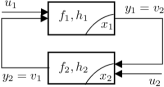
For subsystems $j=1,2$ , $x_{j}(k)\in\mathbb{R}^{n_{x_{j}}}$ are states, $y_{j}(k)\in\mathbb{R}^{n_{y_{j}}}$ are outputs and $u_{j}(k)\in\mathbb{R}^{n_{u_{j}}}$ are inputs with $u_{j}\in l^{\infty}_{n_{u_{j}}}$ . Throughout, we assume that the interconnected system (6) is well-posed. That is, for any $k,k_{0}\in\mathbb{Z}$ with $k\geq k_{0}$ and any initial conditions $x_{j}(k_{0})$ , there exists a unique solution $y(k)\coloneqq(y_{1}(k),y_{2}(k))\in\mathbb{R}^{n_{y_{1}}+n_{y_{2}}}$ solving the algebraic equations $y_{1}(k)=h_{1}(x_{1}(k),y_{2}(k),u_{1}(k))$ and $y_{2}(k)=h_{2}(x_{2}(k),y_{1}(k),u_{2}(k))$ .

For a well-posed system (6), let $x(k)\coloneqq(x_{1}(k),x_{2}(k))\in\mathbb{R}^{n_{x_{1}}+n_{x_{2}}}$ be the closed-loop solution to input $u(k)\coloneqq(u_{1}(k),$ $u_{2}(k))\in\mathbb{R}^{n_{u_{1}}+n_{u_{2}}}$ , starting at $x(k_{0})=(x_{1}(k_{0}),x_{2}(k_{0}))$ . Note that the closed-loop system is causal by definition.

We also assume that the subsystems in (6) are UOC. Each UOC subsystem induces an I/O map $\mathcal{F}_{j}:l^{\infty}_{n_{v_{j}}}\times l^{\infty}_{n_{u_{j}}}\rightarrow l^{\infty}_{n_{y_{j}}}$ defined by $\mathcal{F}_{j}(v_{j},u_{j})=y^{*}_{j}$ , where $y^{*}_{j}$ is the reference output. By construction $\mathcal{F}_{j}$ is causal, meaning that for any $\tau\in\mathbb{Z}$ and any $v_{j}\in l^{\infty}_{n_{v_{j}}},u_{j}\in l^{\infty}_{n_{u_{j}}}$ ,

\Pi_{\tau}\circ\mathcal{F}_{j}\circ\Pi_{\tau}(v_{j},u_{j})=\Pi_{\tau}\circ\mathcal{F}_{j}(v_{j},u_{j}),

(7)

where $\Pi_{\tau}(v_{j},u_{j})=(v_{j}(k),u_{j}(k))$ for $k\leq\tau$ and zero otherwise. We say that system (6) induces a well-posed closed-loop I/O map if the algebraic equations $y_{1}=\mathcal{F}_{2}(y_{2},u_{2})$ and $y_{2}=\mathcal{F}_{1}(y_{1},u_{1})$ have a unique bounded solution $y^{*}_{cl}=(y^{*}_{1,cl},y^{*}_{2,cl})\in l^{\infty}_{n_{y_{1}}+n_{y_{2}}}$ , and the closed-loop I/O map $\mathcal{F}(u)=y^{*}_{cl}$ is causal [26], where $u=(u_{1},u_{2})\in l^{\infty}_{n_{u_{1}}+n_{u_{2}}}$ . We emphasize the difference between a well-pose system (6) and a well-posed closed-loop I/O map induced by (6).

We now state our main UIOC small-gain theorem.

Theorem 5

Consider a well-posed system (6) with UOC subsystems $j=1,2$ . For any inputs $u_{j}\in l^{\infty}_{n_{u_{j}}},v_{j}\in l^{\infty}_{n_{v_{j}}}$ , let $x_{j}^{*}$ and $y^{*}_{j}$ be the corresponding reference state solutions and outputs. For any other inputs $\overline{u}_{j},\overline{v}_{j}$ with $\overline{u}_{j}\in l^{\infty}_{n_{u_{j}}}$ , let $\overline{x}_{j}$ and $\overline{y}_{j}$ be any corresponding solutions and outputs with initial conditions $\overline{x}_{j}(k_{0})$ . Suppose that there exists $\beta_{j}\in\mathcal{KL}$ and $\gamma^{y}_{j},\gamma^{u}_{j},\sigma_{j},\sigma^{u}_{j},\sigma^{y}_{j}\in\mathcal{K}$ (independent of $u_{j},v_{j}$ ) such that, for all $k_{0},k\in\mathbb{Z}$ , $k\geq k_{0}$ and any $\overline{x}_{j}(k_{0})\in\mathbb{R}^{n_{x_{j}}}$ ,

\begin{split}&\|y^{*}_{j}(k)-\overline{y}_{j}(k)\|\\ &\leq\max\{\beta_{j}(\|x^{*}_{j}(k_{0})-\overline{x}_{j}(k_{0})\|,k-k_{0}),\\ &\hskip 35.00005pt\gamma_{j}^{y}(\|(v_{j}-\overline{v}_{j})_{[k_{0},k]}\|),\gamma^{u}_{j}(\|(u_{j}-\overline{u}_{j})_{[k_{0},k]}\|)\},\end{split}

(8)

\begin{split}&\|x^{*}_{j}(k)-\overline{x}_{j}(k)\|\leq\max\{\sigma_{j}(\|x^{*}_{j}(k_{0})-\overline{x}_{j}(k_{0})\|),\\ &\hskip 10.00002pt\sigma^{y}_{j}(\|(v_{j}-\overline{v}_{j})_{[k_{0},k-1]}\|),\sigma^{u}_{j}(\|(u_{j}-\overline{u}_{j})_{[k_{0},k-1]}\|)\}.\end{split}

(9)

If $\gamma_{1}^{y}\circ\gamma_{2}^{y}(s)<s$ (or equivalently $\gamma_{2}^{y}\circ\gamma_{1}^{y}(s)<s$ [43, Chapter 8.1]) for all $s>0$ , for any $k_{0}\in\mathbb{Z}$ and $x(k_{0})\in\mathbb{R}^{n_{x_{1}}+n_{x_{2}}}$ , the closed-loop solution and its output are bounded, i.e., $\sup_{k\geq k_{0}}\|x(k)\|<\infty$ and $\sup_{k\geq k_{0}}\|y(k)\|<\infty$ . Further, the closed-loop system (6) induces a well-posed closed-loop I/O map and system (6) is UIOC.

Remark 6

Although Theorem 5 ensures the closed-loop solution $x(k)$ is bounded, in general, it does not guarantee the closed-loop system (6) is UISC, which would require additional conditions; see Corollary 11.

The main idea in the proof of Theorem 5 is to use the Banach fixed point theorem to show system (6) induces a well-posed closed-loop I/O map. To show that system (6) is UIOC, we apply a change-of-coordinate argument in which the system under consideration becomes time-varying of the form (11). We then apply a uniform input-to-output stability (UIOS) small-gain theorem (Theorem 8) to system (11) to establish the UIOC property of (6). We first define UIOS and state Theorem 8 whose full proof is given in Appendix A.

Definition 7

System (1) is uniformly input-to-output stable (UIOS) if there exists $\beta\in\mathcal{KL}$ and $\gamma\in\mathcal{K}$ such that, for any $u\in l^{\infty}_{n_{u}}$ , $k,k_{0}\in\mathbb{Z}$ with $k\geq k_{0}$ and $x(k_{0})\in\mathbb{R}^{n_{x}}$ ,

\|y(k)\|\leq\max\left\{\beta\left(\|x(k_{0})\|,k-k_{0}\right),\gamma\left(\left\|u_{[k_{0},k]}\right\|\right)\right\}.

(10)

Theorem 8

Consider a well-posed time-varying system

\begin{split}&\begin{cases}\Delta x_{1}(k+1)=\tilde{f}_{1}(k,\Delta x_{1}(k),\Delta v_{1}(k),\Delta u_{1}(k))\\ \hskip 18.00005pt\Delta y_{1}(k)=\tilde{h}_{1}(k,\Delta x_{1}(k),\Delta v_{1}(k),\Delta u_{1}(k)),\\ \end{cases}\\ &\begin{cases}\Delta x_{2}(k+1)=\tilde{f}_{2}(k,\Delta x_{2}(k),\Delta v_{2}(k),\Delta u_{2}(k))\\ \hskip 18.00005pt\Delta y_{2}(k)=\tilde{h}_{2}(k,\Delta x_{2}(k),\Delta v_{2}(k),\Delta u_{2}(k)),\\ \end{cases}\\ &\qquad\Delta v_{1}(k)=\Delta y_{2}(k),\ \Delta v_{2}(k)=\Delta y_{1}(k).\end{split}

(11)

For $j=1,2$ , suppose that there exists $\beta_{j}\in\mathcal{KL}$ and $\gamma^{y}_{j},\gamma^{u}_{j},\sigma_{j},\sigma^{u}_{j},\sigma^{y}_{j}\in\mathcal{K}$ such that, for any $\Delta v_{j},\Delta u_{j}$ with $\Delta u_{j}\in l^{\infty}_{n_{\Delta u_{j}}}$ , $k_{0},k\in\mathbb{Z}$ with $k\geq k_{0}$ and $\Delta x_{j}(k_{0})\in\mathbb{R}^{n_{x_{j}}}$ ,

\begin{split}\|\Delta y_{j}(k)\|\leq\max\{&\beta_{j}(\|\Delta x_{j}(k_{0})\|,k-k_{0}),\\ &\gamma^{y}_{j}(\|\Delta v_{j_{[k_{0},k]}}\|),\gamma^{u}_{j}(\|\Delta u_{j_{[k_{0},k]}}\|)\},\end{split}

(12)

\begin{split}\|\Delta x_{j}(k)\|\leq&\max\{\sigma_{j}(\|\Delta x_{j}(k_{0})\|),\\ &\sigma^{y}_{j}(\|\Delta v_{j_{[k_{0},k-1]}}\|),\sigma^{u}_{j}(\|\Delta u_{j_{[k_{0},k-1]}}\|)\}.\end{split}

(13)

If $\gamma^{y}_{1}\circ\gamma^{y}_{2}(s)<s$ (or equivalently $\gamma^{y}_{2}\circ\gamma^{y}_{1}(s)<s$ ) for all $s>0$ , then for any $k_{0}\in\mathbb{Z}$ and $\Delta x(k_{0})\in\mathbb{R}^{n_{x_{1}}+n_{x_{2}}}$ , the closed-loop solution and its output are bounded, i.e., $\sup_{k\geq k_{0}}\|\Delta x(k)\|<\infty$ and $\sup_{k\geq k_{0}}\|\Delta y(k)\|<\infty$ . Furthermore, the closed-loop system (11) is UIOS.

We now detail the proof for Theorem 5.

Proof:

For any fixed inputs $u_{j}\in l^{\infty}_{n_{u_{j}}}$ , the I/O map induced by each subsystem is given by $\mathcal{F}^{u_{j}}_{j}:l_{n_{v_{j}}}^{\infty}\rightarrow l^{\infty}_{n_{y_{j}}},\mathcal{F}^{u_{j}}_{j}(v_{j})=y^{*}_{j}$ . For any $v_{j},\overline{v}_{j}\in l^{\infty}_{n_{v_{j}}}$ , let $k_{0}\rightarrow-\infty$ and take the supremum over $k\in\mathbb{Z}$ in (8),

\|\mathcal{F}^{u_{j}}_{j}(v_{j})-\mathcal{F}^{u_{j}}_{j}(\overline{v}_{j})\|_{\infty}\leq\gamma^{y}_{j}(\|v_{j}-\overline{v}_{j}\|_{\infty}).

(14)

Consider the composition $\mathcal{F}^{u_{1}}_{1}\circ\mathcal{F}^{u_{2}}_{2}:l^{\infty}_{n_{v_{2}}}\rightarrow l^{\infty}_{n_{v_{2}}}$ . Applying inequality (14) twice, we have

\begin{split}&\|\mathcal{F}^{u_{1}}_{1}\circ\mathcal{F}^{u_{2}}_{2}(v_{2})-\mathcal{F}^{u_{1}}_{1}\circ\mathcal{F}^{u_{2}}_{2}(\overline{v}_{2})\|_{\infty}\\ &\quad\leq\gamma^{y}_{1}\circ\gamma^{y}_{2}(\|v_{2}-\overline{v}_{2}\|_{\infty})<\|v_{2}-\overline{v}_{2}\|_{\infty}.\end{split}

Therefore, $\mathcal{F}^{u_{1}}_{1}\circ\mathcal{F}^{u_{2}}_{2}$ is a strict contraction on $(l^{\infty}_{n_{v_{2}}},\|\cdot\|_{\infty})$ . Its unique fixed point $y^{*}_{1,cl}\in l^{\infty}_{n_{v_{2}}}$ given by the Banach fixed-point theorem [44] is the reference output of subsystem $j=1$ . The corresponding reference output of subsystem $j=2$ is $y^{*}_{2,cl}=\mathcal{F}^{u_{2}}_{2}(y^{*}_{1,cl})$ . A symmetric argument shows that $\mathcal{F}^{u_{2}}_{2}\circ\mathcal{F}^{u_{1}}_{1}$ is a strict contraction defined on $(l^{\infty}_{n_{v_{1}}},\|\cdot\|_{\infty})$ .

To show that the closed-loop I/O map is causal, for any $\tau\in\mathbb{Z}$ , consider $y^{*}_{1,\Pi_{\tau}}\in l^{\infty}_{n_{v_{2}}}$ the unique fixed point of $\mathcal{F}^{\Pi_{\tau}(u_{1})}_{1}\circ\mathcal{F}^{\Pi_{\tau}(u_{2})}_{2}$ . Causality follows if $\Pi_{\tau}(y^{*}_{1,\Pi_{\tau}})=\Pi_{\tau}(y^{*}_{1,cl})$ . Re-express (7) as $\Pi_{\tau}\circ\mathcal{F}^{\Pi_{\tau}(u_{j})}_{j}\circ\Pi_{\tau}(v_{j})=\Pi_{\tau}\circ\mathcal{F}^{u_{j}}_{j}(v_{j})$ ,

\begin{split}\Pi_{\tau}(y^{*}_{1,cl})&=\Pi_{\tau}\circ\mathcal{F}^{u_{1}}_{1}\circ\mathcal{F}^{u_{2}}_{2}(y^{*}_{1,cl})\\ &=\Pi_{\tau}\circ\mathcal{F}^{\Pi_{\tau}(u_{1})}_{1}\circ\Pi_{\tau}(\mathcal{F}^{u_{2}}_{2}(y^{*}_{1,cl}))\\ &=\Pi_{\tau}\circ\mathcal{F}^{\Pi_{\tau}(u_{1})}_{1}\circ\Pi_{\tau}\circ\mathcal{F}^{\Pi_{\tau}(u_{2})}_{2}\circ\Pi_{\tau}(y^{*}_{1,cl})\\ &=\Pi_{\tau}\circ\mathcal{F}^{\Pi_{\tau}(u_{1})}_{1}\circ\mathcal{F}^{\Pi_{\tau}(u_{2})}_{2}\circ\Pi_{\tau}(y^{*}_{1,cl}).\end{split}

Similarly, $\Pi_{\tau}(y^{*}_{1,\Pi_{\tau}})=\Pi_{\tau}\circ\mathcal{F}^{\Pi_{\tau}(u_{1})}_{1}\circ\mathcal{F}^{\Pi_{\tau}(u_{2})}_{2}\circ\Pi_{\tau}(y^{*}_{1,\Pi_{\tau}})$ . Note that $\Pi_{\tau}\circ\mathcal{F}^{\Pi_{\tau}(u_{1})}_{1}\circ\mathcal{F}^{\Pi_{\tau}(u_{2})}_{2}$ is a strict contraction, by the Banach fixed point theorem we have $\Pi_{\tau}(y^{*}_{1,cl})=\Pi_{\tau}(y^{*}_{1,\Pi_{\tau}})$ .

To establish closed-loop UIOC, let $x^{*}_{1,cl}$ be the reference state solution to subsystem $j=1$ with respect to input $(y^{*}_{2,cl},u_{1})$ and analogously for $x^{*}_{2,cl}$ . Then $x^{*}_{cl}=(x^{*}_{1,cl},x^{*}_{2,cl})$ is the closed-loop reference state solution. Let $\overline{x}(k)=(\overline{x}_{1}(k),\overline{x}_{2}(k)),\overline{y}(k)=(\overline{y}_{1}(k),\overline{y}_{2}(k))$ be any other closed-loop solution and its corresponding output to another input $\overline{u}=(\overline{u}_{1},\overline{u}_{2})$ , starting at $\overline{x}(k_{0})$ . From (8) and (9), the same argument as in the proof of Theorem 8 shows that $\sup_{k\geq k_{0}}\|x_{cl}^{*}(k)-\overline{x}(k)\|<\infty$ , $\sup_{k\geq k_{0}}\|y^{*}_{cl}(k)-\overline{y}(k)\|<\infty$ .

For $j=1,2$ and $k\geq k_{0}$ , define $\Delta x_{j}(k)=\overline{x}_{j}(k)-x^{*}_{j,cl}(k)$ , $\Delta y_{j}(k)=\overline{y}_{j}(k)-y^{*}_{j,cl}(k)$ and $\Delta u_{j}(k)=\overline{u}_{j}(k)-u_{j}(k)$ . Let $v^{*}_{1,cl}=y^{*}_{2,cl}$ and $v^{*}_{2,cl}=y^{*}_{1,cl}$ , we have the time-varying systems with states $\Delta x_{j}(k)$ , outputs $\Delta y_{j}(k)$ , inputs $\Delta u_{j}(k)$ , and interconnections $\Delta v_{1}(k)=\Delta y_{2}(k)$ and $\Delta v_{2}(k)=\Delta y_{1}(k)$ ,

\begin{split}&\Delta x_{j}(k+1)\\ &=f_{j}(\Delta x_{j}(k)+x^{*}_{j,cl}(k),\Delta v_{j}(k)+v^{*}_{j,cl}(k),\Delta u_{j}(k)+u_{j}(k))\\ &\qquad-f_{j}(x^{*}_{j,cl}(k),v^{*}_{j,cl}(k),u_{j}(k))\\ &=\tilde{f}_{j}(k,\Delta x_{j}(k),\Delta v_{j}(k),\Delta u_{j}(k)),\\ \end{split}

\begin{split}&\Delta y_{j}(k)\\ &=h_{j}(\Delta x_{j}(k)+x^{*}_{j,cl}(k),\Delta v_{j}(k)+v^{*}_{j,cl}(k),\Delta u_{j}(k)+u_{j}(k))\\ &\qquad-h_{j}(x^{*}_{j,cl}(k),v^{*}_{j,cl}(k),u_{j}(k))\\ &=\tilde{h}_{j}(k,\Delta x_{j}(k),\Delta v_{j}(k),\Delta u_{j}(k)).\end{split}

From (8) and (9), $\Delta x_{j}(k)$ and $\Delta y_{j}(k)$ satisfy (12) and (13) in Theorem 8. Finally, closed-loop UIOC follows from applying Theorem 8 to the above interconnected systems. ∎

Sometimes it is convenient to upper bound $\|y^{*}_{j}(k)-\overline{y}(k)\|$ in (8) by a sum instead of $\max$ of nonlinear gains. That is,

\begin{split}\|y^{*}_{j}(k)-\overline{y}_{j}(k)\|\leq\beta_{j}(\|x^{*}_{j}(k_{0})-\overline{x}_{j}(k_{0})\|,k-k_{0})&\\ +\gamma^{y}_{j}(\|(v_{j}-\overline{v}_{j})_{[k_{0},k]}\|)+\gamma^{u}_{j}(\|(u_{j}-\overline{u}_{j})_{[k_{0},k]}\|).&\end{split}

(15)

Theorem 5 can be applied to this scenario by re-writing (15) in terms of $\max$ of nonlinear gains. If system (6) satisfies (15) instead of (8), to ensure UIOC of (6), the condition $\gamma^{y}_{1}\circ\gamma^{y}_{2}(s)<s$ for all $s>0$ needs to be strengthened to (16) below. We first present a lemma that allows us to re-write (15) in terms of $\max$ .

Lemma 9

Given any $\lambda\in\mathcal{K}_{\infty}$ , for any $a,b\geq 0$ , it holds that $a+b\leq\max\{a+\lambda(a),b+\lambda^{-1}(b)\}$ .

Proof:

Since $\lambda\in\mathcal{K}_{\infty}$ , its inverse $\lambda^{-1}$ exists and is in $\mathcal{K}_{\infty}$ . Consider two cases. Suppose $b\leq\lambda(a)$ , then $a+b\leq a+\lambda(a)\leq\max\{a+\lambda(a),b+\lambda^{-1}(b)\}$ . Otherwise, $b>\lambda(a)$ . Applying $\lambda^{-1}$ on both sides gives $\lambda^{-1}(b)>a$ and $a+b<\lambda^{-1}(b)+b\leq\max\{a+\lambda(a),b+\lambda^{-1}(b)\}$ . ∎

Theorem 5 and Lemma 9 leads to the following Corollary.

Corollary 10

Consider a well-posed system (6) with UOC subsystems. For any inputs $u_{j}\in l^{\infty}_{n_{u_{j}}},v_{j}\in l^{\infty}_{n_{v_{j}}}$ , let $x_{j}^{*}$ and $y^{*}_{j}$ be the corresponding reference state solutions and outputs. For any other inputs $\overline{u}_{j},\overline{v}_{j}$ with $\overline{u}_{j}\in l^{\infty}_{n_{u_{j}}}$ , let $\overline{x}_{j}$ and $\overline{y}_{j}$ be any corresponding solutions and outputs with initial conditions $\overline{x}_{j}(k_{0})$ . Suppose that there exists $\beta_{j}\in\mathcal{KL}$ and $\gamma^{y}_{j},\gamma^{u}_{j},\sigma_{j},\sigma^{u}_{j},\sigma^{y}_{j}\in\mathcal{K}$ such that, for all $k_{0},k\in\mathbb{Z}$ with $k\geq k_{0}$ and any $\overline{x}_{j}(k_{0})\in\mathbb{R}^{n_{x_{j}}}$ , (9) and (15) hold. If there exists $\lambda_{j}\in\mathcal{K}_{\infty}$ such that for all $s>0$ ,

\begin{split}&(id+\lambda_{1})\circ\gamma^{y}_{1}\circ(id+\lambda_{2})\circ\gamma^{y}_{2}(s)<s,\\ \end{split}

(16)

where $id$ is the identity map. Then for any $k_{0}\in\mathbb{Z}$ and $x(k_{0})\in\mathbb{R}^{n_{x_{1}}+n_{x_{2}}}$ , the closed-loop solution and output are bounded, i.e., $\sup_{k\geq k_{0}}\|x(k)\|<\infty$ and $\sup_{k\geq k_{0}}\|y(k)\|<\infty$ . Further, system (6) is UIOC and induces a well-posed closed-loop I/O map.

We can further apply Theorem 5 and Lemma 9 to system (6) with $y_{j}(k)=x_{j}(k)$ . In this case, Theorem 5 ensures the UISC property of system (6), leading to the following Corollary.

Corollary 11

Consider a well-posed system (6) with $y_{j}(k)=x_{j}(k)$ and UC subsystems. For any inputs $u_{j}\in l^{\infty}_{n_{u_{j}}},v_{j}\in l^{\infty}_{n_{v_{j}}}$ , let $x_{j}^{*}$ be the corresponding reference state solutions. For any other inputs $\overline{u}_{j},\overline{v}_{j}$ with $\overline{u}_{j}\in l^{\infty}_{n_{u_{j}}}$ , let $\overline{x}_{j}$ be any corresponding solutions with initial conditions $\overline{x}_{j}(k_{0})$ . Suppose that there exists $\beta_{j}\in\mathcal{KL}$ and $\gamma^{y}_{j},\gamma^{u}_{j}\in\mathcal{K}$ such that, for all $k_{0},k\in\mathbb{Z}$ , $k\geq k_{0}$ and any $\overline{x}_{j}(k_{0})\in\mathbb{R}^{n_{x_{j}}}$ ,

\begin{split}&\|x^{*}_{j}(k)-\overline{x}_{j}(k)\|\leq\beta_{j}(\|x^{*}_{j}(k_{0})-\overline{x}_{j}(k_{0})\|,k-k_{0})\\ &+\gamma_{j}^{y}(\|(v_{j}-\overline{v}_{j})_{[k_{0},k-1]}\|)+\gamma^{u}_{j}(\|(u_{j}-\overline{u}_{j})_{[k_{0},k-1]}\|).\end{split}

(17)

If (16) holds, then for any $k_{0}\in\mathbb{Z}$ and $x(k_{0})\in\mathbb{R}^{n_{x_{1}}+n_{x_{2}}}$ , the closed-loop solution is bounded, i.e., $\sup_{k\geq k_{0}}\|x(k)\|<\infty$ . Further, system (6) is UISC.

IV Applications

This section demonstrates potential applications of Theorem 5 on observer design and black-box system identification.

IV-A Observer-based controller design

The conventional observer-based controller design approach first finds a desired solution of the closed-loop system $\tilde{x}(k)$ . It then ensures that for any other solution $x(k)$ , $z(k)=x(k)-\tilde{x}(k)$ is asymptotically stable. Since $z(k)$ typically depends on $\tilde{x}(k)$ , it can be difficult to analyze the asymptotic stability of $z(k)$ . Recently, the convergence approach has been applied to observer-based control in continuous-time, which may circumvent the cumbersome stability analysis in the conventional approach [2]. The convergence approach first designs an observer and a feedback controller so that the closed-loop system is UC. This ensures that the closed-loop system induces a well-posed I/O map and the internal states are bounded. Secondly, a feedforward controller is designed to shape the closed-loop system’s response. Here, we employ Theorem 5 to achieve the first step in the convergence approach.

For $k\in\mathbb{Z}$ , consider a nonlinear plant

z(k+1)=f(z(k),u(k),w(k)),\quad y(k)=h(z(k)),

with state $z(k)\in\mathbb{R}^{n_{z}}$ , control $u(k)\in\mathbb{R}^{n_{u}}$ , external input $w\in l^{\infty}_{n_{w}}$ and output $y(k)\in\mathbb{R}^{n_{y}}$ . Construct an observer,

\hat{z}(k+1)=f(\hat{z}(k),u(k),w(k))-L(h(\hat{z}(k))-y(k)),

where $u(k)=\phi(\hat{z}(k))$ and $L(s)=0$ if $s=0$ . In general, $L$ can be a nonlinear function. Let $\Delta z(k)=\hat{z}(k)-z(k)$ , then $u(k)=\phi(\Delta z(k)+z(k))$ and the observer error dynamics is

\begin{split}\Delta z(k+1)&=\hat{f}(\Delta z(k),z(k),w(k))\\ &=f(\Delta z(k)+z(k),u(k),w(k))\\ &-f(z(k),u(k),w(k))-L(h(\Delta z(k)+z(k))-h(z(k))),\\ \end{split}

where $z(k),w(k)$ are viewed as inputs to the error dynamics. Consider the interconnected system (18) (see Fig. 2),

\begin{split}&\begin{cases}\hskip 8.00003ptz(k+1)=f(z(k),\phi(v_{1}(k)+z(k)),w(k)),\\ \Delta z(k+1)=\hat{f}(\Delta z(k),v_{2}(k),w(k)),\end{cases}\\ &\hskip 31.49998ptv_{1}(k)=\Delta z(k),\quad v_{2}(k)=z(k),\end{split}

(18)

where $w$ is the input. Our goal is to employ Theorem 5 to design the observer gain $L(\cdot)$ and the controller $u(k)=\phi(\hat{z}(k))$ such that the closed-loop system is UISC. To achieve this goal, we employ the following Corollary of Theorem 5 to system (18), whose full proof is given in Appendix B.

Figure 2: Schematic of the closed-loop system (18) consisting of the plant and the observer error dynamics.

Corollary 12

Consider a well-posed system (18). Suppose that for any inputs $v_{2},w$ with $w\in l^{\infty}_{n_{w}}$ , there exists $\beta_{2}\in\mathcal{KL}$ such that, for any $k,k_{0}\in\mathbb{Z},k\geq k_{0}$ and $\Delta z(k_{0})\in\mathbb{R}^{n_{\Delta z}}$ ,

\|\Delta z(k)\|\leq\beta_{2}(\|\Delta z(k_{0})\|,k-k_{0}).

(19)

Suppose that the $z$ -subsystem is UC and let $z^{*}$ be the reference solution to $v_{1},w$ . For any other input $\overline{v}_{1},\overline{w}$ with $\overline{w}\in l^{\infty}_{n_{w}}$ , let $\overline{z}$ be any solution. Suppose that there exists $\beta_{1}\in\mathcal{KL},\gamma_{1}^{y},\gamma_{1}^{w}\in\mathcal{K}$ such that for any $k_{0},k\in\mathbb{Z},k\geq k_{0}$ and $\overline{z}(k_{0})\in\mathbb{R}^{n_{z}}$ ,

\begin{split}&\|z^{*}(k)-\overline{z}(k)\|\leq\beta_{1}(\|z^{*}(k_{0})-\overline{z}(k_{0})\|,k-k_{0})\\ &+\gamma^{y}_{1}(\|(v_{1}-\overline{v}_{1})_{[k_{0},k-1]}\|)+\gamma^{w}_{1}(\|(w-\overline{w})_{[k_{0},k-1]}\|).\end{split}

(20)

It follow that system (18) is UISC.

As a concrete example, we employ Corollary 12 to a design observer-based controller for a Lur’e system with a globally Lipschitz nonlinearity modified from [45, Example 1],

z(k+1)=Az(k)+B_{u}u(k)+B_{w}w(k)+\rho G\sin(Hz(k)),

with output $y(k)=Cz(k)$ , $\rho=0.1$ and

\begin{split}&A=\begin{bmatrix}1&1\\ 0&1.1\end{bmatrix},B_{u}=\begin{bmatrix}1\\ 1\end{bmatrix},B_{w}=\begin{bmatrix}-0.5\\ 1\end{bmatrix},\\ &C=\begin{bmatrix}0.1&0.5\end{bmatrix},G=\begin{bmatrix}0.5\\ 1\end{bmatrix},H=\begin{bmatrix}1&1\end{bmatrix}.\end{split}

Here, for any $a,\hat{a}\in\mathbb{R}^{2}$ , we have

\|\rho G\sin(Ha)-\rho G\sin(H\hat{a})\|\leq\|\rho GH(a-\hat{a})\|.

Consider a Luenberger observer with gain $L=P^{-1}Z\in\mathbb{R}^{2}$ ,

\begin{split}\hat{z}(k+1)=&A\hat{z}(k)+B_{u}u(k)+B_{w}w(k)\\ &+\rho G\sin(H\hat{z}(k))-P^{-1}ZC(\hat{z}(k)-z(k)),\end{split}

where $P>0$ . In Appendix C, we show that the observer error dynamics $\Delta z(k)=\hat{z}(k)-z(k)$ satisfies (19) if there exists $Z\in\mathbb{R}^{2}$ , $P>0$ , $\epsilon>0$ and $\theta\in(0,1)$ such that

\begin{split}P-\epsilon I&<0,\\ \begin{bmatrix}-\theta P&A^{\top}P-C^{\top}Z^{\top}&\epsilon\rho(GH)^{\top}&A^{\top}P-C^{\top}Z^{\top}\\ PA-ZC&-P&0&0\\ \epsilon\rho GH&0&-\epsilon I&0\\ PA-ZC&0&0&P-\epsilon I\end{bmatrix}&\leq 0.\end{split}

(21)

Consider a linear state-feedback law $u(k)=-K\hat{z}(k)$ with gain $K^{\top}\in\mathbb{R}^{2}$ . The plant subject to $u(k)$ becomes

\begin{split}z(k+1)&=(A-B_{u}K)z(k)+\rho G\sin(Hz(k))\\ &\hskip 10.00002pt-B_{u}K\Delta z(k)+B_{w}w(k)\\ &\coloneqq\tilde{f}(z(k),\Delta z(k),w(k)),\end{split}

(22)

where $\Delta z(k),w(k)$ are viewed as inputs. Let $z(k),\overline{z}(k)$ be any solutions starting at $z(k_{0}),\overline{z}(k_{0})$ to inputs $\Delta z(k),w$ and $\Delta\overline{z}(k),\overline{w}$ , respectively. Let $\delta\overline{z}(k)=z(k)-\overline{z}(k)$ , then

\begin{split}\|\delta\overline{z}(k)\|&\leq\lambda_{s}\|\delta\overline{z}(k-1)\|\\ &+\sigma_{\max}(B_{u}K)\|\Delta z(k-1)-\Delta\overline{z}(k-1)\|\\ &+\|B_{w}\||w(k-1)-\overline{w}(k-1)|,\end{split}

(23)

where $\lambda_{s}=\sigma_{\max}(A-B_{u}K)+\rho\sigma_{\max}(GH)$ . We employ [3, Theorem 1] to show that the plant (23) is UC. Firstly, consider $\Delta z=\Delta\overline{z},w=\overline{w}$ . From (23), we have $\|\delta\overline{z}(k)\|\leq\lambda_{s}\|\delta\overline{z}(k-1)\|$ . Further, note that for any $\Delta z\in l^{\infty}_{2}$ and $w\in l^{\infty}_{1}$ , we have

\begin{split}&\sup_{k\in\mathbb{Z}}\|\tilde{f}(0,\Delta z(k),w(k))\|\\ &\leq\|B_{w}\|\|w\|_{\infty}+\sigma_{\max}(B_{u}K)\|\Delta z\|_{\infty}<\infty.\end{split}

By [3, Theorem 1], if there exists $K$ such that $\lambda_{s}<1$ , then the plant (22) is UC.

Furthermore, the condition $\lambda_{s}<1$ also ensures that the plant satisfies (20) in Corollary 12. Finally, applying Corollary 12 shows that the closed-loop system (18) is UISC.

Example 13

Choose $L^{\top}$ $=\begin{bmatrix}2.3258&2.1104\end{bmatrix}$ and $K=\begin{bmatrix}0.4956&1.006\end{bmatrix}$ , then $\lambda_{s}=0.8687$ and the linear matrix inequalities (21) hold for $\theta=\epsilon=0.001$ . Hence, the closed-loop system (18) is UISC. The UISC property ensures that all solutions $z(k)$ of the controlled plant to an input $w$ asymptotically converge to the reference state solution $z^{*}$ , independent of initial condition $z(k_{0})$ ; see Fig. 3.

Refer to caption — Figure 3: The controlled plant states $z(k)=(z_{1}(k),z_{2}(k))$ under (a) $w(k)$ is independently and uniformly sampled from $[-1,1]$ , (b) $w(k)=\sin(0.1\pi k)$ . (a) and (b) show the convergence of solutions for 5 random initial conditions.

IV-B Interconnected RCs for system identification

Nonlinear closed-loop model structures for black-box system identification, such as the Wiener-Hammerstein feedback models, have been proposed to better capture nonlinear feedback phenomena of the unknown system [40, 41]. Here we introduce interconnected RCs as candidate models. When identification is entirely based on the I/O data, the closed-loop RC is required to be UOC (or UC for state-feedback interconnections, see Sec IV-B1), so that the estimated outputs for large times are determined by the inputs but not by the RC’s initial condition. The internal RC parameters are arbitrary but fixed at the onset, as long as the closed-loop RC is UOC (or UC, see Sec. IV-B1). Only the RC’s output function is optimized to approximate the target output data.

Suppose that we have inputs $w_{l}(k),w^{\prime}_{l^{\prime}}(k)\in\mathbb{R}$ and their corresponding outputs $y_{l}(k),y^{\prime}_{l^{\prime}}(k)\in\mathbb{R}$ of the unknown system for $1\leq k\leq L$ , $1\leq l\leq M$ and $1\leq l^{\prime}\leq M^{\prime}$ . I/O data $w_{l}(k),y_{l}(k)$ are for parameter estimation (using $l=1,\ldots,M_{1}$ ) and model selection (using $l=M_{1}+1,\ldots,M$ , based on Akaike’s final prediction error [46]). I/O data $w^{\prime}_{l^{\prime}}(k),y^{\prime}_{l^{\prime}}(k)$ are for model evaluation. For each $l$ and $l^{\prime}$ , we first washout the effect of RC’s initial condition for $k=1,\ldots,L_{w}$ . Let $\hat{y}_{l}(k),\hat{y}_{l^{\prime}}(k)$ be the RC’s outputs under inputs $w_{l}(k),w_{l^{\prime}}(k)$ , respectively. To optimize the RC output function, we minimize $\sum_{l=1}^{M_{1}}\sum_{k=L_{w}+1}^{L}|y_{l}(k)-\hat{y}_{l}(k)|^{2}$ . We estimate the model order based on ${\rm FPE}_{l}$ , computed as

{\rm FPE}_{l}=\frac{1}{L-L_{w}}\sum_{k=L_{w}+1}^{L}|y_{l}(k)-\hat{y}_{l}(k)|^{2}\frac{L-L_{w}+p}{L-L_{w}-p},

where $p$ is the number of RC output parameters. For each $p$ , we randomly generate $N$ RCs and select a model out of $Np$ models with the minimum ${\rm FPE}\coloneqq\sum_{l=M_{1}+1}^{M}{\rm FPE}_{l}$ . For each $l^{\prime}=1,\ldots,M^{\prime}$ , the selected model is assessed using ${\rm MSE}_{l^{\prime}}=\frac{1}{L-L_{w}}\sum_{k=L_{w}+1}^{L}|y^{\prime}_{l^{\prime}}(k)-\hat{y}^{\prime}_{l^{\prime}}(k)|^{2}.$ We employ interconnected ESNs and QRCs to emulate the feedback-controlled Lur’e system in Sec. IV-A. We set $L_{w}=500$ , $L=1500$ , $N=10$ , $M=10,M_{1}=8$ and $M^{\prime}=2$ , with inputs $w_{l}(k)$ and $w^{\prime}_{1}(k)$ sampled uniformly over $[-2,2]$ , independently for each $k$ (persistently exciting [46] with an order of $50$ estimated by the ‘pexcit’ Matlab command), whereas $w^{\prime}_{2}(k)=\sin(2\pi k/25)+\sin(\pi k/5)$ as in [47].

IV-B1 Echo-state networks (ESNs)

Consider state-feedback interconnected ESNs with subsystems $j=1,2$ of the form,

\begin{split}x_{j}(k+1)=\tanh(A_{j}x_{j}(k)+A^{fb}_{j}v_{j}(k)+B_{j}w(k)),\\ \end{split}

(24)

where $v_{1}(k)=x_{2}(k)\in\mathbb{R}^{n_{x_{2}}},v_{2}(k)=x_{1}(k)\in\mathbb{R}^{n_{x_{1}}}$ , $w\in l^{\infty}_{1}$ is the input and $\tanh(\cdot)$ is applied to a vector elementwise. We choose an output $\hat{y}(k)=W^{\top}_{1}x_{1}(k)+W_{2}^{\top}x_{2}(k)+\zeta$ , where $W_{j}\in\mathbb{R}^{n_{x_{j}}}$ and $\zeta\in\mathbb{R}$ is a bias term. The output parameters $W_{1},W_{2},\zeta$ are optimized via ordinary least squares. The UC property of each ESN is guaranteed by choosing $\sigma_{\max}(A_{j})<1$ and noticing its compact state-space [5, Theorem 13]. We apply Corollary 11 to establish the UISC property for the interconnected system (24). For any $k,k_{0}\in\mathbb{Z}$ , let $x_{j}(k),\overline{x}_{j}(k)$ be any solutions to (24) under inputs $v_{j},w$ and $\overline{v}_{j},\overline{w}$ respectively. Let $\delta\overline{x}_{j}(k)=x_{j}(k)-\overline{x}_{j}(k)$ , $\delta\overline{v}_{j}=v_{j}-\overline{v}_{j}$ and $\delta\overline{w}=w-\overline{w}$ , then (17) in Corollary 11 is satisfied since

\begin{split}&\|\delta\overline{x}_{j}(k)\|\leq\sigma_{\max}(A_{j})^{k-k_{0}}\|\delta\overline{x}_{j}(k_{0})\|\\ &+\frac{\sigma_{\max}(A^{fb}_{j})}{1-\sigma_{\max}(A_{j})}\|\delta\overline{v}_{j_{[k_{0},k-1]}}\|+\frac{\|B_{j}\|}{1-\sigma_{\max}(A_{j})}|\delta\overline{w}_{[k_{0},k-1]}|.\end{split}

In Corollary 11, choose $\lambda_{1}(s)=\lambda_{2}(s)=\lambda s$ for some $\lambda>0$ . The closed-loop system (24) is UISC if

\frac{\sigma_{\max}(A^{fb}_{1})}{1-\sigma_{\max}(A_{1})}\frac{\sigma_{\max}(A^{fb}_{2})}{1-\sigma_{\max}(A_{2})}<\frac{1}{(1+\lambda)^{2}}.

(25)

Example 14

We consider interconnected ESN (24) with $n_{x_{1}}=n_{x_{2}}\in\{2,\ldots,5\}$ (i.e., $p=2n_{x_{1}}+1$ ) to model the feedback-controlled Lur’e system in Sec. IV-A. For each ESN, elements of $A_{j},A^{fb}_{j},B_{j}$ are sampled independently and uniformly over $[-1,1]$ . We fix $\sigma_{\max}(A_{j})=0.5$ , $\sigma_{\max}(A^{fb}_{2})$ , and scale $\sigma_{\max}(A^{fb}_{1})$ so that (25) holds. The minimum FPE achieved is ${\rm FPE}=0.0023$ , with $n_{x_{1}}=n_{x_{2}}=4$ and $p=9$ . For this selected ESN, $\sigma_{\max}(A^{fb}_{1})=0.15,\sigma_{\max}(A^{fb}_{2})=1.65$ and (25) holds for $\lambda=0.003$ . This results in $\text{MSE}_{1}=0.0012$ and $\text{MSE}_{2}=0.0028$ corresponding to the evaluation data $l^{\prime}=1,2$ , respectively. See Fig. 4 for the target outputs $y^{\prime}_{l^{\prime}}(k)$ and the closed-loop ESN outputs $\hat{y}^{\prime}_{l^{\prime}}(k)$ .

IV-B2 Quantum reservoir computers (QRCs)

We consider RCs realized by quantum dynamical systems for system identification [22, 23, 25]. An $n$ -qubit quantum system is described by a $2^{n}\times 2^{n}$ positive semidefinite Hermitian matrix $\rho$ with trace ${\rm Tr}(\rho)=1$ . A matrix $\rho$ satisfying the above properties is referred to as a density operator. We consider quantum systems evolving according to $\rho(k+1)=\mathcal{T}(w(k))\rho(k)$ , where $\mathcal{T}(w(k))$ is a completely positive trace-preserving (CPTP) map [48] determined by input $w(k)$ . A CPTP map sends a density operator to another density operator. A natural norm choice for density operators is the Schatten 1-norm, defined as $\|A\|_{1}\coloneqq{\rm Tr}(\sqrt{A^{\dagger}A})$ for any complex matrix $A$ and its conjugate transpose $A^{\dagger}$ . We let $\|\mathcal{T}\|_{1-1}\coloneqq\sup_{\|A\|_{1}=1}\|\mathcal{T}(A)\|_{1}$ be the operator norm induced by the Schatten 1-norm.

Consider an interconnected QRC (also see Fig. 5),

\begin{split}&\begin{cases}\rho_{j}(k+1)=\mathcal{T}_{j}(w(k),v_{j}(k))\rho_{j}(k)+\epsilon^{(j)}_{\phi}\phi_{j},\\ \hskip 18.00005pt\hat{y}_{j}(k)=\sum_{i=1}^{n_{j}}{\rm Tr}(Z_{i}\rho_{j}(k)),\end{cases}\\ &\hskip 50.00008ptv_{1}(k)=\hat{y}_{2}(k),\ v_{2}(k)=\hat{y}_{1}(k),\end{split}

(26)

for $j=1,2$ . Here $\mathcal{T}_{j}(w(k),v_{j}(k))=\epsilon^{(j)}_{w}\mathcal{T}^{(j)}_{w}(w(k))+\epsilon^{(j)}_{v}\mathcal{T}^{(j)}_{v}(v_{j}(k))$ , $\epsilon^{(j)}_{w}+\epsilon^{(j)}_{v}+\epsilon^{(j)}_{\phi}=1$ and $\epsilon^{(j)}_{w},\epsilon^{(j)}_{v},\epsilon^{(j)}_{\phi}>0$ . Subsystem $j$ has $n_{j}$ qubits so that $\rho_{j}(k)$ and $\phi_{j}$ are two $2^{n_{j}}\times 2^{n_{j}}$ density operators, with $\phi_{j}$ being fixed. Here, $Z_{i}$ is the Pauli- $Z$ operator acting on qubit $i$ , where Pauli- $Z$ is a $2\times 2$ diagonal matrix with diagonal elements $1,-1$ . For $S\in\{w,v\}$ , the input-dependent CPTP maps are

\mathcal{T}^{(j)}_{S}(x)\rho_{j}(k)=\left[g(x)T^{(j)}_{S,1}+(1-g(x))T^{(j)}_{S,2}\right]\rho_{j}(k),

where $g(x)=1/(1+\exp(-x))$ is the logistic function with a globally Lipschitz constant $L_{g}=1/4$ and $T^{(j)}_{S,1},T^{(j)}_{S,2}$ are input-independent CPTP maps. We choose the output of the closed-loop QRC as

\hat{y}(k)=\sum_{i=1}^{n_{1}}W_{i}^{(1)}{\rm Tr}(Z_{i}\rho_{1}(k))+\sum_{i=1}^{n_{2}}W_{i}^{(2)}{\rm Tr}(Z_{i}\rho_{2}(k))+\zeta,

where $W^{(j)}_{i},\zeta\in\mathbb{R}$ ( $j=1,2$ and $i=1,\ldots,n_{j}$ ) are the output parameters to be optimized via ordinary least squares.

Note that interconnected quantum systems do not generally take the form (6); see [49], [50], [51] and [52, Chapter 5]. System (26) can describe ensembles of identical quantum systems such as NMR ensembles [22], and quantum systems that can emulate such ensembles; e.g., [25, 53]. Such quantum systems have dynamics constrained by quantum mechanics, but can otherwise be viewed as deterministic systems. Since the quantum subsystems here do not interact quantum mechanically, the composite state $\rho(k)$ for (26) can be described by the direct sum of the subsystem density operators, $\rho(k)=\rho_{1}(k)\oplus\rho_{2}(k)$ , as for interconnected classical systems. Consequently, the closed-loop system (26) is of the form (6) and Theorem 5 is applicable. We remark that Theorem 5 and its subsequent corollaries also hold for the Schatten 1-norm.

We now employ Corollary 10 to establish the UIOC of system (26). Note that for any density operators $\rho,\overline{\rho}$ and any CPTP map $\mathcal{T}$ , $\|\mathcal{T}(\rho-\overline{\rho})\|_{1}\leq\|\rho-\overline{\rho}\|_{1}$ [48]. For any $k,k_{0}\in\mathbb{Z}$ with $k\geq k_{0}$ , let $\rho_{j}(k),\overline{\rho}_{j}(k)$ be any solutions to inputs $v_{j},w$ and $\overline{v}_{j},\overline{w}$ , respectively. Let $\delta\overline{\rho}_{j}(k)=\rho_{j}(k)-\overline{\rho}_{j}(k)$ , $\delta\overline{v}_{j}=v_{j}-\overline{v}_{j}$ and $\delta\overline{w}=w-\overline{w}$ , we have

\begin{split}&\|\delta\overline{\rho}_{j}(k)\|_{1}\leq(\epsilon^{(j)}_{w}+\epsilon^{(j)}_{v})^{k-k_{0}}\|\delta\overline{\rho}_{j}(k_{0})\|_{1}\\ &\qquad+(\epsilon^{(j)}_{v}/\epsilon^{(j)}_{\phi})L_{g}\|T^{(j)}_{v,1}-T^{(j)}_{v,2}\|_{1-1}|\delta\overline{v}_{j_{[k_{0},k-1]}}|\\ &\qquad+(\epsilon^{(j)}_{w}/\epsilon^{(j)}_{\phi})L_{g}\|T^{(j)}_{w,1}-T^{(j)}_{w,2}\|_{1-1}|\delta\overline{w}_{[k_{0},k-1]}|.\end{split}

(27)

Furthermore, let $y_{j}(k),\overline{y}_{j}(k)$ be the outputs associated to $\rho_{j}(k),\overline{\rho}_{j}(k)$ . Applying Lemma 19 in Appendix D gives

|y_{j}(k)-\overline{y}_{j}(k)|=\left|\sum_{i=1}^{n_{j}}{\rm Tr}(Z_{i}\delta\overline{\rho}_{j}(k))\right|\leq n_{j}\|\delta\overline{\rho}_{j}(k)\|_{1}.

(28)

To show that each QRC subsystem is UOC, note that a quantum system admits a compact state-space. Consider $\delta\overline{v}_{j}=\delta\overline{w}_{j}=0$ . From (27), we have $\|\delta\overline{\rho}_{j}(k)\|\leq(\epsilon^{(j)}_{w}+\epsilon^{(j)}_{v})^{k-k_{0}}\|\delta\overline{\rho}_{j}(k_{0})\|_{1}$ with $\epsilon^{(j)}_{w}+\epsilon^{(j)}_{v}<1$ . By [5, Theorem 13], there exists a unique bounded reference state solution $\rho^{*}_{j}$ to each subsystem in (26). From (27) and (28), we have $|y_{j}(k)-\overline{y}_{j}(k)|\leq n_{j}(\epsilon^{(j)}_{w}+\epsilon^{(j)}_{v})^{k-k_{0}}\|\delta\overline{\rho}_{j}(k_{0})\|_{1}$ , and hence UOC of each QRC subsystem.

Upper bounding $\|T^{(j)}_{S,1}-T^{(j)}_{S,2}\|_{1-1}\leq 2$ for $S\in\{w,v\}$ [54, Theorem 2.1] in (27). Equations (27), (28) show that (9), (15) in Corollary 10 hold. Choose $\lambda_{1}(s)=\lambda_{2}(s)=\lambda s$ for some $\lambda>0$ in Corollary 10. From (27), (28), the closed-loop QRC (26) is UIOC if

(4\epsilon^{(1)}_{v}\epsilon^{(2)}_{v}L_{g}L_{g}n_{1}n_{2})/(\epsilon^{(1)}_{\phi}\epsilon^{(2)}_{\phi})<1/(1+\lambda)^{2}.

(29)

Example 15

We consider an interconnected QRC (26) with $n_{1}=n_{2}\in\{2,\ldots,5\}$ (i.e., $p=2n_{1}+1$ ) to model the feedback-controlled Lur’e system in Sec. IV-A. For each QRC, we fix $\epsilon^{(1)}_{w}=0.25,\epsilon^{(1)}_{v}=0.1,\epsilon^{(1)}_{\phi}=0.65$ and $\epsilon^{(2)}_{w}=0.1,\epsilon^{(2)}_{v}=0.45,\epsilon^{(2)}_{\phi}=0.45$ , such that (29) holds for all values of $n_{1}$ considered here. For $j=1,2$ , $\phi_{j}$ is chosen with its $1,1$ -th element $(\phi_{j})_{1,1}=1$ and zero otherwise. Each input-independent CPTP map is governed by a unitary matrix $U^{(j)}_{S,m}$ , defined by $T^{(j)}_{S,m}(\rho)=U^{(j)}_{S,m}\rho(U^{(j)}_{S,m})^{\dagger}$ for $j,m=1,2$ and $S\in\{w,v\}$ . More explicitly, we choose $U^{(1)}_{w,1}=U^{(1)}_{v,2}=U^{(2)}_{w,1}=U^{(2)}_{v,2}=\bigotimes_{i=1}^{n_{1}}Z_{i}$ , where $\otimes$ denotes the tensor (Kronecker) product. Other unitaries are $U^{(j)}_{S,m}=\bigotimes_{i=1}^{n_{1}}e^{-\iota\theta^{S,m,j}_{i}X_{i}}$ , where $\iota=\sqrt{-1}$ , $X_{i}$ is the Pauli- $X$ operator on qubit $i$ and the Pauli- $X$ operator is $\begin{bmatrix}0&1\\ 1&0\end{bmatrix}$ . Parameters $\theta^{S,m,j}_{i}$ are uniformly distributed on $[-\pi,\pi]$ , independently for each $S,m,j$ and $i$ . The unitaries employed here are simple, more complex unitaries that entangle qubits within a QRC subsystem can also be used; see [22, 23, 25].

The minimum FPE is achieved at ${\rm FPE}=0.0032$ with $n_{1}=n_{2}=5$ and $p=11$ , and (29) holds for $\lambda=0.019$ . This selected QRC achieves ${\rm MSE}_{1}={\rm MSE}_{2}=0.0015$ . See Fig. 6 for the QRC outputs $\hat{y}^{\prime}_{l^{\prime}}(k)$ against the target outputs $y^{\prime}_{l^{\prime}}(k)$ for the evaluation data $l^{\prime}=1,2$ .

V Conclusion

We present a small-gain theorem for output-feedback interconnected systems to be uniformly input-to-output convergent systems, as a discrete-time counterpart of the continuous-time results in [55]. Our proof is based on a small-gain theorem for time-varying discrete-time systems in the input-to-output stability framework, also derived herein. The latter result bridges the gap between time-invariant and time-varying discrete-time small-gain theorems in the literature [33, 35].

Our small-gain theorems are applicable to important control problems, such as output regulation and tracking [7]. We demonstrate an application of our small-gain theorems to observer-based controller design, illustrated with systems subject to globally Lipschitz nonlinearities that are ubiquitous in mechanical and robotic applications. Detouring from conventional applications, we apply the uniform input-to-output convergence small-gain theorem to design parameters of interconnected reservoir computers for black-box system identification. We introduce interconnected echo-state networks and quantum reservoir computers as candidate models equipped with closed-loop structures and demonstrate numerically their efficacy in modeling a feedback-controlled system.

Appendix A

To prove Theorem 8, we will apply Lemma 16 below.

Lemma 16

Consider a well-posed system (6). Suppose that for $j=1,2$ , there exists $\tilde{\beta}_{j}\in\mathcal{KL}$ , $\tilde{\gamma}^{u}_{j},\tilde{\gamma}^{y}_{j}\in\mathcal{K}$ (independent of $u_{j},v_{j}$ ) with $\tilde{\gamma}^{y}_{j}(s)<s$ for all $s>0$ such that,for some $M\in\mathbb{Z}$ with $M\geq 2$ , for any input $u\in l^{\infty}_{n_{u_{1}}+n_{u_{2}}}$ , any $k_{0}\in\mathbb{Z}$ and $k_{1}\in\mathbb{Z}_{\geq 0}$ , and any $x(k_{0})\in\mathbb{R}^{n_{x_{1}}+n_{x_{2}}}$ ,

\begin{split}\|y_{j}(k_{0}&+k_{1})\|\leq\max\{\tilde{\beta}_{j}(\|x(k_{0})\|,k_{1}),\\ &\tilde{\gamma}^{y}_{j}(\|y_{j_{[k_{0}+\lfloor k_{1}/M\rfloor,k_{0}+k_{1}]}}\|),\tilde{\gamma}^{u}_{j}(\|u_{[k_{0},k_{0}+k_{1}]}\|)\},\end{split}

(30)

and

\sup_{k_{1}\in\mathbb{Z}_{\geq 0}}\|y_{j}(k_{0}+k_{1})\|<\infty.

Then there exists $\hat{\beta}_{j}\in\mathcal{KL}$ such that, for all $k_{0}\in\mathbb{Z}$ , $k_{1}\in\mathbb{Z}_{\geq 0}$ ,

\|y_{j}(k_{0}+k_{1})\|\leq\max\{\hat{\beta}_{j}(\|x(k_{0})\|,k_{1}),\tilde{\gamma}^{u}_{j}(\|u_{[k_{0},k_{0}+k_{1}]}\|)\}.

The main idea in the proof of Lemma 16 is to apply a continuous extension argument and [31, Lemma A.2] stated below in Lemma 17.

Lemma 17

Given $\delta\in\mathcal{K}_{\infty}$ and $T:(0,\infty)\times(0,\infty)\rightarrow\mathbb{R}_{\geq 0}$ such that, (i) for all $\epsilon>0$ , $s_{1}<s_{2}$ implies $T(\epsilon,s_{1})\leq T(\epsilon,s_{2})$ ; (ii) for all $s>0$ , $\lim_{\epsilon\rightarrow 0^{+}}T(\epsilon,s)=\infty$ . Then there exists $\hat{\beta}\in\mathcal{KL}$ such that, for each $s>0$ and $t_{1}\in\mathbb{R}_{\geq 0}$ , there exists some $\epsilon\in A_{s,t_{1}}\coloneqq\{\epsilon^{\prime}\in(0,\infty)\mid t_{1}\geq T(\epsilon^{\prime},s)\}\cup\{\infty\}$ such that $\min\{\epsilon,\delta^{-1}(s)\}\leq\hat{\beta}(s,t_{1})$ .

Proof:

Fix $k_{0}\in\mathbb{Z}$ . For any $k_{1}\in\mathbb{Z}_{\geq 0}$ , define $z_{j}(k_{1})=\|y_{j}(k_{0}+k_{1})\|$ if $\|y_{j}(k_{0}+k_{1})\|>\tilde{\gamma}^{u}_{j}(\|u_{[k_{0},k_{0}+k_{1}]}\|)$ and $z_{j}(k_{1})=0$ otherwise. From the assumption (30) in Lemma 16, we have that for some $M\in\mathbb{Z},M\geq 2$ ,

z_{j}(k_{1})\leq\max\{\tilde{\beta}_{j}(\|x(k_{0})\|,k_{1}),\tilde{\gamma}^{y}_{j}(|z_{j_{[\lfloor k_{1}/M\rfloor,k_{1}]}}|)\}.

(31)

Note the implicit dependence $z_{j}(k_{1})=z_{j}(k_{1},x(k_{0}),u)$ . We sample and hold the left points to extend $z_{j}$ to a piecewise continuous function $w_{j}$ . For any $t_{1}\in\mathbb{R}_{\geq 0}$ , define $w_{j}(t_{1})=\sum_{k_{1}=0}^{\infty}\mathds{1}_{[k_{1},k_{1}+1)}(t_{1})z_{j}(k_{1})$ , where $\mathds{1}_{[k_{1},k_{1}+1)}(t_{1})=1$ if $t_{1}\in[k_{1},k_{1}+1)$ and zero otherwise. For any $\tau,\tau^{\prime}\in\mathbb{R}$ , let $|w_{j_{[\tau,\tau^{\prime}]}}|\coloneqq\sup_{\tau\leq\overline{\tau}\leq\tau^{\prime}}|w_{j}(\overline{\tau})|$ . Since $\lfloor t_{1}\rfloor\leq t_{1}<\lfloor t_{1}\rfloor+1$ , we have $w_{j}(t_{1})=z_{j}(\lfloor t_{1}\rfloor)=w_{j}(\lfloor t_{1}\rfloor)$ and

\begin{split}|w_{j_{[t_{1}/M,t_{1}]}}|=|w_{j_{[\lfloor t_{1}/M\rfloor,\lfloor t_{1}\rfloor]}}|&=|w_{j_{[\lfloor\lfloor t_{1}\rfloor/M\rfloor,\lfloor t_{1}\rfloor]}}|\\ &=|z_{j_{[\lfloor\lfloor t_{1}\rfloor/M\rfloor,\lfloor t_{1}\rfloor]}}|.\end{split}

(32)

For $s\in\mathbb{R}_{\geq 0}$ , let $\beta_{j}(s,t_{1})=\sum_{k_{1}=0}^{\infty}\mathds{1}_{[k_{1},k_{1}+1)}(t_{1})\tilde{\beta}_{j}(s,k_{1})$ . Then $\beta_{j}\in\mathcal{KL}$ and $\beta_{j}(s,t_{1})=\tilde{\beta}_{j}(s,\lfloor t_{1}\rfloor)$ . From (31) and (32), we have that for all $t_{1}\in\mathbb{R}_{\geq 0}$ ,

w_{j}(t_{1})\leq\max\{\beta_{j}(\|x(k_{0})\|,t_{1}),\tilde{\gamma}^{y}_{j}(|w_{j_{[t_{1}/M,t_{1}]}}|)\}.

(33)

To apply Lemma 17, we first show the following claims.

Claim (i): There exists $\delta\in\mathcal{K}_{\infty}$ such that for all $t_{1}\in\mathbb{R}_{\geq 0}$ and $x(k_{0})\in\mathbb{R}^{n_{x_{1}}+n_{x_{2}}}$ , we have $w_{j}(t_{1})\leq\delta^{-1}(\|x(k_{0})\|)$ .

Proof:

Note that $|w_{j_{[0,\infty)}}|\coloneqq\sup_{t_{1}\in\mathbb{R}_{\geq 0}}w_{j}(t_{1})$ $=\sup_{k_{1}\in\mathbb{Z}_{\geq 0}}\|y_{j}(k_{0}+k_{1})\|<\infty$ . From (33), we have

\vspace*{-0.4em}|w_{j_{[0,\infty)}}|\leq\max\{\beta_{j}(\|x(k_{0})\|,0),\tilde{\gamma}^{y}_{j}(|w_{j_{[0,\infty)}}|)\}.

Since $\tilde{\gamma}^{y}_{j}(s)<s$ for all $s>0$ , it follows that for any $t_{1}\in\mathbb{R}_{\geq 0}$ ,

w_{j}(t_{1})\leq|w_{j_{[0,\infty)}}|\leq\beta_{j}(\|x(k_{0})\|,0).

(34)

Choose $\delta\in\mathcal{K}_{\infty}$ such that $\delta^{-1}(\|x(k_{0})\|)\geq\beta_{j}(\|x(k_{0})\|,0)$ (e.g., $\delta^{-1}=id+\beta_{j}(\cdot,0)$ ) gives the desired result. ∎

Claim (ii): For any $\epsilon,r>0$ , there exists $\hat{T}_{\epsilon,r}\in\mathbb{R}_{\geq 0}$ such that for all $t_{1}\geq\hat{T}_{\epsilon,r}$ , $w_{j}(t_{1})\leq\epsilon$ whenever $\|x(k_{0})\|\leq r$ .

Proof:

The proof uses (34) and proceeds as in [29, Lemma 2.1]. Let $\epsilon,r>0$ , if $\beta_{j}(\|x(k_{0})\|,0)\leq\beta_{j}(r,0)\leq\epsilon$ , then by (34), $w_{j}(t_{1})\leq\beta_{j}(\|x(k_{0})\|,0)\leq\epsilon$ for all $t_{1}\in\mathbb{R}_{\geq 0}$ . Otherwise, since $\tilde{\gamma}^{y}_{j}$ is strictly contractive, there exists $n_{\epsilon,r}\in\mathbb{Z}_{\geq 0}$ such that the $n_{\epsilon,r}$ -times composition $(\tilde{\gamma}^{y}_{j})^{(n_{\epsilon,r})}(\beta_{j}(r,0))\leq\epsilon$ . For $i=1,\ldots,n_{\epsilon,r}$ , let $\tau_{i}\in\mathbb{R}_{\geq 0}$ be the first time instance such that $\beta_{j}(r,\tau_{i})\leq(\tilde{\gamma}^{y}_{j})^{(i)}(\beta_{j}(r,0))$ so that $\tau_{i}\leq\tau_{j}$ for $j=i+1,\ldots,n_{\epsilon,r}$ . Define $\hat{\tau}_{0}=0$ and $\hat{\tau}_{i}=\max\{\tau_{i},M\hat{\tau}_{i-1}\}$ . We will show by induction that for $t_{1}\geq\hat{\tau}_{i}$ , $w_{j}(t_{1})\leq(\tilde{\gamma}^{y}_{j})^{(i)}(\beta_{j}(r,0))$ .

Claim (i) establishes the case for $i=0$ (with $(\tilde{\gamma}^{y}_{j})^{(0)}=id$ ). Suppose the induction hypothesis holds for $t_{1}\geq\hat{\tau}_{i}$ . For $t_{1}\geq\hat{\tau}_{i+1}$ , we have $t_{1}\geq\tau_{i+1}$ and $t_{1}/M\geq\hat{\tau}_{i}$ . From (33),

\begin{split}w_{j}(t_{1})&\leq\max\{\beta_{j}(\|x(k_{0})\|,\tau_{i+1}),\tilde{\gamma}^{y}_{j}\circ(\tilde{\gamma}^{y}_{j})^{(i)}(\beta_{j}(r,0))\}\\ &=(\tilde{\gamma}^{y}_{j})^{(i+1)}(\beta_{j}(r,0)).\end{split}

Claim (ii) follows from choosing $\hat{T}_{\epsilon,r}\geq\hat{\tau}_{n_{\epsilon,r}}$ . ∎

Let $\hat{T}_{\epsilon,r}$ be given by Claim (ii). As in [31, Proposition 2.7], define $T(\epsilon,r)=r/\epsilon+\inf\{\hat{T}_{\epsilon^{\prime},r^{\prime}}|r\leq r^{\prime},\epsilon^{\prime}\in(0,\epsilon]\}$ . Then $T(\cdot,\cdot)$ satisfies the conditions in Lemma 17. Fix $s=\|x(k_{0})\|>0$ (the case for $s=0$ is immediate), any $t_{1}\in\mathbb{R}_{\geq 0}$ and the set $A_{s,t_{1}}$ . By Claim (ii), $w_{j}(t_{1})\leq\epsilon$ for all $\epsilon\in A_{s,t_{1}}$ . Let $\hat{\beta}_{j}\in\mathcal{KL}$ and $\epsilon\in A_{s,t_{1}}$ be given by Lemma 17, such that $\min\{\epsilon,\delta^{-1}(\|x(k_{0})\|)\}\leq\hat{\beta}_{j}(\|x(k_{0})\|,t_{1})$ . Then

•

If $\delta^{-1}(\|x(k_{0})\|)\leq\epsilon$ , then by Claim (i) we have $w_{j}(t_{1})\leq\delta^{-1}(\|x(k_{0})\|)\leq\hat{\beta}_{j}(\|x(k_{0})\|,t_{1})$ .
•

If $\epsilon<\delta^{-1}(\|x(k_{0})\|)$ , then $\epsilon<\infty$ and $w_{j}(t_{1})\leq\epsilon\leq\hat{\beta}_{j}(\|x(k_{0})\|,t_{1})$ .

Therefore, for all $t_{1}\in\mathbb{R}_{\geq 0}$ , $w_{j}(t_{1})\leq\hat{\beta}_{j}(\|x(k_{0})\|,t_{1})$ . In particular, for all $k_{1}\in\mathbb{Z}_{\geq 0}$ , $w_{j}(k_{1})=z_{j}(k_{1})\leq\hat{\beta}_{j}(\|x(k_{0})\|,k_{1})$ . By definition of $z_{j}(k_{1})$ , we have the desired result. ∎

We now prove Theorem 8. The proof adapts [29, Theorem 2.1] to discrete-time systems of the form (6). We first show that $\sup_{k\geq k_{0}}\|x(k)\|<\infty$ and $\sup_{k\geq k_{0}}\|y(k)\|<\infty$ , then we apply Lemma 16 with $M=4$ to show that system (6) is UIOS.

Proof:

From (12), we have that for all $k\geq k_{0}$ and $j=1,2$ ,

\begin{split}\|y_{j_{[k_{0},k]}}\|\leq\max\{&\beta_{j}(\|x_{j}(k_{0})\|,0),\\ &\gamma^{y}_{j}(\|v_{j_{[k_{0},k]}}\|),\gamma^{u}_{j}(\|u_{j_{[k_{0},k]}}\|)\}.\end{split}

Substituting $v_{1}=y_{2}$ , $v_{2}=y_{1}$ and the bound for $\|y_{2_{[k_{0},k]}}\|$ into that of $\|y_{1_{[k_{0},k]}}\|$ , we have

\begin{split}&\|y_{1_{[k_{0},k]}}\|\\ &\leq\max\{\beta_{1}(\|x_{1}(k_{0})\|,0),\gamma_{1}^{y}\circ\beta_{2}(\|x_{2}(k_{0})\|,0),\\ &\gamma^{y}_{1}\circ\gamma^{y}_{2}(\|y_{1_{[k_{0},k]}}\|),\gamma_{1}^{y}\circ\gamma_{2}^{u}(\|u_{2_{[k_{0},k]}}\|),\gamma_{1}^{u}(\|u_{1_{[k_{0},k]}}\|)\}\\ &\leq\max\{\beta_{1}(\|x_{1}(k_{0})\|,0),\gamma_{1}^{y}\circ\beta_{2}(\|x_{2}(k_{0})\|,0),\\ &\hskip 40.00006pt\gamma_{1}^{y}\circ\gamma_{2}^{u}(\|u_{2_{[k_{0},k]}}\|),\gamma_{1}^{u}(\|u_{1_{[k_{0},k]}}\|)\},\end{split}

(35)

where the last inequality follows from $\gamma_{1}^{y}\circ\gamma_{2}^{y}(\|y_{1_{[k_{0},k]}}\|)<\|y_{1_{[k_{0},k]}}\|$ . A symmetric argument shows that

\begin{split}&\|y_{2_{[k_{0},k]}}\|\leq\max\{\beta_{2}(\|x_{2}(k_{0})\|,0),\gamma_{2}^{y}\circ\beta_{1}(\|x_{1}(k_{0})\|,0),\\ &\hskip 65.00009pt\gamma_{2}^{y}\circ\gamma_{1}^{u}(\|u_{1_{[k_{0},k]}}\|),\gamma_{2}^{u}(\|u_{2_{[k_{0},k]}}\|)\}.\end{split}

(36)

Recall that $u_{j}\in l^{\infty}_{n_{u_{j}}}$ for $j=1,2$ . From (35) and (36), $\sup_{k\geq k_{0}}\|y_{j}(k)\|<\infty$ . Substituting $v_{1}=y_{2}$ and $v_{2}=y_{1}$ in (13), it follows that $\sup_{k\geq k_{0}}\|x_{j}(k)\|<\infty$ . It remains to show that system (6) is UIOS.

Upper bound $\|v_{j_{[k_{0},k-1]}}\|$ in (13) by (35) and (36), using $\|x_{j}(k_{0})\|\leq\|x(k_{0})\|$ and $\|u_{j_{[k_{0},k]}}\|\leq\|u_{[k_{0},k]}\|$ , we have

\begin{split}&\|x(k)\|\leq 2\max\{\|x_{1}(k)\|,\|x_{2}(k)\|\}\\ &\leq 2\max_{j=1,2}\left\{\sigma_{j}(\left\|x(k_{0})\right\|),\sigma_{j}^{y}(\|v_{j_{[k_{0},k]}}\|),\sigma^{u}_{j}(\left\|u_{[k_{0},k]}\right\|)\right\}\\ &\leq\max\left\{\overline{\sigma}(\left\|x(k_{0})\right\|),\overline{\gamma}(\left\|u_{[k_{0},k]}\right\|)\right\},\end{split}

(37)

where $\overline{\sigma}(s)=2\max\{\sigma_{1}(s),\sigma_{2}(s),\sigma_{1}^{y}(\beta_{2}(s,0)),\sigma_{2}^{y}(\beta_{1}(s,0)),$ $\sigma_{1}^{y}\circ\gamma_{2}^{y}(\beta_{1}(s,0)),\sigma_{2}^{y}\circ\gamma_{1}^{y}(\beta_{2}(s,0))\}$ and $\overline{\gamma}(s)=2\max\{\sigma^{u}_{1}(s),$ $\sigma^{u}_{2}(s),\sigma_{1}^{y}\circ\gamma_{2}^{y}\circ\gamma_{1}^{u}(s),\sigma_{2}^{y}\circ\gamma_{1}^{y}\circ\gamma_{2}^{u}(s),\sigma_{1}^{y}\circ\gamma^{u}_{2}(s),\sigma_{2}^{y}\circ\gamma^{u}_{1}(s)\}$ .

Consider subsystem $j=1$ and (12). For any $k_{1}\in\mathbb{Z}_{\geq 0}$ and $k_{0}\in\mathbb{Z}$ , let $k_{0}+\lceil k_{1}/2\rceil$ be the initial time and $k=k_{0}+k_{1}$ . Then $k-(k_{0}+\lceil k_{1}/2\rceil)=\lfloor k_{1}/2\rfloor$ and

\begin{split}&\|y_{1}(k_{0}+k_{1})\|\\ &\leq\max\{\beta_{1}(\|x_{1}(k_{0}+\lceil k_{1}/2\rceil)\|,\lfloor k_{1}/2\rfloor),\\ &\gamma^{y}_{1}(\|y_{2_{[k_{0}+\lceil k_{1}/2\rceil,k_{0}+k_{1}]}}\|),\gamma^{u}_{1}(\|u_{1_{[k_{0}+\lceil k_{1}/2\rceil,k_{0}+k_{1}]}}\|)\}\\ &\leq\max\{\beta_{1}(\|x(k_{0}+\lceil k_{1}/2\rceil)\|,\lfloor k_{1}/2\rfloor),\\ &\gamma^{y}_{1}(\|y_{2_{[k_{0}+\lceil k_{1}/2\rceil,k_{0}+k_{1}]}}\|),\gamma^{u}_{1}(\|u_{{[k_{0},k_{0}+k_{1}]}}\|)\}.\end{split}

(38)

Consider subsystem $j=2$ and (12). Let $k_{0}+\lfloor k_{1}/4\rfloor$ be the initial time. For any $\lceil k_{1}/2\rceil\leq\overline{k}_{1}\leq k_{1}$ , let $k=k_{0}+\overline{k}_{1}$ . Then $k-(k_{0}+\lfloor k_{1}/4\rfloor)=\overline{k}_{1}-\lfloor k_{1}/4\rfloor\geq\lceil k_{1}/2\rceil-\lfloor k_{1}/4\rfloor\geq\lceil k_{1}/4\rceil$ ,

\begin{split}&\left\|y_{2}(k_{0}+\overline{k}_{1})\right\|\\ &\leq\max\{\beta_{2}(\|x_{2}(k_{0}+\lfloor k_{1}/4\rfloor)\|,\overline{k}_{1}-\lfloor k_{1}/4\rfloor),\\ &\gamma_{2}^{y}(\|y_{1_{[k_{0}+\lfloor k_{1}/4\rfloor,k_{0}+\overline{k}_{1}]}}\|),\gamma_{2}^{u}(\|u_{2_{[k_{0}+\lfloor k_{1}/4\rfloor,k_{0}+\overline{k}_{1}]}}\|)\}\\ &\leq\max\{\beta_{2}(\|x(k_{0}+\lfloor k_{1}/4\rfloor)\|,\lceil k_{1}/4\rceil),\\ &\gamma_{2}^{y}(\|y_{1_{[k_{0}+\lfloor k_{1}/4\rfloor,k_{0}+k_{1}]}}\|),\gamma_{2}^{u}(\|u_{{[k_{0},k_{0}+k_{1}]}}\|)\}\end{split}

(39)

Note that the right-hand side of the last inequality in (39) does not depend on $\overline{k}_{1}$ . Now taking $\sup_{\lceil k_{1}/2\rceil\leq\overline{k}_{1}\leq k_{1}}$ on both sides of (39) shows that

\begin{split}&\|y_{2_{[k_{0}+\lceil k_{1}/2\rceil,k_{0}+k_{1}]}}\|\\ &\leq\max\{\beta_{2}(\|x(k_{0}+\lfloor k_{1}/4\rfloor)\|,\lceil k_{1}/4\rceil),\\ &\hskip 40.00006pt\gamma_{2}^{y}(\|y_{1_{[k_{0}+\lfloor k_{1}/4\rfloor,k_{0}+k_{1}]}}\|),\gamma_{2}^{u}(\|u_{{[k_{0},k_{0}+k_{1}]}}\|)\}.\end{split}

(40)

Upper bounding $\|y_{2_{[k_{0}+\lceil k_{1}/2\rceil,k_{0}+k_{1}]}}\|$ in (38) using (40) and upper bounding $\|x(k_{0}+\lceil k_{1}/2\rceil)\|$ in (38) using (37), we have

\begin{split}\|y_{1}(k_{0}+k_{1})\|\leq\max\{\beta_{1}(\overline{\sigma}(\|x(k_{0})\|),\lfloor k_{1}/2\rfloor),&\\ \gamma_{1}^{y}\circ\beta_{2}(\overline{\sigma}(\|x(k_{0})\|),\lceil k_{1}/4\rceil),&\\ \gamma_{1}^{y}\circ\gamma_{2}^{y}(\|y_{1_{[k_{0}+\lfloor k_{1}/4\rfloor,k_{0}+k_{1}]}}\|),\gamma_{1}^{y}\circ\gamma_{2}^{u}(\|u_{{[k_{0},k_{0}+k_{1}]}}\|),&\\ \gamma_{1}^{u}(\|u_{{[k_{0},k_{0}+k_{1}]}}\|),\beta_{1}(\overline{\gamma}(\|u_{[k_{0},k_{0}+k_{1}]}\|),0),&\\ \gamma_{1}^{y}\circ\beta_{2}(\overline{\gamma}(\|u_{[k_{0},k_{0}+k_{1}]}\|),0)\}&.\end{split}

(41)

Let $\tilde{\gamma}^{y}_{1}(s)=\gamma_{1}^{y}\circ\gamma_{2}^{y}(s)$ , $\tilde{\beta}_{1}(s,k_{1})=\max\{\beta_{1}(\overline{\sigma}(s),\lfloor k_{1}/4\rfloor),$ $\gamma^{y}_{1}\circ\beta_{2}(\overline{\sigma}(s),\lfloor k_{1}/4\rfloor)\}$ and $\tilde{\gamma}^{u}_{1}(s)=\max\{\gamma_{1}^{y}\circ\gamma_{2}^{u}(s),\gamma_{1}^{u}(s),$ $\beta_{1}(\overline{\gamma}(s),0),\gamma_{1}^{y}\circ\beta_{2}(\overline{\gamma}(s),0)\}$ . By a symmetric argument, we can define $\tilde{\beta}_{2}$ and $\tilde{\gamma}^{u}_{2}$ analogously. Here, $\tilde{\beta}_{j}\in\mathcal{KL}$ and $\tilde{\gamma}^{u}_{j}\in\mathcal{K}$ for $j=1,2$ . Re-writing (41) in terms of $\tilde{\beta}_{j}$ and $\tilde{\gamma}_{j}$ , we have

\begin{split}\|y_{j}(k_{0}+k_{1})\|&\leq\max\{\tilde{\beta}_{j}(\|x(k_{0})\|,k_{1}),\\ &\hskip 15.00002pt\tilde{\gamma}^{y}_{j}(\|y_{j_{[k_{0}+\lfloor k_{1}/4\rfloor,k_{0}+k_{1}]}}\|),\tilde{\gamma}^{u}_{j}(\|u_{[k_{0},k_{0}+k_{1}]}\|)\},\end{split}

where $\tilde{\gamma}^{y}_{j}(s)<s$ for all $s>0$ by strict contractivity of $\gamma_{1}^{y}\circ\gamma^{y}_{2}(\cdot)$ and $\gamma_{2}^{y}\circ\gamma^{y}_{1}(\cdot)$ , and we have shown $\sup_{k_{1}\in\mathbb{Z}_{\geq 0}}\|y_{j}(k_{0}+k_{1})\|<\infty$ . Invoking Lemma 16 with $M=4$ , there exists $\hat{\beta}_{j}\in\mathcal{KL}$ such that for all $k_{0}\in\mathbb{Z}$ and $k_{1}\in\mathbb{Z}_{\geq 0}$ ,

\|y_{j}(k_{0}+k_{1})\|\leq\max\{\hat{\beta}_{j}(\|x(k_{0})\|,k_{1}),\tilde{\gamma}^{u}_{j}(\|u_{[k_{0},k_{0}+k_{1}]}\|)\}.

Let $k=k_{0}+k_{1}$ , $\gamma(s)=2\max_{j=1,2}\{\tilde{\gamma}^{u}_{j}(s)\}$ and $\beta(s,k)=2\max_{j=1,2}\{\tilde{\beta}_{j}(s,k)\}$ . It follows that

\begin{split}\|y(k)\|&\leq 2\max\{\|y_{1}(k)\|,\|y_{2}(k)\|\}\\ &\leq\max\{\beta(\|x(k_{0})\|,k-k_{0}),\gamma(\|u_{[k_{0},k]}\|)\}\end{split}

for all $k,k_{0}\in\mathbb{Z}$ with $k\geq k_{0}$ and any initial condition $x(k_{0})\in\mathbb{R}^{n_{x_{1}}+n_{x_{2}}}$ . ∎

Appendix B

Proof:

By [5, Remark 5], for any inputs $v_{2},u_{2}$ , $x^{*}_{2}=0$ is the unique and bounded reference state solution, so that subsystem $j=2$ is UC. To show closed-loop UISC, let $\overline{x}_{2}(k)$ be any solution to inputs $\overline{v}_{2},\overline{u}_{2}$ with initial condition $\overline{x}_{2}(k_{0})$ . Equation (19) implies that for any gains $\gamma^{y}_{2},\gamma^{u}_{2}\in\mathcal{K}$ ,

\begin{split}&\|x_{2}^{*}(k)-\overline{x}_{2}(k)\|\leq\beta_{2}(\|x_{2}^{*}(k_{0})-\overline{x}_{2}(k_{0})\|,k-k_{0})\\ &\hskip 10.00002pt+\gamma^{y}_{2}(\|(v_{2}-\overline{v}_{2})_{[k_{0},k-1]}\|)+\gamma^{u}_{2}(\|(u_{2}-\overline{u}_{2})_{[k_{0},k-1]}\|)\}.\end{split}

The above equation and (20) shows that (17) in Corollary 11 hold. We now show that (16) in Corollary 11 is satisfied and hence the closed-loop UISC of system (18). Observe that $id+\gamma_{1}^{y}\in\mathcal{K}_{\infty}$ with $(id+\gamma_{1}^{y})^{-1}\circ\gamma_{1}^{y}(s)<s$ for all $s>0$ . Let $\lambda_{1},\lambda_{2}\in\mathcal{K}_{\infty}$ be arbitrary. The result follows from choosing $\gamma_{2}^{y}(s)=((id+\lambda_{1})\circ(id+\gamma^{y}_{1})\circ(id+\lambda_{2}))^{-1}(s)$ . ∎

Appendix C

We show that if the linear matrix inequalities (21) are satisfied then (19) holds for the observer error dynamics.

Lemma 18

Consider the observer error dynamics $\Delta z(k+1)=(A-P^{-1}ZC)\Delta z(k)+\rho G\sin(Hz(k))-\rho G\sin(H\hat{z}(k))$ . Suppose that there exists $Z\in\mathbb{R}^{2}$ , $P>0$ and $\epsilon>0$ such that

\begin{split}P-\epsilon I&<0,\\ \begin{bmatrix}-\theta P&A^{\top}P-C^{\top}Z^{\top}&\epsilon\rho(GH)^{\top}&A^{\top}P-C^{\top}Z^{\top}\\ PA-ZC&-P&0&0\\ \epsilon\rho GH&0&-\epsilon I&0\\ PA-ZC&0&0&P-\epsilon I\end{bmatrix}&\leq 0.\end{split}

(42)

Then the observer error dynamics satisfies (19) in Corollary 12.

Proof:

Let $X=\rho GH$ . Recall that for any $z,\hat{z}\in\mathbb{R}^{2}$ ,

\|\rho G\sin(Hz)-\rho G\sin(H\hat{z})\|\leq\|X(z-\hat{z})\|.

(43)

Let $w=\rho G\sin(Hz)-\rho G\sin(H\hat{z})$ and $\Delta z=z-\hat{z}$ , (43) is the same as $w^{\top}w-\Delta z^{\top}X^{\top}X\Delta z\leq 0$ , that is,

\begin{bmatrix}\Delta z^{\top}&w^{\top}\end{bmatrix}\begin{bmatrix}-X^{\top}X&0\\ 0&I\end{bmatrix}\begin{bmatrix}\Delta z\\ w\end{bmatrix}\leq 0.

(44)

Let $A_{o}=A-P^{-1}ZC$ . Eq. (19) holds if there exists $\theta\in(0,1)$ such that $(A_{o}\Delta z+w)^{\top}P(A_{o}\Delta z+w)-\theta\Delta z^{\top}P\Delta z\leq 0$ [56, Theorem 1.4], i.e.,

\begin{bmatrix}\Delta z^{\top}&w^{\top}\end{bmatrix}\begin{bmatrix}A_{o}^{\top}PA_{o}-\theta P&A_{o}^{\top}P\\ PA_{o}&P\end{bmatrix}\begin{bmatrix}\Delta z\\ w\end{bmatrix}\leq 0.

(45)

From (44), (45) holds if there exists $\epsilon>0$ such that

\begin{bmatrix}A_{o}^{\top}PA_{o}-\theta P&A_{o}^{\top}P\\ PA_{o}&P\end{bmatrix}-\epsilon\begin{bmatrix}-X^{\top}X&0\\ 0&I\end{bmatrix}\leq 0.

(46)

Assuming that $P-\epsilon I<0$ and $\epsilon>0$ , we claim that (46) is equivalent to

\begin{bmatrix}-\theta P&A_{o}^{\top}P&\epsilon X^{\top}&A_{o}^{\top}P\\ PA_{o}&-P&0&0\\ \epsilon X&0&-\epsilon I&0\\ PA_{o}&0&0&P-\epsilon I\end{bmatrix}\leq 0.

(47)

To see this, under the assumptions $P-\epsilon I<0$ and $\epsilon>0$ , the Schur complement shows that (46) is equivalent to $A_{o}^{\top}PA_{o}-\theta P+\epsilon X^{\top}X-A_{o}^{\top}P(P-\epsilon I)^{-1}PA_{o}\leq 0$ . The same condition is obtained by applying the Schur complement twice to (47). ∎

Appendix D

Lemma 19

For any $n\times n$ Hermitian matrices $A$ and $B$ , we have $|{\rm Tr}(AB)|\leq\sigma_{\max}(A)\|B\|_{1}$ .

Proof:

Let $B=\sum_{j=1}^{n}\lambda_{j}v_{j}v^{\dagger}_{j}$ be the spectral decomposition of $B$ , where $\{v_{j}\}$ forms an orthonormal basis for $\mathbb{R}^{n}$ , where $\dagger$ is the adjoint. Let $\{e_{j}\}$ be the standard basis for $\mathbb{R}^{n}$ . Then there exists a unitary matrix $U$ such that $v_{j}=Ue_{j}$ for $1\leq j\leq n$ . Therefore,

\left|{\rm Tr}(AB)\right|=\left|\sum_{j=1}^{n}\lambda_{j}{\rm Tr}\left(e^{\dagger}_{j}U^{\dagger}AUe_{j}\right)\right|\leq\sum_{j=1}^{n}|\lambda_{j}|\left|(U^{\dagger}AU)_{jj}\right|,

where $X_{jj}$ is the $(j,j)$ -th element of a matrix $X$ . For any Hermitian matrix $A$ , by the min-max theorem, we have $\lambda_{\min}(A)=\min_{\sqrt{x^{\top}x}=1}x^{\top}Ax\leq A_{jj}\leq\lambda_{\max}(A)=\max_{\sqrt{x^{\top}x}=1}x^{\top}Ax.$ Therefore, $|A_{jj}|\leq\max\{|\lambda_{\min}(A)|,|\lambda_{\max}(A)|\}=\sigma_{\max}(A)$ . By unitary invariance of singular values, $\left|{\rm Tr}(AB)\right|\leq\sigma_{\max}(A)\sum_{j=1}^{n}|\lambda_{j}|=\sigma_{\max}(A)\|B\|_{1}$ . ∎

References

[1] D. Angeli, “A Lyapunov approach to incremental stability properties,” IEEE Transactions on Automatic Control, vol. 47, no. 3, pp. 410–421, 2002.
[2] A. Pavlov, N. Van De Wouw, and H. Nijmeijer, “Convergent systems: analysis and synthesis,” in Control and observer design for nonlinear finite and infinite dimensional systems. Springer, 2005, pp. 131–146.
[3] A. Pavlov and N. van de Wouw, “Convergent discrete-time nonlinear systems: the case of PWA systems,” in 2008 American Control Conference. IEEE, 2008, pp. 3452–3457.
[4] W. Lohmiller and J.-J. E. Slotine, “On contraction analysis for non-linear systems,” Automatica, vol. 34, no. 6, pp. 683–696, 1998.
[5] D. N. Tran, B. S. Rüffer, and C. M. Kellett, “Convergence properties for discrete-time nonlinear systems,” IEEE Transactions on Automatic Control, vol. 64, no. 8, pp. 3415–3422, 2018.
[6] A. Pavlov and N. van de Wouw, “Steady-state analysis and regulation of discrete-time nonlinear systems,” IEEE transactions on automatic control, vol. 57, no. 7, pp. 1793–1798, 2011.
[7] A. Pavlov, N. van de Wouw, and H. Nijmeijer, Uniform Output Regulation of Nonlinear Systems: A Convergent Dynamics Approach, ser. Systems & Control: Foundations & Applications. Birkhäuser Boston, 2006.
[8] Q.-C. Pham and J.-J. Slotine, “Stable concurrent synchronization in dynamic system networks,” Neural networks, vol. 20, no. 1, pp. 62–77, 2007.
[9] G. Tanaka et al., “Recent advances in physical reservoir computing: A review,” Neural Networks, 2019.
[10] K. Nakajima and I. Fischer, Reservoir Computing: Theory, Physical Implementations, and Applications. Springer Singapore, 2020.
[11] L. Grigoryeva and J.-P. Ortega, “Universal discrete-time reservoir computers with stochastic inputs and linear readouts using non-homogeneous state-affine systems,” The Journal of Machine Learning Research, vol. 19, no. 1, pp. 892–931, 2018.
[12] H. Jaeger and H. Haas, “Harnessing nonlinearity: Predicting chaotic systems and saving energy in wireless communication,” Science, vol. 304, no. 5667, pp. 78–80, 2004.
[13] J. Pathak et al., “Model-free prediction of large spatiotemporally chaotic systems from data: A reservoir computing approach,” Physical review letters, vol. 120, no. 2, p. 024102, 2018.
[14] L. Larger, A. Baylón-Fuentes, R. Martinenghi, V. S. Udaltsov, Y. K. Chembo, and M. Jacquot, “High-speed photonic reservoir computing using a time-delay-based architecture: Million words per second classification,” Physical Review X, vol. 7, no. 1, p. 011015, 2017.
[15] D. Canaday, A. Griffith, and D. J. Gauthier, “Rapid time series prediction with a hardware-based reservoir computer,” Chaos: An Interdisciplinary Journal of Nonlinear Science, vol. 28, no. 12, p. 123119, 2018.
[16] P. Zhou, N. R. McDonald, A. J. Edwards, L. Loomis, C. D. Thiem, and J. S. Friedman, “Reservoir computing with planar nanomagnet arrays,” arXiv preprint arXiv:2003.10948, 2020.
[17] F. Galán-Prado, J. Font-Rosselló, and J. L. Rosselló, “Tropical reservoir computing hardware,” IEEE Transactions on Circuits and Systems II: Express Briefs, 2020.
[18] M. C. Soriano, P. Massuti-Ballester, J. Yelo, and I. Fischer, “Optoelectronic reservoir computing using a mixed digital-analog hardware implementation,” in International Conference on Artificial Neural Networks. Springer, 2019, pp. 170–174.
[19] K. Nakajima, “Physical reservoir computing—an introductory perspective,” Japanese Journal of Applied Physics, vol. 59, no. 6, p. 060501, 2020.
[20] J. Preskill, “Quantum Computing in the NISQ era and beyond,” Quantum, vol. 2, p. 79, 2018.
[21] IBM Quantum Experience. https://www.ibm.com/quantum-computing/.
[22] K. Fujii and K. Nakajima, “Harnessing disordered-ensemble quantum dynamics for machine learning,” Physical Review Applied, vol. 8, no. 2, p. 024030, 2017.
[23] J. Chen and H. I. Nurdin, “Learning nonlinear input–output maps with dissipative quantum systems,” Quantum Information Processing, vol. 18, no. 7, p. 198, 2019.
[24] J. Chen, H. I. Nurdin, and N. Yamamoto, “Single-input single-output nonlinear system identification and signal processing on near-term quantum computers,” in Proceedings of the 2019 IEEE Conference on Decision and Control (CDC), December 2019, pp. 401–406.
[25] ——, “Temporal information processing on noisy quantum computers,” Phys. Rev. Applied, vol. 14, p. 024065, Aug 2020.
[26] J. S. Shamma and R. Zhao, “Fading-memory feedback systems and robust stability,” Automatica, vol. 29, no. 1, pp. 191–200, 1993.
[27] Z. P. Jiang and I. Mareels, “A small-gain control method for nonlinear cascaded systems with dynamic uncertainties,” IEEE Transactions on Automatic Control, vol. 42, no. 3, pp. 292–308, 1997.
[28] Z. P. Jiang, A. R. Teel, and L. Praly, “Small-gain theorem for ISS systems and applications,” Mathematics of Control, Signals and Systems, vol. 7, no. 2, pp. 95–120, 1994.
[29] Z. Chen and J. Huang, “A simplified small gain theorem for time-varying nonlinear systems,” IEEE Transactions on Automatic Control, vol. 50, no. 11, pp. 1904–1908, 2005.
[30] M. Zhu and J. Huang, “Small gain theorem with restrictions for uncertain time-varying nonlinear systems,” Communications in Information & Systems, vol. 6, no. 2, pp. 115–136, 2006.
[31] E. D. Sontag and B. Ingalls, “A small-gain theorem with applications to input/output systems, incremental stability, detectability, and interconnections,” Journal of the Franklin Institute, vol. 339, no. 2, pp. 211–229, 2002.
[32] Z. P. Jiang, Y. Lin, and Y. Wang, “Nonlinear small-gain theorems for discrete-time feedback systems and applications,” Automatica, vol. 40, no. 12, pp. 2129–2136, 2004.
[33] Z. P. Jiang and Y. Wang, “Input-to-state stability for discrete-time nonlinear systems,” Automatica, vol. 37, no. 6, pp. 857–869, 2001.
[34] E. D. S. Y. Lin and Y. Wang, “Recent results on lyapunov theoretic techniques for nonlinear stability,” Tech. Rep. SYCON-93-09.
[35] Z. P. Jiang, Y. Lin, and Y. Wang, “Remarks on input-to-output stability for discrete time systems,” IFAC Proceedings Volumes, vol. 38, no. 1, pp. 306–311, 2005.
[36] S. Ibrir, W. F. Xie, and C.-Y. Su, “Observer-based control of discrete-time Lipschitzian non-linear systems: application to one-link flexible joint robot,” International Journal of Control, vol. 78, no. 6, pp. 385–395, 2005.
[37] S. Ibrir and S. Diopt, “Novel LMI conditions for observer-based stabilization of Lipschitzian nonlinear systems and uncertain linear systems in discrete-time,” Applied Mathematics and Computation, vol. 206, no. 2, pp. 579–588, 2008.
[38] T. A. Johansen and B. A. Foss, “Constructing NARMAX models using ARMAX models,” International journal of control, vol. 58, no. 5, pp. 1125–1153, 1993.
[39] S. Boyd and L. Chua, “Fading memory and the problem of approximating nonlinear operators with Volterra series,” IEEE Transactions on circuits and systems, vol. 32, no. 11, pp. 1150–1161, 1985.
[40] F. Giri and E. Bai, Block-oriented Nonlinear System Identification, ser. Lecture Notes in Control and Information Sciences. Springer London, 2010.
[41] M. Schoukens and K. Tiels, “Identification of block-oriented nonlinear systems starting from linear approximations: A survey,” Automatica, vol. 85, pp. 272–292, 2017.
[42] Y. Lin, E. D. Sontag, and Y. Wang, “A smooth converse Lyapunov theorem for robust stability,” SIAM Journal on Control and Optimization, vol. 34, no. 1, pp. 124–160, 1996.
[43] A. Isidori, Lectures in feedback design for multivariable systems. Springer, 2017, vol. 3.
[44] E. Kreyszig, Introductory functional analysis with applications. John Wiley & Sons, 1978.
[45] S. Ibrir, “Circle-criterion approach to discrete-time nonlinear observer design,” Automatica, vol. 43, no. 8, pp. 1432–1441, 2007.
[46] L. Ljung, System Identification: Theory for the User. Pearson Education, 1998.
[47] S. N. Kumpati and P. Kannan, “Identification and control of dynamical systems using neural networks,” IEEE Transactions on neural networks, vol. 1, no. 1, pp. 4–27, 1990.
[48] M. Nielsen and I. Chuang, Quantum Computation and Quantum Information: 10th Anniversary Edition. Cambridge University Press, 2010.
[49] H. I. Nurdin, M. R. James, and I. R. Petersen, “Coherent quantum LQG control,” Automatica, vol. 45, no. 8, pp. 1837–1846, 2009.
[50] H. Amini, R. A. Somaraju, I. Dotsenko, C. Sayrin, M. Mirrahimi, and P. Rouchon, “Feedback stabilization of discrete-time quantum systems subject to non-demolition measurements with imperfections and delays,” Automatica, vol. 49, no. 9, pp. 2683–2692, 2013.
[51] J. Combes, J. Kerckhoff, and M. Sarovar, “The SLH framework for modeling quantum input-output networks,” Adv. Phys. X, vol. 2, no. 784, 2017.
[52] H. I. Nurdin and N. Yamamoto, Linear Dynamical Quantum Systems: Analysis, Synthesis, and Control, ser. Communications and Control Engineering. Springer, 2017.
[53] M. Mirrahimi and P. Rouchon, “Singular perturbations and Lindblad-Kossakowski differential equations,” IEEE Transactions Automat. Control, vol. 54, no. 6, pp. 1325–1329, 2009.
[54] D. Perez-Garcia, M. M. Wolf, D. Petz, and M. B. Ruskai, “Contractivity of positive and trace-preserving maps under $L_{p}$ norms,” Journal of Mathematical Physics, vol. 47, no. 8, p. 083506, 2006.
[55] B. Besselink, N. van de Wouw, and H. Nijmeijer, “Model reduction for a class of convergent nonlinear systems,” IEEE transactions on automatic control, vol. 57, no. 4, pp. 1071–1076, 2011.
[56] N. Bof, R. Carli, and L. Schenato, “Lyapunov theory for discrete time systems,” arXiv preprint arXiv:1809.05289, 2018.