A Stabilizer-Free Weak Galerkin Mixed Finite Element Method for the Biharmonic Equation

Shanshan Gu guss22@mails.jlu.edu.cn Fuchang Huo huofc22@mails.jlu.edu.cn Shicheng Liu lsc22@mails.jlu.edu.cn School of Mathematics, Jilin University, Changchun 130012, Jilin, China

Abstract

In this paper, we present and research a stabilizer-free weak Galerkin (SFWG) finite element method for the Ciarlet-Raviart mixed form of the Biharmonic equation on general polygonal meshes. We utilize the SFWG solutions of the second order elliptic problem to define projection operators and build error equations. Further, we derive the $O(h^{k})$ and $O(h^{k+1})$ convergence for the exact solution $u$ in the $H^{1}$ and $L^{2}$ norms with polynomials of degree $k$ . Finally, numerical examples support the results reached by the theory.

keywords:

Stabilizer-free weak Galerkin finite element method, Biharmonic equation, Ciarlet-Raviart mixed form, projection operators.

MSC:

[2020] 65N15 , 65N30 , 35J50 , 35J35 , 35G15

1 Introduction

Let $\Omega$ be a bounded polygonal domain in $\mathbb{R}^{d}$ , $(d=2)$ with Lipschitz continuous boundary $\partial\Omega$ . We consider the Biharmonic equation as follows

$\displaystyle\Delta^{2}u$	$\displaystyle=f,\qquad in~{}\Omega,$	(1.1)
$\displaystyle u$	$\displaystyle=0,\qquad on~{}\partial\Omega,$	(1.2)
$\displaystyle\frac{\partial u}{\partial{\bf n}}$	$\displaystyle=0,\qquad on~{}\partial\Omega,$	(1.3)

where ${\bf n}$ is the unit outward normal vector on $\partial\Omega$ .

The variational form of $(\ref{Bmodel-equ1})-(\ref{Bmodel-equ3})$ is given as follows: find $u\in H^{2}_{0}(\Omega)$ such that

\displaystyle(\Delta u,\Delta v)=(f,v),\qquad\forall\,v\in H^{2}_{0}(\Omega),

(1.4)

where $H^{2}_{0}(\Omega)$ is defined by

\displaystyle H^{2}_{0}(\Omega)=\left\{v\in H^{2}(\Omega):~{}v|_{\partial\Omega}=0,~{}\frac{\partial v}{\partial{\bf n}}|_{\partial\Omega}=0\right\}.

As a widely used technique, the conforming finite element methods have long been applied to the Biharmonic equation [15, 24, 5]. They are based on the variational form (1.4) and are required to construct finite element spaces as the subspaces of $H^{2}(\Omega)$ , which need $C^{1}$ -continuous finite elements. Due to the complexity of constructing high continuous elements, $H^{2}$ -conforming finite element methods are seldom employed to solve the Biharmonic equation in actual computation.

To avoid constructing the $H^{2}$ -conforming finite elements, nonconforming and discontinuous Galerkin finite element methods are also used to solve the equation. For example, the Morley element [9] is a well-known nonconforming element for the Biharmonic equation, and a hp-version interior penalty discontinuous Galerkin method [10] is proposed to solve the equation.

There are other ways that adopt different variational principles to deal with the problem. The hybrid finite element methods and mixed finite element methods do precisely that. For the analysis related to hybrid methods, see the paper of Brezzi [2] specifically. The mixed finite element methods build different variational forms from the above variational formulation by introducing an auxiliary variable. For example, the Ciarlet-Raviart form [16, 8] introduces a variable $\varphi=-\Delta u$ to build the variational formulation: find $u\in H^{1}_{0}(\Omega)$ and $\varphi\in H^{1}(\Omega)$ satisfying

	$\displaystyle(\varphi,v)-(\nabla u,\nabla v)$	$\displaystyle=0,\quad\quad\,\,\,\,\,\forall\,v\in H^{1}(\Omega),$		(1.5)
	$\displaystyle(\nabla\varphi,\nabla\psi)$	$\displaystyle=(f,\psi),\quad\forall\,\psi\in H^{1}_{0}(\Omega).$		(1.6)

This approach is more appropriate for hydrodynamics problems, where $-\Delta u$ represents vorticity. In addition, there are some other ways, such as the Hermann-Miyoshi method [7] and Hermann-Johnson method [6], which use the variable $\sigma=-\nabla^{2}u$ to build the variational form. The case is more appropriate for plate problems because of the second partial derivatives of the solution $u$ , whose physical meanings are moments. For general results about mixed methods, the papers of Oden [14] can be used as a reference.

The weak Galerkin (WG) finite element methods have been well developed as a new class of discontinuous Galerkin finite element methods in the last decade. The WG method employs weak differential operators to substitute classical differential operators in variational forms, facilitating the achievement of weak continuity in numerical solution through stabilizer. The method was first introduced in [19] to solve the second order elliptic equation and achieved good results. The method is further developed by applying to more kinds of problems and modifying the definition of the weak differential operators. On the one hand, the WG method is utilized to solve the Stokes equation [20], the Biharmonic equation [13, 23], the Brinkman equation [12], etc. On the other hand, some scholars increase the degrees of the polynomial range space for the weak operator to eliminate the stabilizer in the WG numerical scheme [21, 3, 22], which is known as the stabilizer-free weak Galerkin (SFWG) method. The SFWG method simplifies the numerical format and reduces the computation amount in the programming process.

Currently, the WG method [13, 23, 25] and SFWG method [22] are applied to the primal form of the Biharmonic equation. For the Ciarlet-Raviart mixed finite element formulation (1.5)-(1.6), based on the Raviart-Thomas elements, a WG numerical scheme without stabilizer for the mixed formulation is developed in [11]. However, the disadvantage of using the Raviart-Thomas elements is that the results only work on triangular meshes. In this paper, we use the SFWG method to discrete the Ciarlet-Raviart mixed formulation (1.5)-(1.6) for the Biharmonic equation on general polytopal meshes. The convergence rates for the primal variable in the $H^{1}$ and $L^{2}$ norms are of order $O(h^{k})$ and $O(h^{k+1})$ , respectively.

The following is the outline of this paper. In Section 2, we construct the SFWG numerical scheme for the Ciarlet-Raviart mixed formulation (1.5)-(1.6). In Section 3, we analyze the well-posedness of the SFWG method. In Section 4, we present the error equations and give the $H^{1}$ and $L^{2}$ error estimates for the SFWG method. Numerical examples are shown in Section 5. Section 6 makes a conclusion.

2 SFWG mixed scheme for the Biharmonic equation

In this section, we shall introduce some simple notations and build the stabilizer-free numerical formulation.

Let ${\mathcal{T}}_{h}$ be the shape-regular partition of $\Omega$ satisfying the assumptions in [18]. Denote ${\mathcal{E}}_{h}$ as the set of all edges or flat faces in ${\mathcal{T}}_{h}$ , and let ${\mathcal{E}}^{0}_{h}={\mathcal{E}}_{h}\backslash\partial\Omega$ be the set of all interior edges or flat faces. Let $h_{T}$ be the diameter of $T$ , and denote the mesh size of ${\mathcal{T}}_{h}$ by $h=\max_{T\in{\mathcal{T}}_{h}}h_{T}$ . Denote $\rho\in P_{k}(T)$ that $\rho|_{T}$ is polynomial with degree no more than $k$ , and the piecewise function space $P_{k}(e)$ is similar.

Let $K$ be an open bounded domain in $\mathbb{R}^{d}$ , and $s$ be a positive integer. We use $\|\cdot\|_{s,K}$ , $|\cdot|_{s,K}$ , $(\cdot,\cdot)_{s,K}$ to represent the norm, seminorm, and inner product of the Sobolev space $H^{s}(K)$ , respectively. We shall drop the subscript $K$ if $K=\Omega$ and drop the subscript $s$ if $s=2$ . In addition, for any $a,b>0$ , we use the term $a\lesssim b$ to express $a\leq Cb$ , where $C>0$ is a constant independent of the mesh size.

For convenience, we use the following notations:

	$\displaystyle(v,w)_{{\mathcal{T}}_{h}}$	$\displaystyle=\sum_{T\in\mathcal{T}_{h}}(v,w)_{T}=\sum_{T\in\mathcal{T}_{h}}\int_{T}vwdT,$
	$\displaystyle\langle v,w\rangle_{\partial{\mathcal{T}}_{h}}$	$\displaystyle=\sum_{T\in\mathcal{T}_{h}}\langle v,w\rangle_{\partial T}=\sum_{T\in\mathcal{T}_{h}}\int_{\partial T}vwds.$

Define the weak finite element spaces:

	$\displaystyle V_{h}$	$\displaystyle=\left\{v=\{v_{0},v_{b}\},v_{0}\|_{T}\in P_{k}(T),v_{b}\|_{e}\in P_{k}(e),T\in\mathcal{T}_{h},e\in\mathcal{E}_{h}\right\},$		(2.1)
	$\displaystyle V_{h}^{0}$	$\displaystyle=\{v=\left\{v_{0},v_{b}\}\in V_{h}:~{}v_{b}\|_{e}=0,~{}e\subset\partial\Omega\right\}.$		(2.2)

The discrete weak gradient of functions is defined as follows.

Definition 2.1.

[21] For any $v\in V_{h}+H^{1}(\Omega)$ , the discrete weak gradient $\nabla_{w}v|_{T}\in[P_{j}(T)]^{d}$ satisfies

\displaystyle(\nabla_{w}v,{\mathbf{q}})_{T}=-(v_{0},\nabla\cdot{\mathbf{q}})_{T}+\langle v_{b},{\mathbf{q}}\cdot{\bf n}\rangle_{\partial T},\qquad\forall\,{\mathbf{q}}\in[P_{j}(T)]^{d},

(2.3)

where $j$ will be defined later.

In addition, we define

	$\displaystyle a(w,v)=$	$\displaystyle~{}(w_{0},v_{0})_{{\mathcal{T}}_{h}}+\sum_{T\in\mathcal{T}_{h}}h_{T}\langle w_{0}-w_{b},v_{0}-v_{b}\rangle_{\partial T},\quad\forall\,w,v\in V_{h},$
	$\displaystyle b(v,\psi)=$	$\displaystyle~{}(\nabla_{w}v,\nabla_{w}\psi)_{{\mathcal{T}}_{h}},\quad\forall\,v\in V_{h},\psi\in V^{0}_{h}.$

With these preparations, we can propose the SFWG numerical scheme as follows.

Algorithm 1 Stabilizer-free Weak Galerkin Algorithm

A stabilizer-free weak Galerkin numerical scheme of (1.5)-(1.6) is seeking $\varphi_{h}\times u_{h}\in V_{h}\times V^{0}_{h}$ such that

	$\displaystyle a(\varphi_{h},v)-b(v,u_{h})$	$\displaystyle=0,\quad\quad\,\,\,\,\,\,\,\,\forall\,v\in V_{h},$		(2.4)
	$\displaystyle b(\varphi_{h},\psi)$	$\displaystyle=(f,\psi_{0}),\quad\forall\,\psi\in V^{0}_{h}.$		(2.5)

By setting $v=\{1,1\}$ in (2.4), we can get an important fact that $\varphi_{h}$ has mean value zero over the domain $\Omega$ . For simplicity, we define a space $\overline{V}_{h}\subset V_{h}$ as follows.

\displaystyle\overline{V}_{h}=\left\{v=\{v_{0},v_{b}\}\in V_{h}:\int_{\Omega}v_{0}dx=0\right\}.

For the sake of later analysis, we introduce several $L^{2}$ projection operators. Let $Q_{0}$ be a locally defined $L^{2}$ projection operator to $P_{k}(T)$ on each element $T\in{\mathcal{T}}_{h}$ and $Q_{b}$ be a locally defined $L^{2}$ projection operator to $P_{k}(e)$ on each edge $e\in{\mathcal{E}}_{h}$ . Then $Q_{h}=\{Q_{0},Q_{b}\}$ is the projection operator into $V_{h}$ . Furthermore, we define ${\mathbb{Q}}_{h}$ as the projection to $[P_{j}(T)]^{d}$ in $T\in{\mathcal{T}}_{h}$ .

3 Well-posedness

In this section, we first equip the space $V^{0}_{h}$ and $V_{h}$ with proper norms. Next, we use the introduced norms and the relationship between the norms to derive the well-posedness of the numerical scheme.

Definition 3.1.

For any $v\in V_{h}+H^{1}(\Omega)$ , we define the following semi-norms

	$\displaystyle\\|v\\|^{2}_{0,h}=$	$\displaystyle~{}a(v,v)=(v_{0},v_{0})_{{\mathcal{T}}_{h}}+\sum_{T\in\mathcal{T}_{h}}h_{T}\langle v_{0}-v_{b},v_{0}-v_{b}\rangle_{\partial T},$
	$\displaystyle\|\!\|\!\|v\|\!\|\!\|^{2}=$	$\displaystyle~{}b(v,v)=(\nabla_{w}v,\nabla_{w}v)_{{\mathcal{T}}_{h}},$
	$\displaystyle\\|v\\|^{2}_{1,h}=$	$\displaystyle~{}\sum_{T\in\mathcal{T}_{h}}\left\\|\nabla v_{0}\right\\|^{2}_{T}+\sum_{T\in\mathcal{T}_{h}}h_{T}^{-1}\left\\|v_{0}-v_{b}\right\\|^{2}_{\partial T}.$

Obviously, $\|\cdot\|_{0,h}$ is the norm in $V_{h}$ . Besides, with respect to $|\!|\!|\cdot|\!|\!|$ and $\left\|\cdot\right\|_{1,h}$ , there is the following relationship.

Lemma 3.1.

[21]There exist two positive constants $C_{1}$ and $C_{2}$ such that

\displaystyle C_{1}\left\|v\right\|_{1,h}\leq|\!|\!|v|\!|\!|\leq C_{2}\left\|v\right\|_{1,h},\quad\forall\,v\in V_{h},

(3.1)

where $j=n+k-1$ ( $n$ is the number of edges of the polygon) in the definition of $\nabla_{w}$ .

Lemma 3.2.

$\left\|\cdot\right\|_{1,h}$ provides a norm in $V^{0}_{h}$ and $\overline{V}_{h}$ .

Proof.

We shall only prove the positivity property for $\left\|\cdot\right\|_{1,h}$ . Assume that $\left\|v\right\|_{1,h}=0$ for some $v\in V^{0}_{h}$ . From the definition of $\left\|\cdot\right\|_{1,h}$ , we have

\displaystyle\left\|\nabla v_{0}\right\|_{T}=0,\quad\left\|v_{0}-v_{b}\right\|_{\partial T}=0,\qquad\forall\,T\in{\mathcal{T}}_{h}.

Due to $\left\|\nabla v_{0}\right\|_{T}=0,~{}\forall\,T\in{\mathcal{T}}_{h}$ , we get $v_{0}=const$ locally on each element T. Further, by using $\left\|v_{0}-v_{b}\right\|_{\partial T}=0,~{}\forall\,T\in{\mathcal{T}}_{h}$ , we obtain $v_{0}=v_{b}=const$ on $\Omega$ . The boundary condition of $v_{b}=0$ finally implies $v=\{0,0\}$ on $\Omega$ . Therefore, $\left\|\cdot\right\|_{1,h}$ is the norm in $V_{h}^{0}$ .

On the other hand, assume that $\left\|v\right\|_{1,h}=0$ for some $v\in\overline{V}_{h}$ . From the definition of $\left\|\cdot\right\|_{1,h}$ , we get $v_{0}=v_{b}=const$ on $\Omega$ , together with the fact that $v\in\overline{V}_{h}$ implies $v=\{0,0\}$ on $\Omega$ . This completes the proof. ∎

Furthermore, the norm equivalence $(\ref{norm-equ})$ implies $|\!|\!|\cdot|\!|\!|$ is the norm in $V_{h}^{0}$ and $\overline{V}_{h}$ . And we have the following relationships about $\left\|\cdot\right\|_{1,h}$ , $\left\|\cdot\right\|_{0,h}$ and $|\!|\!|\cdot|\!|\!|$ .

Lemma 3.3.

For any $v\in V_{h}$ , we have

	$\displaystyle\left\\|v\right\\|_{1,h}\lesssim$	$\displaystyle~{}h^{-1}\left\\|v\right\\|_{0,h},$		(3.2)
	$\displaystyle\|\!\|\!\|v\|\!\|\!\|\lesssim$	$\displaystyle~{}h^{-1}\left\\|v\right\\|_{0,h}.$		(3.3)

Proof.

From the definition of $\left\|\cdot\right\|_{1,h}$ , the inverse inequality [18, Lemma A.6], and the definition of $\left\|\cdot\right\|_{0,h}$ , we obtain

	$\displaystyle\left\\|v\right\\|_{1,h}^{2}=$	$\displaystyle~{}\sum_{T\in\mathcal{T}_{h}}(\left\\|\nabla v_{0}\right\\|_{T}^{2}+h^{-1}_{T}\left\\|v_{0}-v_{b}\right\\|_{\partial T}^{2})$
	$\displaystyle\lesssim$	$\displaystyle~{}\sum_{T\in\mathcal{T}_{h}}(h^{-2}_{T}\left\\|v_{0}\right\\|_{T}^{2}+h^{-1}_{T}\left\\|v_{0}-v_{b}\right\\|_{\partial T}^{2})$
	$\displaystyle\lesssim$	$\displaystyle~{}h^{-2}\sum_{T\in\mathcal{T}_{h}}(\left\\|v_{0}\right\\|_{T}^{2}+h_{T}\left\\|v_{0}-v_{b}\right\\|_{\partial T}^{2})$
	$\displaystyle\lesssim$	$\displaystyle~{}h^{-2}\left\\|v\right\\|_{0,h}^{2},$

which implies (3.2). Consequently, we have (3.3) by using Lemma 3.1. ∎

Lemma 3.4.

We have the following estimates:

	$\displaystyle\left\\|v\right\\|_{0,h}\lesssim$	$\displaystyle~{}\|\!\|\!\|v\|\!\|\!\|,\qquad\forall\,v\in V_{h}^{0},$		(3.4)
	$\displaystyle\left\\|v\right\\|_{0,h}\lesssim$	$\displaystyle~{}\|\!\|\!\|v\|\!\|\!\|,\qquad\forall\,v\in\overline{V}_{h}.$		(3.5)

Proof.

For any $v\in V_{h}^{0}$ , it follows from [11] that there exists ${\mathbf{q}}\in[H^{1}(\Omega)]^{2}$ such that $\nabla\cdot{\mathbf{q}}=v_{0}$ and $\left\|{\mathbf{q}}\right\|_{1}\lesssim\left\|v_{0}\right\|$ . Then we obtain

	$\displaystyle\left\\|v_{0}\right\\|^{2}=$	$\displaystyle~{}\sum_{T\in\mathcal{T}_{h}}(v_{0},\nabla\cdot{\mathbf{q}})_{T}$
	$\displaystyle=$	$\displaystyle~{}\sum_{T\in\mathcal{T}_{h}}(-(\nabla v_{0},{\mathbf{q}})_{T}+\langle v_{0},{\mathbf{q}}\cdot{\bf n}\rangle_{\partial T})$
	$\displaystyle=$	$\displaystyle~{}\sum_{T\in\mathcal{T}_{h}}(-(\nabla v_{0},\mathbb{Q}_{h}{\mathbf{q}})_{T}+\langle v_{0}-v_{b},{\mathbf{q}}\cdot{\bf n}\rangle_{\partial T})$
	$\displaystyle=$	$\displaystyle~{}\sum_{T\in\mathcal{T}_{h}}((v_{0},\nabla\cdot\mathbb{Q}_{h}{\mathbf{q}})_{T}-\langle v_{0},\mathbb{Q}_{h}{\mathbf{q}}\cdot{\bf n}\rangle_{\partial T}+\langle v_{0}-v_{b},{\mathbf{q}}\cdot{\bf n}\rangle_{\partial T})$
	$\displaystyle=$	$\displaystyle~{}\sum_{T\in\mathcal{T}_{h}}\left(-(\nabla_{w}v,\mathbb{Q}_{h}{\mathbf{q}})_{T}+\langle v_{b},\mathbb{Q}_{h}{\mathbf{q}}\cdot{\bf n}\rangle_{\partial T}-\langle v_{0},\mathbb{Q}_{h}{\mathbf{q}}\cdot{\bf n}\rangle_{\partial T}+\langle v_{0}-v_{b},{\mathbf{q}}\cdot{\bf n}\rangle_{\partial T}\right)$
	$\displaystyle=$	$\displaystyle~{}-(\nabla_{w}v,\mathbb{Q}_{h}{\mathbf{q}})_{{\mathcal{T}}_{h}}+\sum_{T\in\mathcal{T}_{h}}\langle v_{0}-v_{b},({\mathbf{q}}-\mathbb{Q}_{h}{\mathbf{q}})\cdot{\bf n}\rangle_{\partial T},$

where we have used the integration by parts, $\langle v_{b},{\mathbf{q}}\cdot{\bf n}\rangle_{\partial{\mathcal{T}}_{h}}=0$ and the definition of $\nabla_{w}$ .
By Cauchy-Schwarz inequality and $\left\|{\mathbf{q}}\right\|_{1}\lesssim\left\|v_{0}\right\|$ , we have

	$\displaystyle\|(\nabla_{w}v,\mathbb{Q}_{h}{\mathbf{q}})_{{\mathcal{T}}_{h}}\|\lesssim$	$\displaystyle~{}\|\!\|\!\|v\|\!\|\!\|\left\\|\mathbb{Q}_{h}{\mathbf{q}}\right\\|$
	$\displaystyle\lesssim$	$\displaystyle~{}\|\!\|\!\|v\|\!\|\!\|\left\\|{\mathbf{q}}\right\\|$
	$\displaystyle\lesssim$	$\displaystyle~{}\|\!\|\!\|v\|\!\|\!\|\left\\|{\mathbf{q}}\right\\|_{1}$
	$\displaystyle\lesssim$	$\displaystyle~{}\|\!\|\!\|v\|\!\|\!\|\left\\|v_{0}\right\\|.$

For $\sum_{T\in\mathcal{T}_{h}}\langle v_{0}-v_{b},({\mathbf{q}}-\mathbb{Q}_{h}{\mathbf{q}})\cdot{\bf n}\rangle_{\partial T}$ , we have

	$\displaystyle\sum_{T\in\mathcal{T}_{h}}\langle v_{0}-v_{b},({\mathbf{q}}-\mathbb{Q}_{h}{\mathbf{q}})\cdot{\bf n}\rangle_{\partial T}\lesssim$	$\displaystyle~{}\left(\sum_{T\in\mathcal{T}_{h}}h_{T}^{-1}\left\\|v_{0}-v_{b}\right\\|_{\partial T}^{2}\right)^{\frac{1}{2}}\left(\sum_{T\in\mathcal{T}_{h}}h_{T}\left\\|{\mathbf{q}}-\mathbb{Q}_{h}{\mathbf{q}}\right\\|_{\partial T}\right)^{\frac{1}{2}}$
	$\displaystyle\lesssim$	$\displaystyle~{}h\left\\|v\right\\|_{1,h}\left\\|{\mathbf{q}}\right\\|_{1}$
	$\displaystyle\lesssim$	$\displaystyle~{}h\|\!\|\!\|v\|\!\|\!\|\left\\|v_{0}\right\\|,$

where we have used the Cauchy-Schwarz inequality, the trace inequality [18, Lemma A.3], and the projection inequality [18, Lemma 4.1], and $\left\|{\mathbf{q}}\right\|_{1}\lesssim\left\|v_{0}\right\|$ .
Thus, we get $\left\|v_{0}\right\|^{2}\lesssim|\!|\!|v|\!|\!|\left\|v_{0}\right\|$ , which implies that

\displaystyle\left\|v_{0}\right\|\lesssim|\!|\!|v|\!|\!|.

According to the proof of Lemma 3.1, we have

	$\displaystyle h\left\\|v_{0}-v_{b}\right\\|_{\partial T}^{2}\lesssim$	$\displaystyle~{}h^{-1}\left\\|v_{0}-v_{b}\right\\|_{\partial T}^{2}$
	$\displaystyle\lesssim$	$\displaystyle~{}\left\\|\nabla_{w}v\right\\|_{T}^{2}.$		(3.6)

Combining the above results, we get (3.4).

For (3.5), if $v\in\overline{V}_{h}$ , according to [11], one may find a vector-valued function ${\mathbf{q}}$ satisfying $\nabla\cdot{\mathbf{q}}=v_{0}$ and ${\mathbf{q}}\cdot{\bf n}=0$ on $\partial\Omega$ . Apart from this, we have $\left\|{\mathbf{q}}\right\|_{1}\lesssim\left\|v_{0}\right\|$ . The remaining proof of the (3.5) is similar to (3.4).

∎

From Lemma 3.1 and Lemma 3.4, we obtain

	$\displaystyle\left\\|v\right\\|_{0,h}\lesssim$	$\displaystyle~{}\left\\|v\right\\|_{1,h},\qquad\forall\,v\in V_{h}^{0},$		(3.7)
	$\displaystyle\left\\|v\right\\|_{0,h}\lesssim$	$\displaystyle~{}\left\\|v\right\\|_{1,h},\qquad\forall\,v\in\overline{V}_{h}.$		(3.8)

For all $\psi_{h}\in V_{h}^{0}$ , we define

\displaystyle|\!|\!|\psi_{h}|\!|\!|_{1}=\left(\sum_{T\in\mathcal{T}_{h}}\left\|Q_{0}(\nabla\cdot\nabla_{w}\psi_{h})\right\|_{T}^{2}+\sum_{e\in{\mathcal{E}}_{h}}h^{-1}\left\|Q_{b}[\nabla_{w}\psi_{h}]\right\|^{2}_{e}\right)^{\frac{1}{2}},

where $[\nabla_{w}\psi_{h}]|_{e}=(\nabla_{w}\psi_{h})|_{\partial T_{1}\cap e}\cdot{\bf n}_{1}+(\nabla_{w}\psi_{h})|_{\partial T_{2}\cap e}\cdot{\bf n}_{2}$ for any internal edge $e\in{\mathcal{E}}_{h}^{0}$ , $T_{1}$ , $T_{2}$ are the elements sharing the edge $e$ and ${\bf n}_{1}$ , ${\bf n}_{2}$ are the unit outward normal vectors of $T_{1},T_{2}$ on $e$ . When the edge $e$ is on the boundary $\partial\Omega$ , which is the part of element boundary of $T$ and ${\bf n}$ is the unit outward normal vector of $T$ on $e$ , $[\nabla_{w}\psi_{h}]|_{e}=(\nabla_{w}\psi_{h})|_{\partial T\cap e}\cdot{\bf n}$ .

Then, we have the following conclusions.

Lemma 3.5.

$|\!|\!|\cdot|\!|\!|_{1}$ is a norm in $V_{h}^{0}$ , and we have

	$\displaystyle b(v,\psi)\lesssim\left\\|v\right\\|_{0,h}\|\!\|\!\|\psi\|\!\|\!\|_{1},\qquad\forall\,v\in V_{h},\psi\in V_{h}^{0},$		(3.9)
	$\displaystyle\sup_{\forall\,v\in V_{h}}\frac{b(v,\psi)}{\left\\|v\right\\|_{0,h}}\gtrsim\|\!\|\!\|\psi\|\!\|\!\|_{1}\gtrsim\|\!\|\!\|\psi\|\!\|\!\|,\qquad\forall\,\psi\in V^{0}_{h}.$		(3.10)

Proof.

We only prove $\psi=0$ if $|\!|\!|\psi|\!|\!|_{1}=0$ to verify that $|\!|\!|\cdot|\!|\!|_{1}$ is a norm. For any $\psi\in V^{0}_{h}$ , if $|\!|\!|\psi|\!|\!|_{1}=0$ , we have

	$\displaystyle Q_{0}(\nabla\cdot\nabla_{w}\psi_{h})\|_{T}=$	$\displaystyle~{}0,\quad\forall\,T\in{\mathcal{T}}_{h},$
	$\displaystyle Q_{b}[\nabla_{w}\psi_{h}]\|_{e}=$	$\displaystyle~{}0,\quad\forall\,e\in{\mathcal{E}}_{h}.$

Further, from the definitions of $\nabla_{w}$ , $[\cdot]$ , and $Q_{h}$ , we have

	$\displaystyle(\nabla_{w}\psi,\nabla_{w}\psi)=$	$\displaystyle~{}-\sum_{T\in\mathcal{T}_{h}}(\psi_{0},\nabla\cdot\nabla_{w}\psi)_{T}+\sum_{e\in{\mathcal{E}}_{h}}\langle\psi_{b},[\nabla_{w}\psi]\rangle_{e}$
	$\displaystyle=$	$\displaystyle~{}-\sum_{T\in\mathcal{T}_{h}}(\psi_{0},Q_{0}(\nabla\cdot\nabla_{w}\psi))_{T}+\sum_{e\in{\mathcal{E}}_{h}}\langle\psi_{b},Q_{b}[\nabla_{w}\psi]\rangle_{e}$
	$\displaystyle=$	$\displaystyle~{}0,$

which shows $|\!|\!|\psi|\!|\!|=0$ . Since $|\!|\!|\cdot|\!|\!|$ is a norm in $V^{0}_{h}$ , we have $\psi=0$ . Thus, $|\!|\!|\cdot|\!|\!|_{1}$ is a norm in $V^{0}_{h}$ .

For (3.9), by using the definition of $\nabla_{w}$ , the Cauchy-Schwarz inequality, the trace inequality, and the inverse inequality, we acquire

	$\displaystyle b(v,\psi)=$	$\displaystyle~{}\sum_{T\in\mathcal{T}_{h}}(\nabla_{w}v,\nabla_{w}\psi)_{T}$
	$\displaystyle=$	$\displaystyle~{}\sum_{T\in\mathcal{T}_{h}}((-v_{0},\nabla\cdot\nabla_{w}\psi)_{T}+\langle v_{b},\nabla_{w}\psi\cdot{\bf n}\rangle_{\partial T})$
	$\displaystyle=$	$\displaystyle~{}-\sum_{T\in\mathcal{T}_{h}}(v_{0},\nabla\cdot\nabla_{w}\psi)_{T}+\sum_{e\in{\mathcal{E}}_{h}}\langle v_{b},[\nabla_{w}\psi]\rangle_{e}$
	$\displaystyle=$	$\displaystyle~{}-\sum_{T\in\mathcal{T}_{h}}(v_{0},Q_{0}(\nabla\cdot\nabla_{w}\psi))_{T}+\sum_{e\in{\mathcal{E}}_{h}}\langle v_{b},Q_{b}[\nabla_{w}\psi]\rangle_{e}$
	$\displaystyle\leq$	$\displaystyle~{}\left(\sum_{T\in\mathcal{T}_{h}}\left\\|v_{0}\right\\|_{T}^{2}\right)^{\frac{1}{2}}\left(\sum_{T\in\mathcal{T}_{h}}\left\\|Q_{0}(\nabla\cdot\nabla_{w}\psi)\right\\|_{T}^{2}\right)^{\frac{1}{2}}$
		$\displaystyle~{}+\left(\sum_{e\in{\mathcal{E}}_{h}}h\left\\|v_{b}\right\\|_{e}^{2}\right)^{\frac{1}{2}}\left(\sum_{e\in{\mathcal{E}}_{h}}h^{-1}\left\\|Q_{b}[\nabla_{w}\psi]\right\\|_{e}^{2}\right)^{\frac{1}{2}}$
	$\displaystyle\leq$	$\displaystyle~{}\left(\sum_{T\in\mathcal{T}_{h}}(\left\\|v_{0}\right\\|_{T}^{2}+h\left\\|v_{b}\right\\|_{\partial T}^{2})\right)^{\frac{1}{2}}\|\!\|\!\|\psi\|\!\|\!\|_{1}$
	$\displaystyle\leq$	$\displaystyle~{}\left(\sum_{T\in\mathcal{T}_{h}}(\left\\|v_{0}\right\\|_{T}^{2}+h\left\\|v_{0}-v_{b}\right\\|_{\partial T}^{2}+h\left\\|v_{0}\right\\|_{\partial T}^{2})\right)^{\frac{1}{2}}\|\!\|\!\|\psi\|\!\|\!\|_{1}$
	$\displaystyle\lesssim$	$\displaystyle~{}\left\\|v\right\\|_{0,h}\|\!\|\!\|\psi\|\!\|\!\|_{1}.$

By using (3.4) gives

	$\displaystyle\|\!\|\!\|\psi\|\!\|\!\|^{2}\lesssim$	$\displaystyle~{}\left\\|\psi\right\\|_{0,h}\|\!\|\!\|\psi\|\!\|\!\|_{1}$
	$\displaystyle\lesssim$	$\displaystyle~{}\|\!\|\!\|\psi\|\!\|\!\|\|\!\|\!\|\psi\|\!\|\!\|_{1},$

which yields

\displaystyle|\!|\!|\psi|\!|\!|\lesssim|\!|\!|\psi|\!|\!|_{1},\qquad\forall\,\psi\in V_{h}^{0}.

(3.11)

Next, we prove (3.10). For any $\psi\in V^{0}_{h}$ , we choose $v^{\ast}=\{-Q_{0}(\nabla\cdot\nabla_{w}\psi),h^{-1}Q_{b}[\nabla_{w}\psi]\}\in V_{h}$ , and use the definitions of the $\nabla_{w}$ and $Q_{h}$ , which yields

	$\displaystyle b(v^{\ast},\psi)=$	$\displaystyle~{}\sum_{T\in\mathcal{T}_{h}}(\nabla_{w}v^{\ast},\nabla_{w}\psi)_{T}$
	$\displaystyle=$	$\displaystyle~{}\sum_{T\in\mathcal{T}_{h}}((-v_{0}^{\ast},\nabla\cdot\nabla_{w}\psi)_{T}+\langle v_{b}^{\ast},\nabla_{w}\psi\cdot{\bf n}\rangle_{\partial T})$
	$\displaystyle=$	$\displaystyle~{}-\sum_{T\in\mathcal{T}_{h}}(v_{0}^{\ast},\nabla\cdot\nabla_{w}\psi)_{T}+\sum_{e\in{\mathcal{E}}_{h}}\langle v_{b}^{\ast},[\nabla_{w}\psi]\rangle_{e}$
	$\displaystyle=$	$\displaystyle~{}\sum_{T\in\mathcal{T}_{h}}(Q_{0}(\nabla\cdot\nabla_{w}\psi),\nabla\cdot\nabla_{w}\psi)_{T}+\sum_{e\in{\mathcal{E}}_{h}}\langle h^{-1}Q_{b}[\nabla_{w}\psi],[\nabla_{w}\psi]\rangle_{e}$
	$\displaystyle=$	$\displaystyle~{}\sum_{T\in\mathcal{T}_{h}}(Q_{0}(\nabla\cdot\nabla_{w}\psi),Q_{0}(\nabla\cdot\nabla_{w}\psi))_{T}+\sum_{e\in{\mathcal{E}}_{h}}\langle h^{-1}Q_{b}[\nabla_{w}\psi],Q_{b}[\nabla_{w}\psi]\rangle_{e}$
	$\displaystyle=$	$\displaystyle~{}\sum_{T\in\mathcal{T}_{h}}\left\\|Q_{0}(\nabla\cdot\nabla_{w}\psi)\right\\|^{2}_{T}+\sum_{e\in{\mathcal{E}}_{h}}h^{-1}\left\\|Q_{b}[\nabla_{w}\psi]\right\\|_{e}^{2}$
	$\displaystyle=$	$\displaystyle~{}\|\!\|\!\|\psi\|\!\|\!\|_{1}^{2}.$

Using the definitions of the $\left\|\cdot\right\|_{0,h}$ and $v^{\ast}$ , the trace inequality, and the inverse inequality, we have

	$\displaystyle\left\\|v^{\ast}\right\\|^{2}_{0,h}=$	$\displaystyle~{}\sum_{T\in\mathcal{T}_{h}}\left\\|v_{0}^{\ast}\right\\|_{T}^{2}+\sum_{T\in\mathcal{T}_{h}}h\left\\|v_{0}^{\ast}-v_{b}^{\ast}\right\\|_{\partial T}^{2}$
	$\displaystyle=$	$\displaystyle~{}\sum_{T\in\mathcal{T}_{h}}\left\\|-Q_{0}(\nabla\cdot\nabla_{w}\psi)\right\\|_{T}^{2}+\sum_{T\in\mathcal{T}_{h}}h\left\\|-Q_{0}(\nabla\cdot\nabla_{w}\psi)-h^{-1}Q_{b}[\nabla_{w}\psi]\right\\|_{\partial T}^{2}$
	$\displaystyle\lesssim$	$\displaystyle~{}\sum_{T\in\mathcal{T}_{h}}\left\\|-Q_{0}(\nabla\cdot\nabla_{w}\psi)\right\\|_{T}^{2}+\sum_{T\in\mathcal{T}_{h}}h\left\\|Q_{0}(\nabla\cdot\nabla_{w}\psi)\right\\|_{\partial T}^{2}$
		$\displaystyle~{}+\sum_{T\in\mathcal{T}_{h}}h\left\\|h^{-1}Q_{b}[\nabla_{w}\psi]\right\\|_{\partial T}^{2}$
	$\displaystyle\lesssim$	$\displaystyle~{}\sum_{T\in\mathcal{T}_{h}}\left\\|Q_{0}(\nabla\cdot\nabla_{w}\psi)\right\\|_{T}^{2}+\sum_{T\in\mathcal{T}_{h}}h^{-1}\left\\|Q_{b}[\nabla_{w}\psi]\right\\|_{\partial T}^{2}$
	$\displaystyle\lesssim$	$\displaystyle~{}\|\!\|\!\|\psi\|\!\|\!\|_{1}^{2}.$

Thus, we arrive at

\displaystyle\sup_{\forall v\in V_{h}}\frac{b(v,\psi)}{\left\|v\right\|_{0,h}}\gtrsim\frac{b(v^{\ast},\psi)}{\left\|v^{\ast}\right\|_{0,h}}\gtrsim|\!|\!|\psi|\!|\!|_{1}\gtrsim|\!|\!|\psi|\!|\!|,

which implies (3.10). ∎

Theorem 3.1.

The numerical scheme (2.4)-(2.5) exists a unique solution.

Proof.

Let $(\varphi_{h}^{1},u_{h}^{1})$ and $(\varphi_{h}^{2},u_{h}^{2})$ are two solutions of the numerical scheme (2.4)-(2.5), then we have

	$\displaystyle a(\varphi_{h}^{1}-\varphi_{h}^{2},v)-b(v,u_{h}^{1}-u_{h}^{2})=$	$\displaystyle~{}0,\qquad\forall\,v\in V_{h},$		(3.12)
	$\displaystyle b(\varphi_{h}^{1}-\varphi_{h}^{2},\psi)=$	$\displaystyle~{}0,\qquad\forall\,\psi\in V_{h}^{0}.$		(3.13)

Let $v=\varphi_{h}^{1}-\varphi_{h}^{2},\psi=u_{h}^{1}-u_{h}^{2}$ the difference between the two solutions, and add the two equations together, then we obtain

\displaystyle\left\|\varphi_{h}^{1}-\varphi_{h}^{2}\right\|_{0,h}^{2}=0,

which implies $\varphi_{h}^{1}=\varphi_{h}^{2}$ . Furthermore, by (3.12), we have

\displaystyle b(v,u_{h}^{1}-u_{h}^{2})=0,\qquad\forall v\in V_{h}.

By taking $v=u_{h}^{1}-u_{h}^{2}$ , we get $|\!|\!|u_{h}^{1}-u_{h}^{2}|\!|\!|=0$ , which implies $u_{h}^{1}=u_{h}^{2}$ . The proof is completed. ∎

Lemma 3.6.

For any $v\in H^{m+1}(\Omega)$ , $(0\leq m\leq k)$ , there holds

\displaystyle\left\|v-Q_{h}v\right\|_{0,h}\lesssim h^{m}\left\|v\right\|_{m}.

Proof.

Using the definition of $Q_{h}$ , the trace inequality, and the projection inequality, we have

	$\displaystyle\left\\|v-Q_{h}v\right\\|_{0,h}^{2}=$	$\displaystyle~{}\sum_{T\in\mathcal{T}_{h}}\left\\|v-Q_{0}v\right\\|_{T}^{2}+\sum_{T\in\mathcal{T}_{h}}h\left\\|v-Q_{0}v-(v-Q_{b}v)\right\\|_{\partial T}^{2}$
	$\displaystyle\lesssim$	$\displaystyle~{}\sum_{T\in\mathcal{T}_{h}}\left\\|v-Q_{0}v\right\\|_{T}^{2}+\sum_{T\in\mathcal{T}_{h}}h\left\\|v-Q_{0}v\right\\|_{\partial T}^{2}$
	$\displaystyle\lesssim$	$\displaystyle~{}\sum_{T\in\mathcal{T}_{h}}(\left\\|v-Q_{0}v\right\\|_{T}^{2}+h^{2}\left\\|\nabla(v-Q_{0}v)\right\\|_{T}^{2})$
	$\displaystyle\lesssim$	$\displaystyle~{}h^{2m}\left\\|v\right\\|_{m}^{2},$

which completes the proof. ∎

Lemma 3.7.

$\forall\,v\in H^{1}(\Omega)$ , there holds

\displaystyle\nabla_{w}v={\mathbb{Q}}_{h}(\nabla v).

(3.14)

Proof.

It follows from the definition of the weak gradient, the integration by parts, and the definition of ${\mathbb{Q}}_{h}$ that

	$\displaystyle(\nabla_{w}v,{\mathbf{q}})_{T}=$	$\displaystyle~{}-(v,\nabla\cdot{\mathbf{q}})_{T}+\langle v,{\mathbf{q}}\cdot{\bf n}\rangle_{\partial T}$
	$\displaystyle=$	$\displaystyle~{}(\nabla v,{\mathbf{q}})_{T}$
	$\displaystyle=$	$\displaystyle~{}({\mathbb{Q}}_{h}(\nabla v),{\mathbf{q}})_{T},\quad\forall\,{\mathbf{q}}\in[P_{j}(T)]^{d}.$

Let ${\mathbf{q}}=\nabla_{w}v-{\mathbb{Q}}_{h}(\nabla v)$ , and then we get (3.14). ∎

4 Error analysis

In this section, we shall derive the error equations by the newly introduced projection operators and make further error analysis.

4.1 Ritz and Neumann projections

Now, we shall introduce two projection operators, the Ritz projection $\Pi_{h}^{R}$ and the Neumann projection $\Pi_{h}^{N}$ , which apply the SFWG method to the second order elliptic problem with different boundary conditions.

Definition 4.1.

For any $v\in H^{1}_{0}(\Omega)$ , we define the Ritz projection $\Pi_{h}^{R}v=\{\Pi_{0}^{R}v,\Pi_{b}^{R}v\}\in V_{h}^{0}$ as the solution of the following problem:

\displaystyle(\nabla_{w}\Pi_{h}^{R}v,\nabla_{w}\psi)_{{\mathcal{T}}_{h}}=(-\Delta v,\psi_{0})_{{\mathcal{T}}_{h}},\qquad\forall\,\psi\in V_{h}^{0}.

(4.1)

It is known that $\Pi_{h}^{R}v$ is the stabilizer-free weak Galerkin finite element solution [21] of the Poisson equation with homogeneous Dirichlet boundary condition.

Definition 4.2.

For any $v\in\overline{H}^{1}(\Omega)$ , we define the Neumann projection $\Pi_{h}^{N}:\overline{H}^{1}(\Omega)\to\overline{V}_{h}$ such that

\displaystyle(\nabla_{w}\Pi_{h}^{N}v,\nabla_{w}\psi)_{{\mathcal{T}}_{h}}=(-\Delta v,\psi_{0})_{{\mathcal{T}}_{h}}+\langle\nabla v\cdot{\bf n},\psi_{b}\rangle_{\partial\Omega},\qquad\forall\,\psi\in V_{h},

(4.2)

where $\overline{H}^{1}(\Omega)=\left\{v\in H^{1}(\Omega):\int_{\Omega}vdx=0\right\}$ .

Similarly, the $\Pi_{h}^{N}v=\{\Pi_{0}^{N}v,\Pi_{b}^{N}v\}\in\overline{V}_{h}$ can be seen as the stabilizer-free WG finite element solution of the Poisson equation with inhomogeneous Neumann boundary condition.

The relevant conclusions of these two projection operators are presented in A.

4.2 Error equations

Next, we shall derive the error equations for the SFWG numerical scheme (2.4)-(2.5).

Theorem 4.1.

Define $\varepsilon_{u}=\Pi_{h}^{R}u-u_{h}$ and $\varepsilon_{\varphi}=\Pi_{h}^{N}\varphi-\varphi_{h}$ , we have the error equations as follows:

	$\displaystyle a(\varepsilon_{\varphi},\phi_{h})-b(\phi_{h},\varepsilon_{u})=$	$\displaystyle~{}E(\varphi,u,\phi_{h}),\quad\forall\,\phi_{h}\in V_{h},$		(4.3)
	$\displaystyle b(\varepsilon_{\varphi},\psi_{h})=$	$\displaystyle~{}0,\quad\qquad\qquad\,\,\forall\,\psi_{h}\in V_{h}^{0},$		(4.4)

where

E(\varphi,u,\phi_{h})=a(\Pi_{h}^{N}\varphi-\varphi,\phi_{h})+(\nabla_{w}\phi_{h},\nabla_{w}(u-\Pi_{h}^{R}u))_{{\mathcal{T}}_{h}}+l(u,\phi_{0}).

Proof.

Testing $\varphi=-\Delta u$ with $\phi_{h}\in V_{h}$ and using (A.4), (1.3), we have

	$\displaystyle(\varphi,\phi_{0})_{{\mathcal{T}}_{h}}=$	$\displaystyle~{}-(\Delta u,\phi_{0})_{{\mathcal{T}}_{h}}$
	$\displaystyle=$	$\displaystyle~{}(\nabla_{w}u,\nabla_{w}\phi_{h})_{{\mathcal{T}}_{h}}+\langle({\mathbb{Q}}_{h}\nabla u-\nabla u)\cdot{\bf n},\phi_{0}-\phi_{b}\rangle_{\partial{\mathcal{T}}_{h}},$

which leads to

\displaystyle 0=-(\varphi,\phi_{h})_{{\mathcal{T}}_{h}}+(\nabla_{w}u,\nabla_{w}\phi_{h})_{{\mathcal{T}}_{h}}+l(u,\phi_{h}),\qquad\forall\,\phi_{h}\in V_{h}.

$l(\cdot,\cdot)$ is defined in Lemma A.1. Adding $a(\Pi_{h}^{N}\varphi,\phi_{h})-(\nabla_{w}\phi_{h},\nabla_{w}\Pi_{h}^{R}u)_{{\mathcal{T}}_{h}}$ to the above equation, we get

		$\displaystyle~{}a(\Pi_{h}^{N}\varphi,\phi_{h})-(\nabla_{w}\phi_{h},\nabla_{w}\Pi_{h}^{R}u)_{{\mathcal{T}}_{h}}$
	$\displaystyle=$	$\displaystyle~{}a(\Pi_{h}^{N}\varphi-\varphi,\phi_{h})+(\nabla_{w}\phi_{h},\nabla_{w}(u-\Pi_{h}^{R}u))_{{\mathcal{T}}_{h}}+l(u,\phi_{h}),\qquad\forall\,\phi_{h}\in V_{h}.$

Using $\psi_{h}\in V_{h}^{0}$ to test $-\Delta\varphi=f$ , (A.4), $\psi_{b}|_{\partial\Omega}=0$ and (A.2), we obtain

	$\displaystyle(f,\psi_{0})_{{\mathcal{T}}_{h}}=$	$\displaystyle~{}(-\Delta\varphi,\psi_{0})_{{\mathcal{T}}_{h}}$
	$\displaystyle=$	$\displaystyle~{}(\nabla_{w}\varphi,\nabla_{w}\psi_{h})_{{\mathcal{T}}_{h}}+\langle({\mathbb{Q}}_{h}\nabla\varphi-\nabla\varphi)\cdot{\bf n},\psi_{0}-\psi_{b}\rangle_{\partial{\mathcal{T}}_{h}}$
	$\displaystyle=$	$\displaystyle~{}(\nabla_{w}\varphi,\nabla_{w}\psi_{h})_{{\mathcal{T}}_{h}}+l(\varphi,\psi_{h})$
	$\displaystyle=$	$\displaystyle~{}(\nabla_{w}\Pi_{h}^{N}\varphi,\nabla_{w}\psi_{h})_{{\mathcal{T}}_{h}}.$

Thus, we have

	$\displaystyle a(\Pi_{h}^{N}\varphi,\phi_{h})-(\nabla_{w}\phi_{h},\nabla_{w}\Pi_{h}^{R}u)_{{\mathcal{T}}_{h}}=$	$\displaystyle~{}E(\varphi,u,\phi_{h}),\quad\forall\,\phi_{h}\in V_{h},$		(4.5)
	$\displaystyle(\nabla_{w}\Pi_{h}^{N}\varphi,\nabla_{w}\psi_{h})_{{\mathcal{T}}_{h}}=$	$\displaystyle~{}(f,\psi_{h})_{{\mathcal{T}}_{h}},\quad\quad\forall\,\psi_{h}\in V_{h}^{0}.$		(4.6)

Together with (2.4)-(2.5), we get (4.3) and (4.4). ∎

Lemma 4.1.

Assume that $\varphi\in H^{m+1}(\Omega)$ and $u\in H^{n+1}(\Omega)$ , where $1\leq m\leq k,\ 1\leq n\leq k$ , we have

\displaystyle|E(\varphi,u,\phi_{h})|\lesssim~{}(h^{m+1}\left\|\varphi\right\|_{m+1}+h^{n-1}\left\|u\right\|_{n+1})\left\|\phi_{h}\right\|_{0,h}.

(4.7)

Proof.

Using the definition of $\left\|\cdot\right\|_{0,h}$ and (A.21), we have

	$\displaystyle\|a(\Pi_{h}^{N}\varphi-\varphi,\phi_{h})\|\leq$	$\displaystyle~{}\left\\|\Pi_{h}^{N}\varphi-\varphi\right\\|_{0,h}\left\\|\phi_{h}\right\\|_{0,h}$
	$\displaystyle\lesssim$	$\displaystyle~{}h^{m+1}\left\\|\varphi\right\\|_{m+1}\left\\|\phi_{h}\right\\|_{0,h}.$

Using the definition of $|\!|\!|\cdot|\!|\!|$ , (A.6) and (3.3), we have

	$\displaystyle\|(\nabla_{w}(u-\Pi_{h}^{R}u),\nabla_{w}\phi_{h})_{{\mathcal{T}}_{h}}\|\leq$	$\displaystyle~{}\|\!\|\!\|u-\Pi_{h}^{R}u\|\!\|\!\|\|\!\|\!\|\phi_{h}\|\!\|\!\|$
	$\displaystyle\lesssim$	$\displaystyle~{}h^{n}\left\\|u\right\\|_{n+1}\|\!\|\!\|\phi_{h}\|\!\|\!\|$
	$\displaystyle\lesssim$	$\displaystyle~{}h^{n}\left\\|u\right\\|_{n+1}h^{-1}\left\\|\phi_{h}\right\\|_{0,h}$
	$\displaystyle\lesssim$	$\displaystyle~{}h^{n-1}\left\\|u\right\\|_{n+1}\left\\|\phi_{h}\right\\|_{0,h}.$

By (A.3) and (3.3), we get

	$\displaystyle\|l(u,\phi_{h})\|\lesssim$	$\displaystyle~{}h^{n}\left\\|u\right\\|_{n+1}\|\!\|\!\|\phi_{h}\|\!\|\!\|$
	$\displaystyle\lesssim$	$\displaystyle~{}h^{n}\left\\|u\right\\|_{n+1}h^{-1}\left\\|\phi_{h}\right\\|_{0,h}$
	$\displaystyle\lesssim$	$\displaystyle~{}h^{n-1}\left\\|u\right\\|_{n+1}\left\\|\phi_{h}\right\\|_{0,h}.$

Thus, we obtain (4.7). ∎

4.3 Error estimates

Now, we utilize the above error equations to estimate the errors we want.

Theorem 4.2.

Assume $\varphi\in H^{m+1}(\Omega),~{}u\in H^{n+1}(\Omega)$ , $1\leq m\leq k,\ 1\leq n\leq k$ , and arrive at

\displaystyle\left\|\varepsilon_{\varphi}\right\|_{0,h}\lesssim

\displaystyle~{}h^{m+1}\left\|\varphi\right\|_{m+1}+h^{n-1}\left\|u\right\|_{n+1}.

(4.8)

Proof.

We set $\phi_{h}=\Pi_{h}^{N}\varphi-\varphi_{h}\in V_{h},~{}\psi_{h}=\Pi_{h}^{R}u-u_{h}\in V_{h}^{0}$ in (4.3)-(4.4), add the two equations together, use (4.7) and get

	$\displaystyle\left\\|\varepsilon_{\varphi}\right\\|_{0,h}^{2}=$	$\displaystyle~{}E(\varphi,u,\varepsilon_{\varphi})$
	$\displaystyle\lesssim$	$\displaystyle~{}(h^{m+1}\left\\|\varphi\right\\|_{m+1}+h^{n-1}\left\\|u\right\\|_{n+1})\left\\|\varepsilon_{\varphi}\right\\|_{0,h},$

which implies the (4.8). ∎

Theorem 4.3.

Assume $\varphi\in H^{m+1}(\Omega),~{}u\in H^{n+1}(\Omega)$ , $1\leq m\leq k,\ 1\leq n\leq k$ , we have

\displaystyle\left\|\varepsilon_{u,0}\right\|\lesssim h^{m+1}\left\|\varphi\right\|_{m+1}+h^{n+1}\left\|u\right\|_{n+1}.

(4.9)

Further, we get

	$\displaystyle\|\!\|\!\|\varepsilon_{u}\|\!\|\!\|\lesssim$	$\displaystyle~{}h^{m}\left\\|\varphi\right\\|_{m+1}+h^{n}\left\\|u\right\\|_{n+1},$		(4.10)
	$\displaystyle\left\\|\varepsilon_{u}\right\\|_{0,h}\lesssim$	$\displaystyle~{}h^{m+1}\left\\|\varphi\right\\|_{m+1}+h^{n+1}\left\\|u\right\\|_{n+1}.$		(4.11)

Proof.

To derive the estimate for the $L^{2}$ norm of $\varepsilon_{u}$ , we use the standard duality argument. Define

	$\displaystyle\xi+\Delta\eta=$	$\displaystyle~{}0,\qquad\,in~{}\Omega,$
	$\displaystyle-\Delta\xi=$	$\displaystyle~{}\varepsilon_{u,0},\quad in~{}\Omega,$
	$\displaystyle\eta=\frac{\partial\eta}{\partial{\bf n}}=$	$\displaystyle~{}0,\qquad\,on~{}\partial\Omega.$

Since we assume that all internal angles of $\Omega$ are less than $126.283696\cdots^{\circ}$ , the solution of the problem has $H^{4}$ regularity [11]:

\displaystyle\left\|\xi\right\|_{2}+\left\|\eta\right\|_{4}\lesssim\left\|\varepsilon_{u,0}\right\|.

(4.12)

Further, the second order elliptic problems with either the Dirichlet boundary condition or the Neumann boundary condition have $H^{2}$ regularity.

For the above dual problems, like (4.5)-(4.6), we have

	$\displaystyle a(\Pi_{h}^{N}\xi,\phi_{h})-(\nabla_{w}\phi_{h},\nabla_{w}\Pi_{h}^{R}\eta)_{{\mathcal{T}}_{h}}=$	$\displaystyle~{}E(\xi,\eta,\phi_{h}),\qquad\forall\phi_{h}\in V_{h},$
	$\displaystyle(\nabla_{w}\Pi_{h}^{N}\xi,\nabla_{w}\psi_{h})_{{\mathcal{T}}_{h}}=$	$\displaystyle~{}(\varepsilon_{u,0},\psi_{h})_{{\mathcal{T}}_{h}},\qquad\forall\psi_{h}\in V_{h}^{0}.$

Define

\Lambda(\Pi_{h}^{N}\xi,\Pi_{h}^{R}\eta;\phi_{h},\psi_{h})=a(\Pi_{h}^{N}\xi,\phi_{h})-(\nabla_{w}\phi_{h},\nabla_{w}\Pi_{h}^{R}\eta)_{{\mathcal{T}}_{h}}-(\nabla_{w}\Pi_{h}^{N}\xi,\nabla_{w}\psi_{h})_{{\mathcal{T}}_{h}},

we know

\Lambda(\phi_{h},\psi_{h};\Pi_{h}^{N}\xi,\Pi_{h}^{R}\eta)=a(\phi_{h},\Pi_{h}^{N}\xi)-(\nabla_{w}\Pi_{h}^{N}\xi,\nabla_{w}\psi_{h})_{{\mathcal{T}}_{h}}-(\nabla_{w}\phi_{h},\nabla_{w}\Pi_{h}^{R}\eta)_{{\mathcal{T}}_{h}}.

It is not hard to see that $\Lambda$ is a symmetric bilinear form. Thus, we have

	$\displaystyle\left\\|\varepsilon_{u,0}\right\\|^{2}=$	$\displaystyle~{}E(\xi,\eta,\varepsilon_{\varphi})-\Lambda(\Pi_{h}^{N}\xi,\Pi_{h}^{R}\eta;\varepsilon_{\varphi},\varepsilon_{u})$
	$\displaystyle=$	$\displaystyle~{}E(\xi,\eta,\varepsilon_{\varphi})-\Lambda(\varepsilon_{\varphi},\varepsilon_{u};\Pi_{h}^{N}\xi,\Pi_{h}^{R}\eta)$
	$\displaystyle=$	$\displaystyle~{}E(\xi,\eta,\varepsilon_{\varphi})-E(\varphi,u,\Pi_{h}^{N}\xi),$

where we have used (4.3)-(4.4). Next, we estimate the two items respectively.
For $E(\xi,\eta,\varepsilon_{\varphi})$ , by (4.7), (4.8) and (4.12), we get

	$\displaystyle\|E(\xi,\eta,\varepsilon_{\varphi})\|\lesssim$	$\displaystyle~{}(h^{2}\left\\|\xi\right\\|_{2}+h^{2}\left\\|\eta\right\\|_{4})\left\\|\varepsilon_{\varphi}\right\\|_{0,h}$
	$\displaystyle\lesssim$	$\displaystyle~{}h^{2}(\left\\|\xi\right\\|_{2}+\left\\|\eta\right\\|_{4})(h^{m+1}\left\\|\varphi\right\\|_{m+1}+h^{n-1}\left\\|u\right\\|_{n+1})$
	$\displaystyle\lesssim$	$\displaystyle~{}h^{2}\left\\|\varepsilon_{u,0}\right\\|(h^{m+1}\left\\|\varphi\right\\|_{m+1}+h^{n-1}\left\\|u\right\\|_{n+1})$

As to $E(\varphi,u,\Pi_{h}^{N}\xi)$ , by definition we discuss it in three parts.
Using (A.21) and the definition of $\left\|\cdot\right\|_{0,h}$ , we have

	$\displaystyle\|a(\Pi_{h}^{N}\varphi-\varphi,\Pi_{h}^{N}\xi)\|\leq$	$\displaystyle~{}\left\\|\Pi_{h}^{N}\varphi-\varphi\right\\|_{0,h}\left\\|\Pi_{h}^{N}\xi\right\\|_{0,h}$
	$\displaystyle\lesssim$	$\displaystyle~{}h^{m+1}\left\\|\varphi\right\\|_{m+1}\left\\|\Pi_{h}^{N}\xi\right\\|_{0,h}$
	$\displaystyle\lesssim$	$\displaystyle~{}h^{m+1}\left\\|\varphi\right\\|_{m+1}(\left\\|\Pi_{h}^{N}\xi-\xi\right\\|_{0,h}+\left\\|\xi\right\\|_{0,h})$
	$\displaystyle\lesssim$	$\displaystyle~{}h^{m+1}\left\\|\varphi\right\\|_{m+1}(h^{2}\left\\|\xi\right\\|_{2}+\left\\|\xi\right\\|)$
	$\displaystyle\lesssim$	$\displaystyle~{}h^{m+1}\left\\|\varphi\right\\|_{m+1}\left\\|\xi\right\\|_{2}$
	$\displaystyle\lesssim$	$\displaystyle~{}h^{m+1}\left\\|\varphi\right\\|_{m+1}\left\\|\varepsilon_{u,0}\right\\|.$

We utilize the Cauchy-Schwarz inequality, (A.7), (A.6), (3.14), the definition of $\nabla_{w}$ , the dual problems, (1.2) and (A.12) to get

		$\displaystyle~{}(\nabla_{w}\Pi_{h}^{N}\xi,\nabla_{w}(u-\Pi_{h}^{R}u))_{{\mathcal{T}}_{h}}$
	$\displaystyle=$	$\displaystyle~{}(\nabla_{w}(\Pi_{h}^{N}\xi-\xi),\nabla_{w}(u-\Pi_{h}^{R}u))_{{\mathcal{T}}_{h}}+(\nabla_{w}\xi,\nabla_{w}(u-\Pi_{h}^{R}u))_{{\mathcal{T}}_{h}}$
	$\displaystyle\leq$	$\displaystyle~{}\|\!\|\!\|\Pi_{h}^{N}\xi-\xi\|\!\|\!\|\|\!\|\!\|u-\Pi_{h}^{R}u\|\!\|\!\|+({\mathbb{Q}}_{h}\nabla\xi,\nabla_{w}(u-\Pi_{h}^{R}u))_{{\mathcal{T}}_{h}}$
	$\displaystyle\lesssim$	$\displaystyle~{}h^{n}\left\\|u\right\\|_{n+1}h\left\\|\xi\right\\|_{2}+(\nabla\xi,\nabla_{w}(u-\Pi_{h}^{R}u))_{{\mathcal{T}}_{h}}$
	$\displaystyle\lesssim$	$\displaystyle~{}h^{n+1}\left\\|u\right\\|_{n+1}\left\\|\xi\right\\|_{2}-(u-\Pi_{0}^{R}u,\Delta\xi)_{{\mathcal{T}}_{h}}+\langle u-\Pi_{b}^{R}u,\nabla\xi\cdot{\bf n}\rangle_{\partial{\mathcal{T}}_{h}}$
	$\displaystyle\lesssim$	$\displaystyle~{}h^{n+1}\left\\|u\right\\|_{n+1}\left\\|\xi\right\\|_{2}+(u-\Pi_{0}^{R}u,\varepsilon_{u,0})_{{\mathcal{T}}_{h}}$
	$\displaystyle\lesssim$	$\displaystyle~{}h^{n+1}\left\\|u\right\\|_{n+1}\left\\|\varepsilon_{u,0}\right\\|+\left\\|u-\Pi_{0}^{R}u\right\\|\left\\|\varepsilon_{u,0}\right\\|$
	$\displaystyle\lesssim$	$\displaystyle~{}h^{n+1}\left\\|u\right\\|_{n+1}\left\\|\varepsilon_{u,0}\right\\|.$

By the definition of $l(\cdot,\cdot)$ , the Cauchy-Schwarz inequality, the trace inequality, the projection inequality, and (A.9), we get

	$\displaystyle\|l(u,\Pi_{h}^{N}\xi)\|=$	$\displaystyle~{}\|\langle({\mathbb{Q}}_{h}\nabla u-\nabla u)\cdot{\bf n},\Pi_{0}^{N}\xi-\Pi_{b}^{N}\xi\rangle_{\partial{\mathcal{T}}_{h}}\|$
	$\displaystyle=$	$\displaystyle~{}\|\langle({\mathbb{Q}}_{h}\nabla u-\nabla u)\cdot{\bf n},\Pi_{0}^{N}\xi-\xi-(\Pi_{b}^{N}\xi-\xi)\rangle_{\partial{\mathcal{T}}_{h}}\|$
	$\displaystyle\leq$	$\displaystyle~{}\Big{(}\sum_{T\in\mathcal{T}_{h}}h\left\\|{\mathbb{Q}}_{h}\nabla u-\nabla u\right\\|_{\partial T}^{2}\Big{)}^{\frac{1}{2}}\Big{(}\sum_{T\in\mathcal{T}_{h}}h^{-1}\left\\|\Pi_{0}^{N}\xi-\xi-(\Pi_{b}^{N}\xi-\xi)\right\\|_{\partial T}^{2}\Big{)}^{\frac{1}{2}}$
	$\displaystyle\lesssim$	$\displaystyle~{}\Big{(}\sum_{T\in\mathcal{T}_{h}}\left\\|{\mathbb{Q}}_{h}\nabla u-\nabla u\right\\|_{T}^{2}+h^{2}\left\\|\nabla({\mathbb{Q}}_{h}\nabla u-\nabla u)\right\\|_{T}^{2}\Big{)}^{\frac{1}{2}}\left\\|\Pi_{h}^{N}\xi-\xi\right\\|_{1,h}$
	$\displaystyle\lesssim$	$\displaystyle~{}h^{n}\left\\|u\right\\|_{n+1}h\left\\|\xi\right\\|_{2}$
	$\displaystyle\lesssim$	$\displaystyle~{}h^{n+1}\left\\|u\right\\|_{n+1}\left\\|\xi\right\\|_{2}$
	$\displaystyle\lesssim$	$\displaystyle~{}h^{n+1}\left\\|u\right\\|_{n+1}\left\\|\varepsilon_{u,0}\right\\|.$

Therefore, we obtain

\displaystyle\left\|\varepsilon_{u,0}\right\|^{2}\lesssim(h^{m+1}\left\|\varphi\right\|_{m+1}+h^{n+1}\left\|u\right\|_{n+1})\left\|\varepsilon_{u,0}\right\|,

which implies (4.9).

To verify (4.11), we use the definitions of $\left\|\cdot\right\|_{0,h}$ and $\left\|\cdot\right\|_{1,h}$ , (4.9) and Lemma 3.1 to get

	$\displaystyle\left\\|\varepsilon_{u}\right\\|_{0,h}=$	$\displaystyle~{}\Big{(}\sum_{T\in\mathcal{T}_{h}}(\left\\|\varepsilon_{u,0}\right\\|_{T}^{2}+h\left\\|\varepsilon_{u,0}-\varepsilon_{u,b}\right\\|_{\partial T}^{2})\Big{)}^{\frac{1}{2}}$
	$\displaystyle\lesssim$	$\displaystyle~{}\left\\|\varepsilon_{u,0}\right\\|+\Big{(}h^{2}\sum_{T\in\mathcal{T}_{h}}h^{-1}\left\\|\varepsilon_{u,0}-\varepsilon_{u,b}\right\\|_{\partial T}^{2}\Big{)}^{\frac{1}{2}}$
	$\displaystyle\lesssim$	$\displaystyle~{}h^{m+1}\left\\|\varphi\right\\|_{m+1}+h^{n+1}\left\\|u\right\\|_{n+1}+h\left\\|\varepsilon_{u}\right\\|_{1,h}$
	$\displaystyle\lesssim$	$\displaystyle~{}h^{m+1}\left\\|\varphi\right\\|_{m+1}+h^{n+1}\left\\|u\right\\|_{n+1}+h\|\!\|\!\|\varepsilon_{u}\|\!\|\!\|$

By setting $\phi_{h}=\varepsilon_{u}$ in (4.3), (4.7), (4.8), the above inequality and the Young’s inequality, we have

	$\displaystyle\|\!\|\!\|\varepsilon_{u}\|\!\|\!\|^{2}=$	$\displaystyle~{}a(\varepsilon_{\varphi},\varepsilon_{u})-E(\varphi,u,\varepsilon_{u})$
	$\displaystyle\lesssim$	$\displaystyle~{}\left\\|\varepsilon_{\varphi}\right\\|_{0,h}\left\\|\varepsilon_{u}\right\\|_{0,h}+(h^{m+1}\left\\|\varphi\right\\|_{m+1}+h^{n-1}\left\\|u\right\\|_{n+1})\left\\|\varepsilon_{u}\right\\|_{0,h}$
	$\displaystyle\lesssim$	$\displaystyle~{}(h^{m+1}\left\\|\varphi\right\\|_{m+1}+h^{n-1}\left\\|u\right\\|_{n+1})\left\\|\varepsilon_{u}\right\\|_{0,h}$
	$\displaystyle\lesssim$	$\displaystyle~{}(h^{m+1}\left\\|\varphi\right\\|_{m+1}+h^{n-1}\left\\|u\right\\|_{n+1})(h^{m+1}\left\\|\varphi\right\\|_{m+1}+h^{n+1}\left\\|u\right\\|_{n+1}+h\|\!\|\!\|\varepsilon_{u}\|\!\|\!\|)$
	$\displaystyle\lesssim$	$\displaystyle~{}h^{2(m+1)}\left\\|\varphi\right\\|_{m+1}^{2}+h^{m+n}\left\\|\varphi\right\\|_{m+1}\left\\|u\right\\|_{n+1}+h^{m+n+2}\left\\|\varphi\right\\|_{m+1}\left\\|u\right\\|_{n+1}$
		$\displaystyle~{}+h^{2n}\left\\|u\right\\|_{n+1}^{2}+(h^{m+2}\left\\|\varphi\right\\|_{m+1}+h^{n}\left\\|u\right\\|_{n+1})\|\!\|\!\|\varepsilon_{u}\|\!\|\!\|$
	$\displaystyle\leq$	$\displaystyle~{}C(h^{2(m+1)}\left\\|\varphi\right\\|_{m+1}^{2}+h^{2n}\left\\|u\right\\|_{n+1}^{2}+h^{m+n}\left\\|\varphi\right\\|_{m+1}\left\\|u\right\\|_{n+1})+\frac{1}{2}\|\!\|\!\|\varepsilon_{u}\|\!\|\!\|^{2},$

which implies (4.10) and (4.11). ∎

Corollary 4.1.

For $\varphi\in H^{m+1}(\Omega)$ , $u\in H^{n+1}(\Omega)$ , $1\leq m\leq k,\ 1\leq n\leq k$ , we have the following estimates:

$\displaystyle\|\!\|\!\|Q_{h}\varphi-\varphi_{h}\|\!\|\!\|$	$\displaystyle\lesssim h^{m}\left\\|\varphi\right\\|_{m+1}+h^{n-2}\left\\|u\right\\|_{n+1},$	(4.13)
$\displaystyle\|\!\|\!\|Q_{h}u-u_{h}\|\!\|\!\|$	$\displaystyle\lesssim h^{m}\left\\|\varphi\right\\|_{m+1}+h^{n}\left\\|u\right\\|_{n+1},$	(4.14)
$\displaystyle\left\\|Q_{h}\varphi-\varphi_{h}\right\\|$	$\displaystyle\lesssim h^{m+1}\left\\|\varphi\right\\|_{m+1}+h^{n-1}\left\\|u\right\\|_{n+1},$	(4.15)
$\displaystyle\left\\|Q_{h}u-u_{h}\right\\|$	$\displaystyle\lesssim h^{m+1}\left\\|\varphi\right\\|_{m+1}+h^{n+1}\left\\|u\right\\|_{n+1}.$	(4.16)

Proof.

From Lemma A.2, Lemma A.3, (3.3), (4.8), and (4.10), we get (4.13) and (4.14).

By (A.18), (A.19), (4.8), and (4.9), we have (4.15) and (4.16). ∎

5 Numerical Results

This section conducts numerical experiments to illustrate the convergence rates of the SFWG finite element method proposed in this study. The error for the SFWG solution is measured using the following norms:

	$\displaystyle\|\!\|\!\|Q_{h}v-v_{h}\|\!\|\!\|^{2}$	$\displaystyle=\sum_{T\in\mathcal{T}_{h}}\int_{T}\|\nabla_{w}(Q_{h}v-v_{h})\|^{2}dT,\quad(A~{}discrete~{}H^{1}~{}norm)$
	$\displaystyle\left\\|Q_{h}v-v_{h}\right\\|^{2}$	$\displaystyle=\sum_{T\in\mathcal{T}_{h}}\int_{T}\|Q_{0}v-v_{0}\|^{2}dT,\qquad\quad\,\,(A~{}discrete~{}L^{2}~{}norm)$

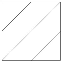
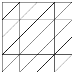
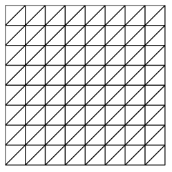
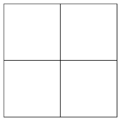
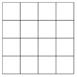
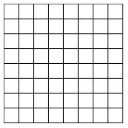
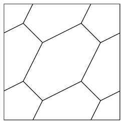
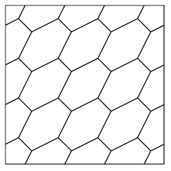
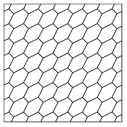
In the following computations, we employ uniform triangular grids, rectangular grids, and polygonal grids, as shown in Figures 1-3, respectively.

Refer to caption — Figure 1: The uniform triangular meshes with $n=2,~{}4,~{}8$

Example 5.1.

In this example, we consider the Biharmonic equation on the square domain $\Omega=(0,1)^{2}$ , and the exact solution is chosen as follows

\displaystyle u=x^{2}(1-x)^{2}y^{2}(1-y)^{2}.

It is clear that $u|_{\partial\Omega}=0$ and $\frac{\partial u}{\partial{\bf n}}|_{\partial\Omega}=0$ .

The errors and convergence rates for the SFWG method are listed in Tables 1-3. From the tables, we can find the convergence rates for the error $Q_{h}u-u_{h}$ in the $H^{1}$ and $L^{2}$ norms are of order $O(h^{k})$ and $O(h^{k+1})$ . The error convergence order is $O(h^{k-1})$ for $Q_{h}\varphi-\varphi_{h}$ in the $L^{2}$ norm. The numerical results are coincident with our theoretical analysis.

Table 1: Errors and convergence rates on triangular meshes in Example 5.1

$n$	$\|\!\|\!\|Q_{h}\varphi-\varphi_{h}\|\!\|\!\|$	Rate	$\|\!\|\!\|Q_{h}u-u_{h}\|\!\|\!\|$	Rate	$\left\\|Q_{h}\varphi-\varphi_{h}\right\\|$	Rate	$\left\\|Q_{h}u-u_{h}\right\\|$	Rate
	By the $P_{2}$ weak Galerkin finite element
16	$5.8675\mathrm{E}-02$	–	$7.8153\mathrm{E}-05$	–	$3.3439\mathrm{E}-04$	–	$4.1789\mathrm{E}-07$	–
32	$4.3407\mathrm{E}-02$	0.43	$1.9630\mathrm{E}-05$	1.99	$1.1637\mathrm{E}-04$	1.52	$5.0737\mathrm{E}-08$	3.04
64	$3.1476\mathrm{E}-02$	0.46	$4.9142\mathrm{E}-06$	2.00	$4.1265\mathrm{E}-05$	1.50	$6.2747\mathrm{E}-09$	3.02
128	$2.2556\mathrm{E}-02$	0.48	$1.2291\mathrm{E}-06$	2.00	$1.4663\mathrm{E}-05$	1.49	$7.8111\mathrm{E}-10$	3.01
	By the $P_{3}$ weak Galerkin finite element
16	$4.9264\mathrm{E}-03$	–	$3.2862\mathrm{E}-06$	–	$3.1500\mathrm{E}-05$	–	$9.8363\mathrm{E}-09$	–
32	$1.8548\mathrm{E}-03$	1.41	$4.1386\mathrm{E}-07$	2.99	$6.0192\mathrm{E}-06$	2.39	$5.9522\mathrm{E}-10$	4.05
64	$6.7498\mathrm{E}-04$	1.46	$5.1863\mathrm{E}-08$	3.00	$1.1038\mathrm{E}-06$	2.45	$3.6593\mathrm{E}-11$	4.02
128	$2.4189\mathrm{E}-04$	1.48	$6.4890\mathrm{E}-09$	3.00	$1.9855\mathrm{E}-07$	2.47	$2.2686\mathrm{E}-12$	4.01

Table 2: Errors and convergence rates on rectangular meshes in Example 5.1

$n$	$\|\!\|\!\|Q_{h}\varphi-\varphi_{h}\|\!\|\!\|$	Rate	$\|\!\|\!\|Q_{h}u-u_{h}\|\!\|\!\|$	Rate	$\left\\|Q_{h}\varphi-\varphi_{h}\right\\|$	Rate	$\left\\|Q_{h}u-u_{h}\right\\|$	Rate
	By the $P_{2}$ weak Galerkin finite element
16	$1.8588\mathrm{E}-01$	–	$8.8362\mathrm{E}-05$	–	$6.0219\mathrm{E}-04$	–	$3.0180E-06$	–
32	$1.4556\mathrm{E}-01$	0.35	$2.2756\mathrm{E}-05$	1.96	$2.1066\mathrm{E}-04$	1.52	$4.5616E-07$	2.73
64	$1.0805\mathrm{E}-01$	0.43	$5.7975\mathrm{E}-06$	1.97	$7.4677\mathrm{E}-05$	1.50	$6.3231E-08$	2.85
128	$7.8249\mathrm{E}-02$	0.47	$1.4653\mathrm{E}-06$	1.98	$2.6628\mathrm{E}-05$	1.49	$8.3385\mathrm{E}-09$	2.92
	By the $P_{3}$ weak Galerkin finite element
16	$1.2964\mathrm{E}-02$	–	$4.9116\mathrm{E}-06$	–	$6.9365\mathrm{E}-05$	–	$1.8319\mathrm{E}-08$	–
32	$5.2127\mathrm{E}-03$	1.31	$6.3524\mathrm{E}-07$	2.95	$1.4350\mathrm{E}-05$	2.27	$9.7185\mathrm{E}-10$	4.24
64	$1.9622\mathrm{E}-03$	1.41	$8.0882E-08$	2.97	$2.7562\mathrm{E}-06$	2.38	$5.3668\mathrm{E}-11$	4.18
128	$7.1558\mathrm{E}-04$	1.46	$1.0208\mathrm{E}-08$	2.99	$5.0843\mathrm{E}-07$	2.44	$3.1624\mathrm{E}-12$	4.08

Table 3: Errors and convergence rates on polygonal meshes in Example 5.1

$n$	$\|\!\|\!\|Q_{h}\varphi-\varphi_{h}\|\!\|\!\|$	Rate	$\|\!\|\!\|Q_{h}u-u_{h}\|\!\|\!\|$	Rate	$\left\\|Q_{h}\varphi-\varphi_{h}\right\\|$	Rate	$\left\\|Q_{h}u-u_{h}\right\\|$	Rate
	By the $P_{2}$ weak Galerkin finite element
16	$4.4235\mathrm{E}-01$	–	$1.6183\mathrm{E}-04$	–	$1.6034\mathrm{E}-03$	–	$5.6366\mathrm{E}-06$	–
32	$3.5657\mathrm{E}-01$	0.31	$4.2222\mathrm{E}-05$	1.94	$6.1355\mathrm{E}-04$	1.39	$8.7874\mathrm{E}-07$	2.68
64	$2.6774\mathrm{E}-01$	0.41	$1.0802\mathrm{E}-05$	1.97	$2.2588\mathrm{E}-04$	1.44	$1.2324\mathrm{E}-07$	2.83
128	$1.9482\mathrm{E}-01$	0.46	$2.7343\mathrm{E}-06$	1.98	$8.1581E-05$	1.47	$1.6349\mathrm{E}-08$	2.91
	By the $P_{3}$ weak Galerkin finite element
16	$9.4109\mathrm{E}-03$	–	$8.5082\mathrm{E}-06$	–	$5.6358\mathrm{E}-05$	–	$1.7179\mathrm{E}-08$	–
32	$3.6245\mathrm{E}-03$	1.38	$1.1584\mathrm{E}-06$	2.88	$1.1518\mathrm{E}-05$	2.29	$1.1435\mathrm{E}-09$	3.91
64	$1.3389\mathrm{E}-03$	1.44	$1.5123\mathrm{E}-07$	2.94	$2.1957\mathrm{E}-06$	2.39	$7.4368\mathrm{E}-11$	3.94
128	$4.8379\mathrm{E}-04$	1.47	$1.9324\mathrm{E}-08$	2.97	$4.0316\mathrm{E}-07$	2.45	$4.7472\mathrm{E}-12$	3.97

Example 5.2.

We choose the same solution area as in the above example. The exact solution is

\displaystyle u=\sin{(\pi x)}\sin{(\pi y)}.

This shows that $u|_{\partial\Omega}=0$ and $\frac{\partial u}{\partial{\bf n}}|_{\partial\Omega}\neq 0$ .

The related results are shown in Tables 4-6. From Tables 4-6, we can see the same order of convergence as Example 5.1, which coincides with the theorem.

Table 4: Errors and convergence rates on triangular meshes in Example 5.2

$n$	$\|\!\|\!\|Q_{h}\varphi-\varphi_{h}\|\!\|\!\|$	Rate	$\|\!\|\!\|Q_{h}u-u_{h}\|\!\|\!\|$	Rate	$\left\\|Q_{h}\varphi-\varphi_{h}\right\\|$	Rate	$\left\\|Q_{h}u-u_{h}\right\\|$	Rate
	By the $P_{2}$ weak Galerkin finite element
16	$9.1811E+00$	–	$7.4385\mathrm{E}-03$	–	$5.8928\mathrm{E}-02$	–	$3.4903\mathrm{E}-05$	–
32	$6.5266\mathrm{E}+00$	0.49	$1.8629\mathrm{E}-03$	2.00	$2.0861\mathrm{E}-02$	1.50	$4.1944\mathrm{E}-06$	3.06
64	$4.6215\mathrm{E}+00$	0.50	$4.6598\mathrm{E}-04$	2.00	$7.3777\mathrm{E}-03$	1.50	$5.1526\mathrm{E}-07$	3.03
128	$3.2691E+00$	0.50	$1.1652\mathrm{E}-04$	2.00	$2.6086\mathrm{E}-03$	1.50	$6.3906\mathrm{E}-08$	3.01
	By the $P_{3}$ weak Galerkin finite element
16	$2.5564\mathrm{E}-01$	–	$2.0336\mathrm{E}-04$	–	$1.6575\mathrm{E}-03$	–	$5.8062\mathrm{E}-07$	–
32	$9.0186\mathrm{E}-02$	1.50	$2.5500\mathrm{E}-05$	3.00	$2.9536\mathrm{E}-04$	2.49	$3.5466\mathrm{E}-08$	4.03
64	$3.1828\mathrm{E}-02$	1.50	$3.1915\mathrm{E}-06$	3.00	$5.2358\mathrm{E}-05$	2.50	$2.1929\mathrm{E}-09$	4.02
128	$1.1241\mathrm{E}-02$	1.50	$3.9914\mathrm{E}-07$	3.00	$9.2658\mathrm{E}-06$	2.50	$1.3635\mathrm{E}-10$	4.01

Table 5: Errors and convergence rates on rectangular meshes in Example 5.2

$n$	$\|\!\|\!\|Q_{h}\varphi-\varphi_{h}\|\!\|\!\|$	Rate	$\|\!\|\!\|Q_{h}u-u_{h}\|\!\|\!\|$	Rate	$\left\\|Q_{h}\varphi-\varphi_{h}\right\\|$	Rate	$\left\\|Q_{h}u-u_{h}\right\\|$	Rate
	By the $P_{2}$ weak Galerkin finite element
16	$9.7153\mathrm{E}+00$	–	$9.7509\mathrm{E}-03$	–	$3.9732\mathrm{E}-02$	–	$3.1204\mathrm{E}-05$	–
32	$6.9398\mathrm{E}+00$	0.49	$2.4386\mathrm{E}-03$	2.00	$1.4154\mathrm{E}-02$	1.49	$2.7188\mathrm{E}-06$	3.52
64	$4.9198\mathrm{E}+00$	0.50	$6.0947\mathrm{E}-04$	2.00	$5.0143\mathrm{E}-03$	1.50	$2.8334\mathrm{E}-07$	3.26
128	$3.4811\mathrm{E}+00$	0.50	$1.5233\mathrm{E}-04$	2.00	$1.7738\mathrm{E}-03$	1.50	$3.3224\mathrm{E}-08$	3.09
	By the $P_{3}$ weak Galerkin finite element
16	$1.5239\mathrm{E}-01$	–	$3.0553\mathrm{E}-04$	–	$5.6483\mathrm{E}-04$	–	$6.9886\mathrm{E}-07$	–
32	$5.2705\mathrm{E}-02$	1.53	$3.8294\mathrm{E}-05$	3.00	$9.5049\mathrm{E}-05$	2.57	$4.3065\mathrm{E}-08$	4.02
64	$1.8493\mathrm{E}-02$	1.51	$4.7900\mathrm{E}-06$	3.00	$1.6481\mathrm{E}-05$	2.53	$2.6808\mathrm{E}-09$	4.01
128	$6.5198\mathrm{E}-03$	1.50	$5.9886\mathrm{E}-07$	3.00	$2.8899\mathrm{E}-06$	2.51	$1.6737\mathrm{E}-10$	4.00

Table 6: Errors and convergence rates on polygonal meshes in Example 5.2

$n$	$\|\!\|\!\|Q_{h}\varphi-\varphi_{h}\|\!\|\!\|$	Rate	$\|\!\|\!\|Q_{h}u-u_{h}\|\!\|\!\|$	Rate	$\left\\|Q_{h}\varphi-\varphi_{h}\right\\|$	Rate	$\left\\|Q_{h}u-u_{h}\right\\|$	Rate
	By the $P_{2}$ weak Galerkin finite element
16	$5.1328\mathrm{E}+01$	–	$1.2790\mathrm{E}-02$	–	$2.4905\mathrm{E}-01$	–	$2.1091\mathrm{E}-04$	–
32	$3.6720\mathrm{E}+01$	0.48	$3.1524\mathrm{E}-03$	2.02	$8.8945\mathrm{E}-02$	1.49	$2.6967\mathrm{E}-05$	2.97
64	$2.6046\mathrm{E}+01$	0.50	$7.8318\mathrm{E}-04$	2.01	$3.1523\mathrm{E}-02$	1.50	$3.5157\mathrm{E}-06$	2.94
128	$1.8433\mathrm{E}+01$	0.50	$1.9526\mathrm{E}-04$	2.00	$1.1151\mathrm{E}-02$	1.50	$4.5238\mathrm{E}-07$	2.96
	By the $P_{3}$ weak Galerkin finite element
16	$6.2345\mathrm{E}-01$	–	$4.9235\mathrm{E}-04$	–	$3.9976\mathrm{E}-03$	–	$5.6491\mathrm{E}-07$	–
32	$2.2038\mathrm{E}-01$	1.50	$6.3217\mathrm{E}-05$	2.96	$7.2734\mathrm{E}-04$	2.46	$3.1102\mathrm{E}-08$	4.18
64	$7.7966\mathrm{E}-02$	1.50	$8.0051\mathrm{E}-06$	2.98	$1.3035\mathrm{E}-04$	2.48	$1.8314\mathrm{E}-09$	4.09
128	$2.7581\mathrm{E}-02$	1.50	$1.0070\mathrm{E}-06$	2.99	$2.3197\mathrm{E}-05$	2.49	$1.1132\mathrm{E}-10$	4.04

Example 5.3.

We choose the same solution area as in the above examples. The exact solution is

\displaystyle u=e^{x+y},

which satisfies $u|_{\partial\Omega}\neq 0$ and $\frac{\partial u}{\partial{\bf n}}|_{\partial\Omega}\neq 0$ .

The relevant results are displayed in Tables 7-8, which are consistent with the theoretical results.

Table 7: Errors and convergence rates on triangular meshes in Example 5.3

$n$	$\|\!\|\!\|Q_{h}\varphi-\varphi_{h}\|\!\|\!\|$	Rate	$\|\!\|\!\|Q_{h}u-u_{h}\|\!\|\!\|$	Rate	$\left\\|Q_{h}\varphi-\varphi_{h}\right\\|$	Rate	$\left\\|Q_{h}u-u_{h}\right\\|$	Rate
	By the $P_{2}$ weak Galerkin finite element
16	$2.4698\mathrm{E}+00$	–	$2.1195\mathrm{E}-03$	–	$1.6056\mathrm{E}-02$	–	$8.4842\mathrm{E}-06$	–
32	$1.7491\mathrm{E}+00$	0.50	$5.3048\mathrm{E}-04$	2.00	$5.6647\mathrm{E}-03$	1.50	$1.0618\mathrm{E}-06$	3.00
64	$1.2376\mathrm{E}+00$	0.50	$1.3269\mathrm{E}-04$	2.00	$2.0004\mathrm{E}-03$	1.50	$1.3289\mathrm{E}-07$	3.00
128	$8.7543\mathrm{E}-01$	0.50	$3.3179\mathrm{E}-05$	2.00	$7.0679\mathrm{E}-04$	1.50	$1.6623\mathrm{E}-08$	3.00
	By the $P_{3}$ weak Galerkin finite element
16	$2.5285\mathrm{E}-02$	–	$1.8753\mathrm{E}-05$	–	$1.6657\mathrm{E}-04$	–	$5.3828\mathrm{E}-08$	–
32	$8.9885\mathrm{E}-03$	1.49	$2.3491\mathrm{E}-06$	3.00	$2.9758\mathrm{E}-05$	2.48	$3.2872\mathrm{E}-09$	4.03
64	$3.1862\mathrm{E}-03$	1.50	$2.9394\mathrm{E}-07$	3.00	$5.2877\mathrm{E}-06$	2.49	$2.0294\mathrm{E}-10$	4.02
128	$1.1326\mathrm{E}-03$	1.49	$3.6753\mathrm{E}-08$	3.00	$9.4181\mathrm{E}-07$	2.49	$1.2997\mathrm{E}-11$	3.96

Table 8: Errors and convergence rates on polygonal meshes in Example 5.3

$n$	$\|\!\|\!\|Q_{h}\varphi-\varphi_{h}\|\!\|\!\|$	Rate	$\|\!\|\!\|Q_{h}u-u_{h}\|\!\|\!\|$	Rate	$\left\\|Q_{h}\varphi-\varphi_{h}\right\\|$	Rate	$\left\\|Q_{h}u-u_{h}\right\\|$	Rate
	By the $P_{2}$ weak Galerkin finite element
16	$1.2510\mathrm{E}+01$	–	$3.3152\mathrm{E}-03$	–	$6.3503\mathrm{E}-02$	–	$2.6849\mathrm{E}-05$	–
32	$9.1780\mathrm{E}+00$	0.45	$8.2523\mathrm{E}-04$	2.01	$2.3430\mathrm{E}-02$	1.44	$3.6017\mathrm{E}-06$	2.90
64	$6.6115\mathrm{E}+00$	0.47	$2.0561\mathrm{E}-04$	2.00	$8.4615\mathrm{E}-03$	1.47	$4.6959\mathrm{E}-07$	2.94
128	$4.7189\mathrm{E}+00$	0.49	$5.1299\mathrm{E}-05$	2.00	$3.0235\mathrm{E}-03$	1.48	$5.9940\mathrm{E}-08$	2.97
	By the $P_{3}$ weak Galerkin finite element
16	$5.4327\mathrm{E}-02$	–	$4.3784\mathrm{E}-05$	–	$3.5923\mathrm{E}-04$	–	$4.3622\mathrm{E}-08$	–
32	$1.9577\mathrm{E}-02$	1.47	$5.6822\mathrm{E}-06$	2.95	$6.5444\mathrm{E}-05$	2.46	$2.3973\mathrm{E}-09$	4.19
64	$6.9872\mathrm{E}-03$	1.49	$7.2357\mathrm{E}-07$	2.97	$1.1742\mathrm{E}-05$	2.48	$1.3815\mathrm{E}-10$	4.12
128	$2.4765\mathrm{E}-03$	1.50	$9.1265\mathrm{E}-08$	2.99	$2.0900\mathrm{E}-06$	2.49	$1.1196\mathrm{E}-11$	3.63

From Tables 1-8, it can be seen that under various boundary conditions, the numerical examples consistently achieve the optimal convergence order, aligning with previous theoretical analyses and affirming the accuracy of the SFWG method. Notably, the convergence order of $|\!|\!|Q_{h}\varphi-\varphi_{h}|\!|\!|$ is half order higher than the theoretical order $O(h^{k-2})$ .

6 Conclusion

In this paper, we propose a stabilizer-free weak Galerkin (SFWG) method for the Ciarlet-Raviart mixed variational form of the Biharmonic equation and analyze the well-posedness and convergence of the SFWG method. We derive the optimal error estimates about the actual variable $u$ in the $H^{1}$ and $L^{2}$ norms. Finally, we use numerical examples to verify the theoretical analysis. In future work, we will continue to study the WG related methods for the mixed form of the Biharmonic equation to reach the optimal error estimates in $H^{1}$ and $L^{2}$ norms for the auxiliary variable $\varphi$ .

Acknowledgements

This work was supported by the National Natural Science Foundation of China (grant No. 12271208, 12201246, 22341302), the National Key Research and Development Program of China (grant No. 2020YFA0713602, 2023YFA1008803), and the Key Laboratory of Symbolic Computation and Knowledge Engineering of Ministry of Education of China housed at Jilin University.

Data Availability

The code used in this work will be made available upon request to the authors.

Appendix A Some Technical Results of Ritz and Neumann Projections

Lemma A.1.

For the definitions of $\Pi_{h}^{R}$ and $\Pi_{h}^{N}$ , we have the following error equations:

	$\displaystyle(\nabla_{w}(\Pi_{h}^{R}v-v),\nabla_{w}\psi)_{{\mathcal{T}}_{h}}=$	$\displaystyle~{}l(v,\psi),\qquad\forall\,\psi\in V_{h}^{0},$		(A.1)
	$\displaystyle(\nabla_{w}(\Pi_{h}^{N}v-v),\nabla_{w}\psi)_{{\mathcal{T}}_{h}}=$	$\displaystyle~{}l(v,\psi),\qquad\forall\,\psi\in V_{h},$		(A.2)

where

l(v,\psi)=\langle({\mathbb{Q}}_{h}\nabla v-\nabla v)\cdot{\bf n},\psi_{0}-\psi_{b}\rangle_{\partial{\mathcal{T}}_{h}}.

For any $v\in H^{m+1}(\Omega),~{}(1\leq m\leq j+1)$ and for any $\psi\in V_{h}$ , we can deduce the estimate as follows

\displaystyle\big{|}l(v,\psi)\big{|}\lesssim~{}h^{m}\left\|v\right\|_{m+1}|\!|\!|\psi|\!|\!|.

(A.3)

Proof.

Using the integration by parts, the definitions of ${\mathbb{Q}}_{h}$ and $\nabla_{w}$ , (3.14), we have

$\displaystyle(-\Delta v,\psi_{0})_{{\mathcal{T}}_{h}}=$	$\displaystyle~{}(\nabla v,\nabla\psi_{0})_{{\mathcal{T}}_{h}}-\langle\nabla v\cdot{\bf n},\psi_{0}\rangle_{\partial{\mathcal{T}}_{h}}$
$\displaystyle=$	$\displaystyle~{}({\mathbb{Q}}_{h}\nabla v,\nabla\psi_{0})_{{\mathcal{T}}_{h}}-\langle\nabla v\cdot{\bf n},\psi_{0}\rangle_{\partial{\mathcal{T}}_{h}}$
$\displaystyle=$	$\displaystyle~{}-(\nabla\cdot{\mathbb{Q}}_{h}\nabla v,\psi_{0})_{{\mathcal{T}}_{h}}+\langle({\mathbb{Q}}_{h}\nabla v-\nabla v)\cdot{\bf n},\psi_{0}\rangle_{\partial{\mathcal{T}}_{h}}$
$\displaystyle=$	$\displaystyle~{}({\mathbb{Q}}_{h}\nabla v,\nabla_{w}\psi)-\langle{\mathbb{Q}}_{h}\nabla v\cdot{\bf n},\psi_{b}\rangle_{\partial{\mathcal{T}}_{h}}+\langle({\mathbb{Q}}_{h}\nabla v-\nabla v)\cdot{\bf n},\psi_{0}\rangle_{\partial{\mathcal{T}}_{h}}$
$\displaystyle=$	$\displaystyle~{}(\nabla_{w}v,\nabla_{w}\psi)_{{\mathcal{T}}_{h}}-\langle({\mathbb{Q}}_{h}\nabla v-\nabla v)\cdot{\bf n},\psi_{b}\rangle_{\partial{\mathcal{T}}_{h}}-\langle\nabla v\cdot{\bf n},\psi_{b}\rangle_{\partial{\mathcal{T}}_{h}}$
	$\displaystyle~{}+\langle({\mathbb{Q}}_{h}\nabla v-\nabla v)\cdot{\bf n},\psi_{0}\rangle_{\partial{\mathcal{T}}_{h}}$
$\displaystyle=$	$\displaystyle~{}(\nabla_{w}v,\nabla_{w}\psi)_{{\mathcal{T}}_{h}}+\langle({\mathbb{Q}}_{h}\nabla v-\nabla v)\cdot{\bf n},\psi_{0}-\psi_{b}\rangle_{\partial{\mathcal{T}}_{h}}-\langle\nabla v\cdot{\bf n},\psi_{b}\rangle_{\partial{\mathcal{T}}_{h}}.$	(A.4)

By the above equation and the fact that $\psi|_{\partial\Omega}=0$ and (4.1), we arrive at (A.1). Using (4.2), we get (A.2).

For (A.3), we use the Cauchy-Schwarz inequality, the trace inequality, the projection inequality, the definition of $\left\|\cdot\right\|_{1,h}$ , (3.1), and get

	$\displaystyle\big{\|}l(v,\psi)\big{\|}=$	$\displaystyle~{}\Big{\|}\langle({\mathbb{Q}}_{h}\nabla v-\nabla v)\cdot{\bf n},\psi_{0}-\psi_{b}\rangle_{\partial{\mathcal{T}}_{h}}\Big{\|}$
	$\displaystyle\lesssim$	$\displaystyle~{}\left(\sum_{T\in\mathcal{T}_{h}}h_{T}\left\\|{\mathbb{Q}}_{h}\nabla v-\nabla v\right\\|_{\partial T}^{2}\right)^{\frac{1}{2}}\left(\sum_{T\in\mathcal{T}_{h}}h_{T}^{-1}\left\\|\psi_{0}-\psi_{b}\right\\|_{\partial T}^{2}\right)^{\frac{1}{2}}$
	$\displaystyle\lesssim$	$\displaystyle~{}h^{m}\left\\|\nabla v\right\\|_{m}\left\\|\psi\right\\|_{1,h}$
	$\displaystyle\lesssim$	$\displaystyle~{}h^{m}\left\\|v\right\\|_{m+1}\|\!\|\!\|\psi\|\!\|\!\|.$

Then we completes the proof. ∎

Lemma A.2.

For any $v\in H^{m+1}(\Omega),(0\leq m\leq k)$ , there holds

\displaystyle|\!|\!|v-Q_{h}v|\!|\!|\lesssim h^{m}\left\|v\right\|_{m+1}.

(A.5)

Proof.

We use the definition of the weak gradient, the integration by parts, the Cauchy-Schwarz inequality, the trace inequality, the inverse inequality, the definition of the projection operator, and the projection inequality to obtain for any ${\mathbf{q}}\in[P_{j}(T)]^{d}$ ,

	$\displaystyle~{}(\nabla_{w}(v-Q_{h}v),{\mathbf{q}})_{T}$
	$\displaystyle~{}=-(v-Q_{0}v,\nabla\cdot{\mathbf{q}})_{T}+\langle v-Q_{b}v,{\mathbf{q}}\cdot{\bf n}\rangle_{\partial T}$
	$\displaystyle~{}=(\nabla(v-Q_{0}v),{\mathbf{q}})_{T}-\langle v-Q_{0}v-(v-Q_{b}v),{\mathbf{q}}\cdot{\bf n}\rangle_{\partial T}$
	$\displaystyle~{}\lesssim\left\\|\nabla(v-Q_{0}v)\right\\|\left\\|{\mathbf{q}}\right\\|+\left(\sum_{T\in\mathcal{T}_{h}}h_{T}^{-1}\left\\|Q_{0}v-Q_{b}v\right\\|_{\partial T}^{2}\right)^{\frac{1}{2}}\left(\sum_{T\in\mathcal{T}_{h}}h_{T}\left\\|{\mathbf{q}}\cdot{\bf n}\right\\|_{\partial T}^{2}\right)^{\frac{1}{2}}$
	$\displaystyle~{}\lesssim\left\\|\nabla(v-Q_{0}v)\right\\|\left\\|{\mathbf{q}}\right\\|+\left(\sum_{T\in\mathcal{T}_{h}}h_{T}^{-1}(\left\\|v-Q_{0}v\right\\|_{\partial T}^{2}+\left\\|v-Q_{b}v\right\\|_{\partial T}^{2})\right)^{\frac{1}{2}}\left\\|{\mathbf{q}}\right\\|$
	$\displaystyle~{}\lesssim\left\\|\nabla(v-Q_{0}v)\right\\|\left\\|{\mathbf{q}}\right\\|+\left(\sum_{T\in\mathcal{T}_{h}}h_{T}^{-1}\left\\|v-Q_{0}v\right\\|_{\partial T}^{2}\right)^{\frac{1}{2}}\left\\|{\mathbf{q}}\right\\|$
	$\displaystyle~{}\lesssim\left\\|\nabla(v-Q_{0}v)\right\\|\left\\|{\mathbf{q}}\right\\|+\left(\sum_{T\in\mathcal{T}_{h}}h_{T}^{-2}\left\\|v-Q_{0}v\right\\|_{T}^{2}+\left\\|\nabla(v-Q_{0}v)\right\\|_{T}^{2}\right)^{\frac{1}{2}}\left\\|{\mathbf{q}}\right\\|$
	$\displaystyle~{}\lesssim h^{m}\left\\|v\right\\|_{m+1}\left\\|{\mathbf{q}}\right\\|.$

Let ${\mathbf{q}}=\nabla_{w}(v-Q_{h}v)$ , then we get (A.5). ∎

Lemma A.3.

For $v\in H^{1}_{0}(\Omega)\bigcap H^{m+1}(\Omega)$ or $\overline{H}^{1}(\Omega)\bigcap H^{m+1}(\Omega)$ , where $1\leq m\leq k$ , we have

	$\displaystyle\|\!\|\!\|v-\Pi_{h}^{R}v\|\!\|\!\|\lesssim$	$\displaystyle~{}h^{m}\left\\|v\right\\|_{m+1},$		(A.6)
	$\displaystyle\|\!\|\!\|v-\Pi_{h}^{N}v\|\!\|\!\|\lesssim$	$\displaystyle~{}h^{m}\left\\|v\right\\|_{m+1}.$		(A.7)

Proof.

For (A.6), by using (A.1), the estimate of $l(v,\psi)$ and the Young’s inequality, we get

	$\displaystyle\|\!\|\!\|v-\Pi_{h}^{R}v\|\!\|\!\|^{2}=$	$\displaystyle~{}(\nabla_{w}(v-\Pi_{h}^{R}v),\nabla_{w}(v-Q_{h}v))_{{\mathcal{T}}_{h}}+(\nabla_{w}(v-\Pi_{h}^{R}v),\nabla_{w}(Q_{h}v-\Pi_{h}^{R}v))_{{\mathcal{T}}_{h}}$
	$\displaystyle\lesssim$	$\displaystyle~{}\|\!\|\!\|v-Q_{h}v\|\!\|\!\|\|\!\|\!\|v-\Pi_{h}^{R}v\|\!\|\!\|+\big{\|}l(v,Q_{h}v-\Pi_{h}^{R}v)\big{\|}$
	$\displaystyle\lesssim$	$\displaystyle~{}\|\!\|\!\|v-Q_{h}v\|\!\|\!\|\|\!\|\!\|v-\Pi_{h}^{R}v\|\!\|\!\|+h^{m}\left\\|v\right\\|_{m+1}\|\!\|\!\|Q_{h}v-\Pi_{h}^{R}v\|\!\|\!\|$
	$\displaystyle\lesssim$	$\displaystyle~{}\|\!\|\!\|v-Q_{h}v\|\!\|\!\|\|\!\|\!\|v-\Pi_{h}^{R}v\|\!\|\!\|+h^{m}\left\\|v\right\\|_{m+1}(\|\!\|\!\|Q_{h}v-v\|\!\|\!\|+\|\!\|\!\|v-\Pi_{h}^{R}v\|\!\|\!\|)$
	$\displaystyle\leq$	$\displaystyle~{}Ch^{2m}\left\\|v\right\\|_{m+1}^{2}+\frac{1}{2}\|\!\|\!\|v-\Pi_{h}^{R}v\|\!\|\!\|^{2}.$

Thus, we have (A.6). Analogously, we use (A.2) and same inequalities to verify (A.7). ∎

Corollary A.1.

For $v\in H^{1}_{0}(\Omega)\bigcap H^{m+1}(\Omega)$ or $\overline{H}^{1}(\Omega)\bigcap H^{m+1}(\Omega)$ , where $1\leq m\leq k$ , there hold

	$\displaystyle\left\\|v-\Pi_{h}^{R}v\right\\|_{1,h}\lesssim$	$\displaystyle~{}h^{m}\left\\|v\right\\|_{m+1},$		(A.8)
	$\displaystyle\left\\|v-\Pi_{h}^{N}v\right\\|_{1,h}\lesssim$	$\displaystyle~{}h^{m}\left\\|v\right\\|_{m+1}.$		(A.9)

Proof.

Using Lemma 3.1, the definitions of $\left\|\cdot\right\|_{1,h}$ and $Q_{b}$ , the trace inequality, the projection inequality, Lemma A.2 and Lemma A.3, we have

		$\displaystyle~{}\left\\|v-\Pi_{h}^{R}v\right\\|_{1,h}$
	$\displaystyle\lesssim$	$\displaystyle~{}\left\\|v-Q_{h}v\right\\|_{1,h}+\left\\|Q_{h}v-\Pi_{h}^{R}v\right\\|_{1,h}$
	$\displaystyle\lesssim$	$\displaystyle~{}\left(\sum_{T\in\mathcal{T}_{h}}\left\\|\nabla(v-Q_{0}v)\right\\|_{T}^{2}+h^{-1}\left\\|v-Q_{0}v-(v-Q_{b}v)\right\\|_{\partial T}^{2}\right)^{\frac{1}{2}}+\|\!\|\!\|Q_{h}v-\Pi_{h}^{R}v\|\!\|\!\|$
	$\displaystyle\lesssim$	$\displaystyle~{}\left(\sum_{T\in\mathcal{T}_{h}}\left\\|\nabla(v-Q_{0}v)\right\\|_{T}^{2}+h^{-1}\left\\|v-Q_{0}v-(v-Q_{b}v)\right\\|_{\partial T}^{2}\right)^{\frac{1}{2}}+\|\!\|\!\|Q_{h}v-v\|\!\|\!\|+\|\!\|\!\|v-\Pi_{h}^{R}v\|\!\|\!\|$
	$\displaystyle\lesssim$	$\displaystyle~{}\left(\sum_{T\in\mathcal{T}_{h}}\left\\|\nabla(v-Q_{0}v)\right\\|_{T}^{2}+h^{-1}\left\\|v-Q_{0}v\right\\|_{\partial T}^{2}\right)^{\frac{1}{2}}+h^{m}\left\\|v\right\\|_{m+1}$
	$\displaystyle\lesssim$	$\displaystyle~{}h^{m}\left\\|v\right\\|_{m+1},$

which completes the proof of (A.8). The (A.9) can be verified in the similar way. ∎

Lemma A.4.

For $v\in H^{1}_{0}(\Omega)\bigcap H^{m+1}(\Omega)$ or $\overline{H}^{1}(\Omega)\bigcap H^{m+1}(\Omega)$ , where $1\leq m\leq k$ , we have

	$\displaystyle\left\\|Q_{0}v-\Pi_{0}^{R}v\right\\|\lesssim$	$\displaystyle~{}h^{m+1}\left\\|v\right\\|_{m+1}$		(A.10)
	$\displaystyle\left\\|Q_{0}v-\Pi_{0}^{N}v\right\\|\lesssim$	$\displaystyle~{}h^{m+1}\left\\|v\right\\|_{m+1}.$		(A.11)

Further, we arrive at

	$\displaystyle\left\\|v-\Pi_{0}^{R}v\right\\|\lesssim$	$\displaystyle~{}h^{m+1}\left\\|v\right\\|_{m+1}$		(A.12)
	$\displaystyle\left\\|v-\Pi_{0}^{N}v\right\\|\lesssim$	$\displaystyle~{}h^{m+1}\left\\|v\right\\|_{m+1}.$		(A.13)

Proof.

First, we use the standard duality argument to prove (A.11) and (A.13) in detail. Find $\phi\in\overline{H}^{1}(\Omega)$ such that

	$\displaystyle-\Delta\phi=$	$\displaystyle~{}Q_{0}v-\Pi_{0}^{N}v,\quad in~{}\Omega,$		(A.14)
	$\displaystyle\frac{\partial\phi}{\partial{\bf n}}=$	$\displaystyle~{}0,\quad\qquad\qquad\,\,\,on~{}\partial\Omega,$		(A.15)

and the above dual problem has the regularity assumption

\left\|\phi\right\|_{2}\lesssim\left\|Q_{0}v-\Pi_{0}^{N}v\right\|.

By (A.4), (A.15), the Cauchy-Schwarz inequality, the projection inequality, (A.7), (A.2), and (A.3), we get

		$\displaystyle\left\\|Q_{0}v-\Pi_{0}^{N}v\right\\|^{2}$
	$\displaystyle=$	$\displaystyle~{}(-\Delta\phi,Q_{0}v-\Pi_{0}^{N}v)_{{\mathcal{T}}_{h}}$
	$\displaystyle=$	$\displaystyle~{}(\nabla_{w}\phi,\nabla_{w}(Q_{h}v-\Pi_{h}^{N}v))_{{\mathcal{T}}_{h}}+l(\phi,Q_{h}v-\Pi_{h}^{N}v)$
	$\displaystyle=$	$\displaystyle~{}(\nabla_{w}(\phi-\Pi_{h}^{N}\phi),\nabla_{w}(Q_{h}v-\Pi_{h}^{N}v))_{{\mathcal{T}}_{h}}+(\nabla_{w}\Pi_{h}^{N}\phi,\nabla_{w}(Q_{h}v-\Pi_{h}^{N}v))_{{\mathcal{T}}_{h}}$
		$\displaystyle~{}+l(\phi,Q_{h}v-\Pi_{h}^{N}v)$
	$\displaystyle\lesssim$	$\displaystyle~{}\|\!\|\!\|\phi-\Pi_{h}^{N}\phi\|\!\|\!\|(\|\!\|\!\|Q_{h}v-v\|\!\|\!\|+\|\!\|\!\|v-\Pi_{h}^{N}v\|\!\|\!\|)+(\nabla_{w}\Pi_{h}^{N}\phi,\nabla_{w}(Q_{h}v-v))_{{\mathcal{T}}_{h}}$
		$\displaystyle~{}+(\nabla_{w}\Pi_{h}^{N}\phi,\nabla_{w}(v-\Pi_{h}^{N}v))_{{\mathcal{T}}_{h}}+l(\phi,Q_{h}v-\Pi_{h}^{N}v)$
	$\displaystyle\lesssim$	$\displaystyle~{}h\left\\|\phi\right\\|_{2}h^{m}\left\\|v\right\\|_{m+1}+(\nabla_{w}(\Pi_{h}^{N}\phi-\phi),\nabla_{w}(Q_{h}v-v))_{{\mathcal{T}}_{h}}+(\nabla_{w}\phi,\nabla_{w}(Q_{h}v-v))_{{\mathcal{T}}_{h}}$
		$\displaystyle~{}-l(v,\Pi_{h}^{N}\phi)+l(\phi,Q_{h}v-\Pi_{h}^{N}v)$
	$\displaystyle\lesssim$	$\displaystyle~{}h^{m+1}\left\\|v\right\\|_{m+1}\left\\|\phi\right\\|_{2}+h\left\\|\phi\right\\|_{2}h^{m}\left\\|v\right\\|_{m+1}+(\nabla_{w}\phi,\nabla_{w}(Q_{h}v-v))_{{\mathcal{T}}_{h}}-l(v,\Pi_{h}^{N}\phi)$
		$\displaystyle~{}+l(\phi,Q_{h}v-\Pi_{h}^{N}v)$
	$\displaystyle\lesssim$	$\displaystyle~{}h^{m+1}\left\\|v\right\\|_{m+1}\left\\|\phi\right\\|_{2}+(\nabla_{w}\phi,\nabla_{w}(Q_{h}v-v))_{{\mathcal{T}}_{h}}-l(v,\Pi_{h}^{N}\phi)$
		$\displaystyle~{}+h\left\\|\phi\right\\|_{2}(\|\!\|\!\|Q_{h}v-v\|\!\|\!\|+\|\!\|\!\|v-\Pi_{h}^{N}v\|\!\|\!\|)$
	$\displaystyle\lesssim$	$\displaystyle~{}h^{m+1}\left\\|v\right\\|_{m+1}\left\\|\phi\right\\|_{2}+(\nabla_{w}\phi,\nabla_{w}(Q_{h}v-v))_{{\mathcal{T}}_{h}}-l(v,\Pi_{h}^{N}\phi).$

For $(\nabla_{w}\phi,\nabla_{w}(Q_{h}v-v))_{{\mathcal{T}}_{h}}$ , by using (3.14), the definitions of the projection operator and the weak gradient $\nabla_{w}$ , (A.14), (A.15), the Cauchy-Schwarz inequality, and the projection inequality, we have

	$\displaystyle(\nabla_{w}\phi,\nabla_{w}(Q_{h}v-v))_{{\mathcal{T}}_{h}}=$	$\displaystyle~{}({\mathbb{Q}}_{h}\nabla\phi,\nabla_{w}(Q_{h}v-v))_{{\mathcal{T}}_{h}}$
	$\displaystyle=$	$\displaystyle~{}(\nabla\phi,\nabla_{w}(Q_{h}v-v))_{{\mathcal{T}}_{h}}$
	$\displaystyle=$	$\displaystyle~{}-(Q_{0}v-v,\nabla\cdot\nabla\phi)_{{\mathcal{T}}_{h}}+\langle Q_{b}v-v,\nabla\phi\cdot{\bf n}\rangle_{\partial{\mathcal{T}}_{h}}$
	$\displaystyle=$	$\displaystyle~{}(Q_{0}v-v,Q_{0}v-\Pi_{0}^{N}v)_{{\mathcal{T}}_{h}}$
	$\displaystyle=$	$\displaystyle~{}\left\\|Q_{0}v-v\right\\|\left\\|Q_{0}v-\Pi_{0}^{N}v\right\\|$
	$\displaystyle\lesssim$	$\displaystyle~{}h^{m+1}\left\\|v\right\\|_{m+1}\left\\|Q_{0}v-\Pi_{0}^{N}v\right\\|$

As to $l(v,\Pi_{h}^{N}\phi)$ , we have

	$\displaystyle l(v,\Pi_{h}^{N}\phi)=$	$\displaystyle~{}\langle({\mathbb{Q}}_{h}\nabla v-\nabla v)\cdot{\bf n},\Pi_{0}^{N}\phi-\Pi_{b}^{N}\phi\rangle_{\partial{\mathcal{T}}_{h}}$
	$\displaystyle\leq$	$\displaystyle~{}\Big{(}\sum_{T\in\mathcal{T}_{h}}h_{T}\left\\|{\mathbb{Q}}_{h}\nabla v-\nabla v\right\\|_{\partial T}^{2}\Big{)}^{\frac{1}{2}}\Big{(}\sum_{T\in\mathcal{T}_{h}}h_{T}^{-1}\left\\|\Pi_{0}^{N}\phi-\Pi_{b}^{N}\phi\right\\|_{\partial T}^{2}\Big{)}^{\frac{1}{2}}$
	$\displaystyle\lesssim$	$\displaystyle~{}\Big{(}\sum_{T\in\mathcal{T}_{h}}\left\\|{\mathbb{Q}}_{h}\nabla v-\nabla v\right\\|_{T}^{2}+h_{T}^{2}\left\\|\nabla({\mathbb{Q}}_{h}\nabla v-\nabla v)\right\\|_{T}^{2}\Big{)}^{\frac{1}{2}}$
		$\displaystyle~{}\Big{(}\sum_{T\in\mathcal{T}_{h}}h_{T}^{-1}\left\\|\Pi_{0}^{N}\phi-\phi-(\Pi_{b}^{N}\phi-\phi)\right\\|_{\partial T}^{2}\Big{)}^{\frac{1}{2}}$
	$\displaystyle\lesssim$	$\displaystyle~{}h^{m}\left\\|v\right\\|_{m+1}\left\\|\Pi_{h}^{N}\phi-\phi\right\\|_{1,h}$
	$\displaystyle\lesssim$	$\displaystyle~{}h^{m+1}\left\\|v\right\\|_{m+1}\left\\|\phi\right\\|_{2},$

where we have utilized the Cauchy-Schwarz inequality, the trace inequality, the projection inequality and (A.9). Thus, we get

	$\displaystyle\left\\|Q_{0}v-\Pi_{0}^{N}v\right\\|^{2}\lesssim$	$\displaystyle~{}h^{m+1}\left\\|v\right\\|_{m+1}\left\\|\phi\right\\|_{2}+h^{m+1}\left\\|v\right\\|_{m+1}\left\\|Q_{0}v-\Pi_{0}^{N}v\right\\|$
	$\displaystyle\lesssim$	$\displaystyle~{}h^{m+1}\left\\|v\right\\|_{m+1}\left\\|Q_{0}v-\Pi_{0}^{N}v\right\\|+h^{m+1}\left\\|v\right\\|_{m+1}\left\\|Q_{0}v-\Pi_{0}^{N}v\right\\|$
	$\displaystyle\lesssim$	$\displaystyle~{}h^{m+1}\left\\|v\right\\|_{m+1}\left\\|Q_{0}v-\Pi_{0}^{N}v\right\\|,$

which implies

\left\|Q_{0}v-\Pi_{0}^{N}v\right\|\lesssim h^{m+1}\left\|v\right\|_{m+1}.

Furthermore, we have

	$\displaystyle\left\\|v-\Pi_{0}^{N}v\right\\|\leq$	$\displaystyle~{}\left\\|v-Q_{0}v\right\\|+\left\\|Q_{0}v-\Pi_{0}^{N}v\right\\|$
	$\displaystyle\lesssim$	$\displaystyle~{}h^{m+1}\left\\|v\right\\|_{m+1}+h^{m+1}\left\\|v\right\\|_{m+1}$
	$\displaystyle\lesssim$	$\displaystyle~{}h^{m+1}\left\\|v\right\\|_{m+1},$

which completes the proof of (A.11) and (A.13).

To verify the estimate (A.12), we consider the dual problem as follows

	$\displaystyle-\Delta\phi=$	$\displaystyle~{}Q_{0}v-\Pi_{0}^{R}v,\quad in~{}\Omega,$		(A.16)
	$\displaystyle\phi=$	$\displaystyle~{}0,\quad\qquad\qquad\,\,on~{}\partial\Omega.$		(A.17)

Using the above problem, $Q_{h}v-\Pi_{h}^{R}v\in V_{h}^{0}$ and $v|_{\partial\Omega}=0$ , we can obtain the same derivation process and results. The proof is completed. ∎

Corollary A.2.

For $v\in H^{1}_{0}(\Omega)\bigcap H^{m+1}(\Omega)$ or $\overline{H}^{1}(\Omega)\bigcap H^{m+1}(\Omega)$ , where $1\leq m\leq k$ , we have

	$\displaystyle\left\\|Q_{h}v-\Pi_{h}^{R}v\right\\|_{0,h}\lesssim$	$\displaystyle~{}h^{m+1}\left\\|v\right\\|_{m+1},$		(A.18)
	$\displaystyle\left\\|Q_{h}v-\Pi_{h}^{N}v\right\\|_{0,h}\lesssim$	$\displaystyle~{}h^{m+1}\left\\|v\right\\|_{m+1},$		(A.19)

Furthermore, we acquire

	$\displaystyle\left\\|v-\Pi_{h}^{R}v\right\\|_{0,h}\lesssim$	$\displaystyle~{}h^{m+1}\left\\|v\right\\|_{m+1},$		(A.20)
	$\displaystyle\left\\|v-\Pi_{h}^{N}v\right\\|_{0,h}\lesssim$	$\displaystyle~{}h^{m+1}\left\\|v\right\\|_{m+1},$		(A.21)

Proof.

By the definition of the norm $\left\|\cdot\right\|_{0,h}$ , (A.10), Lemma 3.1, (A.5) and (A.6), we have

		$\displaystyle~{}\left\\|Q_{h}v-\Pi_{h}^{R}v\right\\|_{0,h}^{2}$
	$\displaystyle=$	$\displaystyle~{}\sum_{T\in\mathcal{T}_{h}}\left\\|Q_{0}v-\Pi_{0}^{R}v\right\\|_{T}^{2}+\sum_{T\in\mathcal{T}_{h}}h\left\\|Q_{0}v-\Pi_{0}^{R}v-(Q_{b}v-\Pi_{b}^{R}v)\right\\|_{\partial T}^{2}$
	$\displaystyle\lesssim$	$\displaystyle~{}h^{2(m+1)}\left\\|v\right\\|_{m+1}^{2}+h^{2}\sum_{T\in\mathcal{T}_{h}}h^{-1}\left\\|Q_{0}v-\Pi_{0}^{R}v-(Q_{b}v-\Pi_{b}^{R}v)\right\\|_{\partial T}^{2}$
	$\displaystyle\lesssim$	$\displaystyle~{}h^{2(m+1)}\left\\|v\right\\|_{m+1}^{2}+h^{2}\left\\|Q_{h}v-\Pi_{h}^{R}v\right\\|_{1,h}^{2}$
	$\displaystyle\lesssim$	$\displaystyle~{}h^{2(m+1)}\left\\|v\right\\|_{m+1}^{2}+h^{2}\|\!\|\!\|Q_{h}v-\Pi_{h}^{R}v\|\!\|\!\|^{2}$
	$\displaystyle\lesssim$	$\displaystyle~{}h^{2(m+1)}\left\\|v\right\\|_{m+1}^{2}+h^{2}(\|\!\|\!\|Q_{h}v-v\|\!\|\!\|+\|\!\|\!\|v-\Pi_{h}^{R}v\|\!\|\!\|)^{2}$
	$\displaystyle\lesssim$	$\displaystyle~{}h^{2(m+1)}\left\\|v\right\\|_{m+1}^{2}+h^{2m+2}\left\\|v\right\\|_{m+1}^{2}$
	$\displaystyle\lesssim$	$\displaystyle~{}h^{2(m+1)}\left\\|v\right\\|_{m+1}^{2}.$

Using the definitions of $\left\|\cdot\right\|_{0,h}$ and the projection $Q_{b}$ , the trace inequality, and the projection inequality, we obtain

		$\displaystyle~{}\left\\|v-\Pi_{h}^{R}v\right\\|_{0,h}^{2}$
	$\displaystyle\lesssim$	$\displaystyle~{}\left\\|v-Q_{h}v\right\\|_{0,h}^{2}+\left\\|Q_{h}v-\Pi_{h}^{R}v\right\\|_{0,h}^{2}$
	$\displaystyle\lesssim$	$\displaystyle~{}\sum_{T\in\mathcal{T}_{h}}\left\\|v-Q_{0}v\right\\|_{T}^{2}+\sum_{T\in\mathcal{T}_{h}}h\left\\|v-Q_{0}v-(v-Q_{b}v)\right\\|_{\partial T}^{2}+h^{2(m+1)}\left\\|v\right\\|_{m+1}^{2}$
	$\displaystyle\lesssim$	$\displaystyle~{}\sum_{T\in\mathcal{T}_{h}}\left\\|v-Q_{0}v\right\\|_{T}^{2}+\sum_{T\in\mathcal{T}_{h}}h\left\\|v-Q_{0}v\right\\|_{\partial T}^{2}+h^{2(m+1)}\left\\|v\right\\|_{m+1}^{2}$
	$\displaystyle\lesssim$	$\displaystyle~{}\sum_{T\in\mathcal{T}_{h}}\left\\|v-Q_{0}v\right\\|_{T}^{2}+\sum_{T\in\mathcal{T}_{h}}h^{2}\left\\|\nabla(v-Q_{0}v)\right\\|_{T}^{2}+h^{2(m+1)}\left\\|v\right\\|_{m+1}^{2}$
	$\displaystyle\lesssim$	$\displaystyle~{}h^{2(m+1)}\left\\|v\right\\|_{m+1}^{2}.$

We complete the proof of (A.18) and (A.20). Analogously, we get (A.19) and (A.21). ∎

References

[1] D. N. Arnold, L. R. Scott, and M. Vogelius, Regular inversion of the divergence operator with Dirichlet boundary conditions on a polygon, Ann. Scuola Norm. Sup. Pisa Cl. Sci. (4), 15 (1988), pp. 169–192.
[2] F. Brezzi, Sur la méthode des éléments finis hybrides pour le problème biharmonique, Numer. Math., 24 (1975), pp. 103–131.
[3] Y. Feng, Y. Liu, R. Wang, and S. Zhang, A stabilizer-free weak Galerkin finite element method for the Stokes equations, Adv. Appl. Math. Mech., 14 (2022), pp. 181–201.
[4] L. Gastaldi and R. H. Nochetto, Sharp maximum norm error estimates for general mixed finite element approximations to second order elliptic equations, RAIRO Modél. Math. Anal. Numér., 23 (1989), pp. 103–128.
[5] J. Hu, Y. Huang, and S. Zhang, The lowest order differentiable finite element on rectangular grids, SIAM J. Numer. Anal., 49 (2011), pp. 1350–1368.
[6] C. Johnson, On the convergence of a mixed finite-element method for plate bending problems, Numer. Math., 21 (1973), pp. 43–62.
[7] T. Miyoshi, A finite element method for the solutions of fourth order partial differential equations, Kumamoto J. Sci. (Math.), 9 (1972/73), pp. 87–116.
[8] P. Monk, A mixed finite element method for the biharmonic equation, SIAM Journal on Numerical Analysis, 24 (1987), pp. 737–749.
[9] L. S. D. Morley*, The triangular equilibrium element in the solution of plate bending problems, The Aeronautical Quarterly, (1968), pp. 149–169.
[10] I. Mozolevski, E. Süli, and P. R. Bösing, $hp$ -version a priori error analysis of interior penalty discontinuous Galerkin finite element approximations to the biharmonic equation, J. Sci. Comput., 30 (2007), pp. 465–491.
[11] L. Mu, J. Wang, Y. Wang, and X. Ye, A weak Galerkin mixed finite element method for biharmonic equations, in Numerical solution of partial differential equations: theory, algorithms, and their applications, vol. 45 of Springer Proc. Math. Stat., Springer, New York, 2013, pp. 247–277.
[12] L. Mu, J. Wang, and X. Ye, A stable numerical algorithm for the Brinkman equations by weak Galerkin finite element methods, J. Comput. Phys., 273 (2014), pp. 327–342.
[13] L. Mu, J. Wang, and X. Ye, Weak Galerkin finite element methods for the biharmonic equation on polytopal meshes, Numer. Methods Partial Differential Equations, 30 (2014), pp. 1003–1029.
[14] J. T. Oden, Generalized conjugate functions for mixed finite element approximations of boundary value problems, in The mathematical foundations of the finite element method with applications to partial differential equations (Proc. Sympos., Univ. Maryland, Baltimore, Md., 1972), Academic Press, New York-London, 1972, pp. 626–669.
[15] P. Oswald, Hierarchical conforming finite element methods for the biharmonic equation, SIAM J. Numer. Anal., 29 (1992), pp. 1610–1625.
[16] P. C. RAVIART, A mixed finite element method for the biharmonic equation, Mathematical Aspects of Finite Elements in Partial Differential Equations, (1974), pp. 125–145.
[17] J. Wang, Asymptotic expansions and $L^{\infty}$ -error estimates for mixed finite element methods for second order elliptic problems, Numer. Math., 55 (1989), pp. 401–430.
[18] J. Wang and X. Ye, A weak galerkin mixed finite element method for second order elliptic problems, 83, pp. 2101–2126.
[19] J. Wang and X. Ye, A weak galerkin finite element method for second-order elliptic problems, Journal of Computational and Applied Mathematics, 241 (2013), pp. 103–115.
[20] J. Wang and X. Ye, A weak Galerkin finite element method for the stokes equations, Adv. Comput. Math., 42 (2016), pp. 155–174.
[21] X. Ye and S. Zhang, A stabilizer-free weak Galerkin finite element method on polytopal meshes, J. Comput. Appl. Math., 371 (2020), pp. 112699, 9.
[22] X. Ye and S. Zhang, A stabilizer free weak Galerkin method for the biharmonic equation on polytopal meshes, SIAM J. Numer. Anal., 58 (2020), pp. 2572–2588.
[23] R. Zhang and Q. Zhai, A weak Galerkin finite element scheme for the biharmonic equations by using polynomials of reduced order, J. Sci. Comput., 64 (2015), pp. 559–585.
[24] S. Zhang, A $C_{1}$ - $P_{2}$ finite element without nodal basis, M2AN Math. Model. Numer. Anal., 42 (2008), pp. 175–192.
[25] P. Zhu, S. Xie, and X. Wang, A stabilizer-free $C^{0}$ weak Galerkin method for the biharmonic equations, Sci. China Math., 66 (2023), pp. 627–646.

	$\displaystyle\\|v\\|^{2}_{0,h}=$	$\displaystyle~{}a(v,v)=(v_{0},v_{0})_{{\mathcal{T}}_{h}}+\sum_{T\in\mathcal{T}_{h}}h_{T}\langle v_{0}-v_{b},v_{0}-v_{b}\rangle_{\partial T},$
	$\displaystyle\|\!\|\!\|v\|\!\|\!\|^{2}=$	$\displaystyle~{}b(v,v)=(\nabla_{w}v,\nabla_{w}v)_{{\mathcal{T}}_{h}},$
	$\displaystyle\\|v\\|^{2}_{1,h}=$	$\displaystyle~{}\sum_{T\in\mathcal{T}_{h}}\left\\|\nabla v_{0}\right\\|^{2}_{T}+\sum_{T\in\mathcal{T}_{h}}h_{T}^{-1}\left\\|v_{0}-v_{b}\right\\|^{2}_{\partial T}.$

	$\displaystyle\left\\|v\right\\|_{1,h}\lesssim$	$\displaystyle~{}h^{-1}\left\\|v\right\\|_{0,h},$		(3.2)
	$\displaystyle\|\!\|\!\|v\|\!\|\!\|\lesssim$	$\displaystyle~{}h^{-1}\left\\|v\right\\|_{0,h}.$		(3.3)

	$\displaystyle\left\\|v\right\\|_{1,h}^{2}=$	$\displaystyle~{}\sum_{T\in\mathcal{T}_{h}}(\left\\|\nabla v_{0}\right\\|_{T}^{2}+h^{-1}_{T}\left\\|v_{0}-v_{b}\right\\|_{\partial T}^{2})$
	$\displaystyle\lesssim$	$\displaystyle~{}\sum_{T\in\mathcal{T}_{h}}(h^{-2}_{T}\left\\|v_{0}\right\\|_{T}^{2}+h^{-1}_{T}\left\\|v_{0}-v_{b}\right\\|_{\partial T}^{2})$
	$\displaystyle\lesssim$	$\displaystyle~{}h^{-2}\sum_{T\in\mathcal{T}_{h}}(\left\\|v_{0}\right\\|_{T}^{2}+h_{T}\left\\|v_{0}-v_{b}\right\\|_{\partial T}^{2})$
	$\displaystyle\lesssim$	$\displaystyle~{}h^{-2}\left\\|v\right\\|_{0,h}^{2},$

	$\displaystyle\left\\|v\right\\|_{0,h}\lesssim$	$\displaystyle~{}\|\!\|\!\|v\|\!\|\!\|,\qquad\forall\,v\in V_{h}^{0},$		(3.4)
	$\displaystyle\left\\|v\right\\|_{0,h}\lesssim$	$\displaystyle~{}\|\!\|\!\|v\|\!\|\!\|,\qquad\forall\,v\in\overline{V}_{h}.$		(3.5)

	$\displaystyle\|(\nabla_{w}v,\mathbb{Q}_{h}{\mathbf{q}})_{{\mathcal{T}}_{h}}\|\lesssim$	$\displaystyle~{}\|\!\|\!\|v\|\!\|\!\|\left\\|\mathbb{Q}_{h}{\mathbf{q}}\right\\|$
	$\displaystyle\lesssim$	$\displaystyle~{}\|\!\|\!\|v\|\!\|\!\|\left\\|{\mathbf{q}}\right\\|$
	$\displaystyle\lesssim$	$\displaystyle~{}\|\!\|\!\|v\|\!\|\!\|\left\\|{\mathbf{q}}\right\\|_{1}$
	$\displaystyle\lesssim$	$\displaystyle~{}\|\!\|\!\|v\|\!\|\!\|\left\\|v_{0}\right\\|.$